图像工程作业1
最新图像处理技术作业及答案
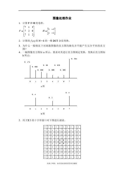
__________________________________________________图像处理作业1. 计算 F 和 H 的卷积。
7 1 3 F 7 2 07 1 2H1 11 12. 计算的 f (x) 的 N=8 的一维 DCT 余弦变换。
3. 为什么一般情况下对离散图像的直方图均衡化并不能产生完全平坦的直方 图?4. 一幅图像直方图如 a 所示,要求对其进行直方图规定变换,变换后直方图如b 所示:0.3840.1740.0880.080.0580.0860.0680.06201234567a图0.40.20.401234567b图5. 用 5 X 5 的十字形窗口对下图进行滤波。
1111111111 1 1 1 1 1 1 1 1 11 1115555111 1155555511 1155885511 1155885511 1155555511 1115555111 1111111111 1111111111收集于网络,如有侵权请联系管理员删除__________________________________________________6. 已知符号 a,e,i,o,u,? 的出现概率分别是 0.2 , 0.3, 0.1 ,0.2 ,0.1 ,0.1 , 对字符串 aieoau 进行算术编码;如果一个字符串(共四位)的算术编码是 0.23355,对其进行算术解码,求这字符串是什么。
7. 已知符号 a,e,i,o,u,? 的出现概率分别是 0.2 , 0.3, 0.1 ,0.2 ,0.1 ,0.1 , 求这些字符的霍夫曼编码,及编码后的平均码长。
收集于网络,如有侵权请联系管理员删除__________________________________________________答案: 7 6 2 31. F * H 14 11 0 314 11 1 2 761 22. F (0) 2 4 ( f0 f1 f 2 f3 f 4 f 5 f6 f7 )F (1)1 2[(f0f7)c os16(f1f6)cos3 16(f2f5)cos5 16(f3f4)cos7 16]F (2)1 2[(f0f3f4f7)cos 8 ( f1f2f5f6)cos3 8]F (3)1 2[( f0f3 7) cos 16(f67 f1) cos 16(f5f2)cos 16(f45 f3 ) cos 16 ]2 F (4) 4 ( f0 f1 f 2 f3 f 4 f 5 f6 f7 )F (5)1 2[(f0f7)cos5 16(f6f1)cos 16(f2f5)cos7 16(f3f4)cos3 16]F (2)1 2[(f0f3f4f7)cos3 8 ( f1f2f5 f6 ) cos 8 ]F (7)1 2[(f0f7)cos7 16(f6f1)cos5 16(f2f5)cos3 16(f4f3)cos 16]3.因为离散图像中灰度级是用离散的二进制整数表示的,所以均衡化的直方图 不能用连续的实数表示灰度,只能用近似的整数表示,这使得对离散图像的直方 图均衡化不能产生完全平坦的直方图。
数字图像处理每章课后题参考答案
数字图像处理每章课后题参考答案数字图像处理每章课后题参考答案第一章和第二章作业:1.简述数字图像处理的研究内容。
2.什么是图像工程?根据抽象程度和研究方法等的不同,图像工程可分为哪几个层次?每个层次包含哪些研究内容?3.列举并简述常用表色系。
1.简述数字图像处理的研究内容?答:数字图像处理的主要研究内容,根据其主要的处理流程与处理目标大致可以分为图像信息的描述、图像信息的处理、图像信息的分析、图像信息的编码以及图像信息的显示等几个方面,将这几个方面展开,具体有以下的研究方向:1.图像数字化,2.图像增强,3.图像几何变换,4.图像恢复,5.图像重建,6.图像隐藏,7.图像变换,8.图像编码,9.图像识别与理解。
2.什么是图像工程?根据抽象程度和研究方法等的不同,图像工程可分为哪几个层次?每个层次包含哪些研究内容?答:图像工程是一门系统地研究各种图像理论、技术和应用的新的交叉科学。
根据抽象程度、研究方法、操作对象和数据量等的不同,图像工程可分为三个层次:图像处理、图像分析、图像理解。
图像处理着重强调在图像之间进行的变换。
比较狭义的图像处理主要满足对图像进行各种加工以改善图像的视觉效果。
图像处理主要在图像的像素级上进行处理,处理的数据量非常大。
图像分析则主要是对图像中感兴趣的目标进行检测和测量,以获得它们的客观信息从而建立对图像的描述。
图像分析处于中层,分割和特征提取把原来以像素描述的图像转变成比较简洁的非图形式描述。
图像理解的重点是进一步研究图像中各目标的性质和它们之间的相互联系,并得出对图像内容含义的理解以及对原来客观场景的解释,从而指导和规划行为。
图像理解主要描述高层的操作,基本上根据较抽象地描述进行解析、判断、决策,其处理过程与方法与人类的思维推理有许多相似之处。
第三章图像基本概念1.图像量化时,如果量化级比较小时会出现什么现象?为什么?答:当实际场景中存在如天空、白色墙面、人脸等灰度变化比较平缓的区域时,采用比较低的量化级数,则这类图像会在画面上产生伪轮廓(即原始场景中不存在的轮廓)。
图像工程考试复习习题课
利用投影变换矩阵
c x
1 0
ch
Pwh
0 0
1 0
0 0
y
z T
lX l Z
0 0 1
1 l
0 kX kX
0
kY
kY
0 kZ kZ
1
k
kZ
l
k
lY lZ
lZ lZ
T
0.2
0.4
00),图像平面坐标(-0.2,-0.4)
第二章
(2) 2.0mm/14mm=6cm/u u=14*6/2(cm)=42cm
第二章
2-4 空间点(1,2,3)经l=0.5的镜头透视后的摄 像机坐标和图像平面坐标各是什么?
第二章
2-4 空间点(1,2,3)经l=0.5的镜头透视后的摄 像机坐标和图像平面坐标各是什么?
利用几何关系
x X X
q
8-通路长度4,m-通路长度6
3121
m-连接:同时存在4-连接和8-连 2 2 0 2
接时,优先采用4-连接
1211
p1 0 1 2
第三章
3-5 设给定如下平移变换矩阵T和尺度变换 矩阵S,分别计算对空间点(1,2,3)先平移变 换后尺度变换和先尺度变换后平移变换所 得到的结果,并进行比较讨论。
实际图像的尺寸是有限的,所以x和y的取值也是有限
的实数,f代表图像在点(x,y)的某种性质F的数值,其
取值也是有限的实数。
I (r,c)中(r,c)代表离散化后的(x,y),r表示图像的行,c
代表图像的列,I代表离散化后的f。I, r, c都是整数。
第一章
1-9 如果一个2×2模板的每个位置可表示 4种灰度,那么这个模板一共可表示多少 个灰度?
工程制图与识图阶段性作业及答案
工程制图与识图(高起专)阶段性作业1多选题1. 图样上的尺寸包括________ (5分)(A) 尺寸界线(B) 尺寸线(C) 尺寸起止符号(D) 尺寸数字参考答案:A,B,C,D2. 绘制工程图样有三种方法,分别是____________ (5分)(A) 徒手绘图(B) 尺规绘图(C) 计算机绘图(D) 素描参考答案:A,B,C3. 在绘图的过程中,可能会用到的工具有______________ (5分)(A) 丁字尺(B) 曲线板(C) 皮尺(D) 三棱尺参考答案:A,B,D4. 分规的作用是_______ (5分)(A) 绘制线段(B) 量取线段(C) 等分线段(D) 画圆和圆弧参考答案:B,C判断题5. 当直线或者平面平行于投影面时,其投影反映实长或实形,这体现了正投影法的实形性。
(5分)正确错误参考答案:正确解题思路:6. 正面投影与水平投影的长度相等,左右对正;正面投影与侧面投影的高度相等,上下平齐;水平投影与侧面投影宽度相等,前后对应。
即“长对正,高平齐,宽相等”。
(5分)正确错误参考答案:正确解题思路:7. 从下图中可以知道,直线AB平行于CD (5分)正确错误参考答案:正确解题思路:8. 由下图可以看出,直线AB和CD相互平行。
(5分)正确错误参考答案:错误解题思路:9. 已知A点坐标为(10, 15,8),B点坐标为(15,5,12 ),贝U A点在B点的上方。
(5分)正确错误参考答案:错误解题思路:10. 如下如所示,根据直线AB与投影面的相对位置可以看出AB为正平线。
(5分)正确错误参考答案:正确解题思路:11. 如图所示,判断直线AB和CD的重影点的可见性是否正确。
(5分)正确错误参考答案:正确解题思路:12. 如下图,可知直线AB CD的重影点的标识是错误的。
(5分)正确错误参考答案:错误解题思路:填空题13. 工程上常用的有—⑴—和⑵两类投影法。
(5分)(1).参考答案:中心投影法⑵.参考答案:平行投影法14. 平行投影法中,根据投影方向与投影面之间的几何关系,有⑶和⑷两种投影法,其中—(5)___ (投影法)在工程上应用最广。
(完整版)数字图像处理大作业
数字图像处理1.图像工程的三个层次是指哪三个层次?各个层次对应的输入、输出对象分别是什么?①图像处理特点:输入是图像,输出也是图像,即图像之间进行的变换。
②图像分割特点:输入是图像,输出是数据。
③图像识别特点:以客观世界为中心,借助知识、经验等来把握整个客观世界。
“输入是数据,输出是理解。
2.常用的颜色模型有哪些(列举三种以上)?并分别说明颜色模型各分量代表的意义。
①RGB(红、绿、蓝)模型②CMY(青、品红、黄)模型③HSI(色调、饱和度、亮度)模型3.什么是图像的采样?什么是图像的量化?1.采样采样的实质就是要用多少点来描述一幅图像,采样结果质量的高低就是用前面所说的图像分辨率来衡量。
简单来讲,对二维空间上连续的图像在水平和垂直方向上等间距地分割成矩形网状结构,所形成的微小方格称为像素点。
一副图像就被采样成有限个像素点构成的集合。
例如:一副640*480分辨率的图像,表示这幅图像是由640*480=307200个像素点组成。
2.量化量化是指要使用多大范围的数值来表示图像采样之后的每一个点。
量化的结果是图像能够容纳的颜色总数,它反映了采样的质量。
针对数字图像而言:采样决定了图像的空间分辨率,换句话说,空间分辨率是图像中可分辨的最小细节。
量化决定了图像的灰度级,即指在灰度级别中可分辨的最小变化。
数字图像处理(第三次课)调用图像格式转换函数实现彩色图像、灰度图像、二值图像、索引图像之间的转换。
图像的类型转换:对于索引图像进行滤波时,必须把它转换为RGB图像,否则对图像的下标进行滤波,得到的结果是毫无意义的;2.用MATLAB完成灰度图像直方图统计代码设计。
6789101112131415161718192021222324252627282930title('lady-lenna');if isrgb(a);b=rgb2gray(a);%RGB转换为灰度图像endsubplot(2,2,2);imshow(b);%显示图像title('ladygaga-lenna');[m,n]=size(a);%返回图像大小e=zeros(1,256);for k=0:255for i=1:mfor j=1:nif a(i,j)==ke(k+1)=e(k+1)+1;%灰度值相同的进行累加endendendendsubplot(2,2,4);bar(e);%画图像的灰度直方图title('灰度直方图');c=imrotate(a,20);%图像的旋转subplot(2,2,3);imshow(c);数字图像处理(第四次课)编写matlab函数,实现在医学图像中数字减影血管造影。
图像工程答案

1-9 如果一个2×2模板的每个位置可以表示4种灰度,那么这个模板一共可以表示多少个灰度?0~3->0~12答:13个灰度:0~12一共13个灰度1-12 试读出一个位图文件的文件头和位图信息部分,分析其中那些内容可以通过直接观察位图本身而得到?读取文件头和位图信息的matlab代码:info=imfinfo('lena.bmp'),x=imread('lena.bmp');Filename: 'C:\Documents and Settings\yisayu\桌面\lena.bmp'FileModDate: '04-Nov-2011 17:18:54'FileSize: 263222Format: 'bmp'FormatVersion: 'Version 3 (Microsoft Windows 3.x)'Width: 512Height: 512BitDepth: 8ColorType: 'indexed'FormatSignature: 'BM'NumColormapEntries: 256Colormap: [256x3 double]RedMask: []GreenMask: []BlueMask: []ImageDataOffset: 1078BitmapHeaderSize: 40NumPlanes: 1CompressionType: 'none'BitmapSize: 0HorzResolution: 3780VertResolution: 3780NumColorsUsed: 256NumImportantColors: 256答:这些信息可以直接观察位图得到:Width: 512 Height: 512 BitDepth: 81-14 找一个对应二值图像的TIFF文件,再找一个对应灰度图像的TIFF文件,看看他们的文件头有什么区别?二值图像的TIFF文件:TIFF File: 'C:\Documents and Settings\yisayu\桌面\img2.tif'Mode: 'r'Current Image Directory: 1Number Of Strips: 32SubFileType: Tiff.SubFileType.DefaultPhotometric: Tiff.Photometric.MinIsWhiteImageLength: 512ImageWidth: 512RowsPerStrip: 16BitsPerSample: 1Compression: ITTRLESampleFormat: Tiff.SampleFormat.UIntSamplesPerPixel: 1PlanarConfiguration: Tiff.PlanarConfiguration.ChunkyOrientation: Tiff.Orientation.TopLeft灰度图像的TIFF文件:TIFF File: 'C:\Documents and Settings\yisayu\桌面\img.tif'Mode: 'r'Current Image Directory: 1Number Of Strips: 32SubFileType: Tiff.SubFileType.DefaultPhotometric: Tiff.Photometric.MinIsBlackImageLength: 512ImageWidth: 512RowsPerStrip: 16BitsPerSample: 8Compression: pression.PackBitsSampleFormat: Tiff.SampleFormat.UIntSamplesPerPixel: 1PlanarConfiguration: Tiff.PlanarConfiguration.ChunkyOrientation: Tiff.Orientation.TopLeft所以观察得出结论:BitsPerStrip不同。
数字图像处理作业1
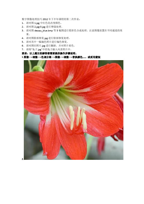
数字图像处理技巧2012年下半年课程的第二次作业:1、请对图1.jpg中红色花改变颜色。
2、请对图2.jpg-3.jpg进行增强处理。
3、请对图dessau_blue.bmp等5幅图进行假彩色合成处理,注意图像放置在不同通道的效果。
4、请对图脸部修复.jpg进行脸部修复处理。
5、请对其中一幅偏色照片进行偏色修复。
6、请对图旧照片.jpg进行翻新,并对照片着色。
7、请将”兔子.jpg”中的兔子融入风景照片中。
要求:以上题目的解答都需要提供操作步骤说明。
1.图像--->调整--->色调分离--->图像--->调整--->替换颜色。
或采用蒙版2.3.增强亮度色彩:图像--->调整--->对比度/亮度、色阶、曲线4.5.伪色彩增强:先观察其索引色模式,在该模式下,图层命令不可用。
执行图像-模式-颜色表,为不同灰度等级设置颜色,可观察伪彩色增强图像效果。
3.假色彩合成:打开三张图像--->图像--->模式--->灰度--->通道控制面板菜单中的合并通道--->对应选择--->完成合成--->4.放大--->工具箱中修复画笔工作--->alt选取--->修补--->缩小5.偏色修复:图像——>调整——>色彩平衡:6.旧照片翻新:先调整亮度对比度等,再放大,用仿制图章或污点修复工具对照片进行修改,之后在把人物抠出羽化边缘,用第一题的方法修改下颜色,再换上新背景,在用动作给图片加上相框:7.法一用魔棒进行抠图,把兔子抠出来调整边缘,再与原风景合并法二一用Photoshop打开原图,点击来到通道面板,选择黑白较为分明的红色通道,右击复制,得到红副本通道.二,再对副本通道执行CTRL+I反相三,用工具栏上的减淡工具对人物头发边缘进行减淡处理。
按住ctrl键同时点击红副本通道(载入选区)四,保持选区,返回图层面板,双击解锁背景图层五,给背景图层添加蒙版六,与原图合并,同理做另一只兔子7.总合并:将两只兔子拖入。
北航《工程图学》在线作业一
北航《工程图学》在线作业一
单选题多选题判断题
一、单选题(共 10 道试题,共 40 分。
)
1. 移出断面图的轮廓用()绘制,一般需画出剖面线
A. 粗实线
B. 细实线
C. 虚线
D. 点划线
-----------------选择:A
2. 纵向定位轴线的编写顺序为()
A. 从上至下
B. 从下至上
C. 从左至右
D. 从右至左
-----------------选择:B
3. ()基本体的特征是每个表面都是平面。
A. 平面
B. 圆柱
C. 圆锥
D. 斜面
-----------------选择:A
4. 物体上凡是与投影面倾斜的直线和平面,其投影成()的类似形。
A. 放大
B. 缩小
C. 同比例
D. 平行
-----------------选择:B
5. 组合体长宽高的每一个方向至少应有()主要尺寸基准
A. 一个
B. 两个
C. 三个
D. 四个
-----------------选择:A
6. 徒手画图的基本要求是()
A. 线条横平竖直
B. 尺寸准确
C. 快准好
D. 速度快
-----------------选择:A
7. 对表示外螺纹小径的细实线,一般按大径的()倍画出。
- 1、下载文档前请自行甄别文档内容的完整性,平台不提供额外的编辑、内容补充、找答案等附加服务。
- 2、"仅部分预览"的文档,不可在线预览部分如存在完整性等问题,可反馈申请退款(可完整预览的文档不适用该条件!)。
- 3、如文档侵犯您的权益,请联系客服反馈,我们会尽快为您处理(人工客服工作时间:9:00-18:30)。
图像工程作业1:梯度域图像融合(Gradient-Domain Fusion)O VERVIEWThis project explores gradient-domain processing, a simple technique with a broad set of applications including blending, tone-mapping, andnon-photorealistic rendering. For the core project, we will focus on "Poisson blending"; tone-mapping and NPR can be investigated as bells and whistles. The primary goal of this assignment is to seamlessly blend an object or texture from a source image into a target image. The simplest method would be to just copy and paste the pixels from one image directly into the other. Unfortunately, this will create very noticeable seams, even if the backgrounds arewell-matched. How can we get rid of these seams without doing too much perceptual damage to the source region?The insight is that people often care much more about the gradient of an image than the overall intensity. So we can set up the problem as finding values for the target pixels that maximally preserve the gradient of the source region without changing any of the background pixels. Note that we are making a deliberate decision here to ignore the overall intensity! So a green hat could turn red, but it will still look like a hat.We can formulate our objective as a least squares problem. Given the pixel intensities of the source image "s" and of the target image "t", we want to solve for new intensity values "v" within the source region "S":Here, each "i" is a pixel in the source region "S", and each "j" is a 4-neighbor of "i". Each summation guides the gradient values to match those of the source region. In the first summation, the gradient is over two variable pixels; in the second, one pixel is variable and one is in the fixed target region.The method presented above is called "Poisson blending". Check out the Perezet al. 2003 paper to see sample results, or to wallow in extraneous math. This is just one example of a more general set of gradient-domain processing techniques. The general idea is to create an image by solving for specified pixel intensities and gradients.A W ORDY E XPLANATION FROM YOUR TAAs an example, consider this picture of the bear and swimmers being pasted into a pool of water. Let's ignore the bear for a moment and consider the swimmers. In the above notation, the source image "s" is the original image the swimmers were cut out of; that image isn't even shown, because we are only interested in the cut-out of the swimmers, i.e., the region "S". "S" includes the swimmers and a bit of light blue background. You can clearly see the region "S" in the left image, as the cutout blends very poorly into the pool of water. The pool of water, before things were rudely pasted into it, is the target image "t".So, how do we blend in the swimmers? We construct a new image "v" whose gradients inside the region "S" are similar to the gradients of the cutout we're trying to paste in (swimmers + a little bit of background). The gradients won't end up matching exactly: the least squares solver will take any hard edges of the cutout at the boundary and smooth them by spreading the error over the gradients inside "S".Outside "S", "v" will match the pool. We won't even bother computing the gradients of the pool outside S; we'll just copy those pixels directly.In the first half of the large equation above, we set the gradients of "v" inside S. We loop over all the pixels inside the region S, and request that our new image "v" have the same gradients as the swimmers. The summation is over every pixel i in S; j is the 4 neighbors of i (left, right, up, and down, giving us both the x and y gradients. You may notice this equation counts all the gradients twice - is was simpler to write it this way. You actually don't have to double-count everything; it doesn't affect the result.) But what do we do around the boundary of "S"? I.e. what if i is inside S, but j is outside? That's the second half of the equation. (If you look closely at the variablesunder the summation sign, the S has a bar thing in front of it - that means the complement of S, or anything not in S. Thus, read "j in the 4-neighborhood of i, but j not in S"). In this case we aren't solving for a v_j, since j is not inside "S". So we just pluck the intensity value right out of the target image. Thus we use t_j. Remember, we aren't modifying t outside the area of S, so we know that v_j in this case isn't a variable: it's exactly equal to t_j.T OY P ROBLEM (20 PTS)The implementation for gradient domain processing isnot complicated, but it is easy to make a mistake, solet's start with a toy example. In this example we'llcompute the x and y gradients from an image s, thenuse all the gradients, plus one pixel intensity, toreconstruct an image v.Denote the intensity of the source image at (x, y) ass(x,y) and the values of the image to solve for as v(x,y).For each pixel, then, we have two objectives:add one more objective:correct, then you should recover the original image.Implementation DetailsThe first step is to write the objective function as a set of least squares constraints in the standard matrix form: (Av-b)^2. Here, "A" is a sparse matrix, "v" are the variables to be solved, and "b" is a known vector. It is helpful to keep a matrix "im2var" that maps each pixel to a variable number, such as:[imh, imw, nb] = size(im);im2var = zeros(imh, imw);im2var(1:imh*imw) = 1:imh*imw;(If you find that matlab trickery confusing, understand that you could have performed themapping between pixel and variable number manually each time: e.g. the pixel at s(r,c), uses the variable number (c-1)*imh+r. However, this trick will come in handy for Poisson blending, where the mapping is from an arbitrarily-shaped block of pixels and won't be such a simplefunction. So it makes sense to understand it now.)Then, you can write Objective 1 above as:e=e+1;A(e, im2var(y,x+1))=1;A(e, im2var(y,x))=-1;b(e) = s(y,x+1)-s(y,x);Here, "e" is used as an equation counter. Note that the y-coordinate is the first index in Matlab convention. Objective 2 is similar; add all the y-gradient constraints as more rows to the same matrices A and b. As another example, Objective 3 above can be written as:e=e+1;A(e, im2var(1,1))=1;b(e)=s(1,1);To solve for v, use v = A\b; or v = lscov(A, b); Then, copy each solved value to the appropriate pixel in the output image.P OISSON B LENDING (60 PTS)Step 1: Select source and target regions. Select the boundaries of a region in the source image and specify a location in the target image where it should be blended. Then, transform (e.g., translate) the source image so that indices of pixels in the source and target regions correspond. I've provided starter code (getMask.m, alignSource.m) to help with this. You may want to augment the code to allow rotation or resizing into the target region. You can be a bit sloppy about selecting the source region -- just make sure that the entire object is contained. Ideally, the background of the object in the source region and the surrounding area of the target region will be of similar color.Step 2: Solve the blending constraints:Step 3: Copy the solved values v_i into your target image. For RGB images, process each channel separately. Show at least three results of Poisson blending. Explain any failure cases (e.g., weird colors, blurred boundaries, etc.).Tips1. Pre-initialize your sparse matrix with sparse([], [], [], M, N, nzmax) for a matrix with M equations and N variables and at most nzmax non-zero entries.2. For your first blending example, try something that you know should work, such as the included penguins on top of the snow in the hiking image.3. Object region selection can be done very crudely, with lots of room aroundthe object.M IXED G RADIENTS (20 PTS)Follow the same steps as Poisson blending, but use the gradient in source or target with the larger magnitude as the guide, rather than the source gradient:Here "d_ij" is the value of the gradient from the source or the target image with larger magnitude, i.e. if abs(s_i-s_j) > abs(t_i-t_j), then d_ij = s_i-s_j; else d_ij = t_i-t_j. Show at least one result of blending using mixed gradients. Onepossibility is to blend a picture of writing on a plain background onto another image.B ELLS &W HISTLES (E XTRA P OINTS)Color2Gray (20 pts)Sometimes, in converting a color image to grayscale (e.g., when printing to a laser printer), we lose the important contrast information, making the image difficult to understand. For example, compare the color version of the image onright with its grayscale version produced byrgb2gray.Can you do better than rgb2gray?Gradient-domain processing provides oneavenue: create a gray image that has similarintensity to the rgb2gray output but has similar contrast to the original RGBimage. This is an example of a tone-mapping problem, conceptually similar to that of converting HDR images to RGB displays. To get credit for this, show the grayscale image that you produce (the numbers should be easily readable).Hint: Try converting the image to HSV space and looking at the gradients in each channel. Then, approach it as a mixed gradients problem where you also want to preserve the grayscale intensity.More gradient domain processing (up to 20 pts)Many other applications are possible, including non-photorealistic rendering, edge enhancement, and texture or color transfer. See Perez et al. 2003 orGradient Shop for further ideas.M ATERIALSImages, including the toy image, sample images for blending, and the color2gray image.∙Starter Code, including a top-level script and functions to select the source region and align source and target images for blending.D ELIVERABLESUse both words and images to show us what you've done.Place all code in your code/ directory. Include a README describing thecontents of each file.In the website in your www/ directory, please:∙Include a brief description of the project.∙Show your favorite blending result. Include: 1) the source and target image; 2) the blended image with the source pixels directly copied into the target region; 3) the final blend result. Briefly explain how it works, along with anything special that you did or tried. This should be with your own images, not the included samples. ∙Next, show at least two more results for Poisson blending, including one that doesn't work so well (failure example). Explain any difficulties and possiblereasons for bad results.∙Show at least one result for blending with mixed gradients. Again, show the source image, target image, and final result.Special thanks to Prof. Derek Hoiem who allowed me to copy this project from his Computational Photography course.要求:1.独立完成作业,不得拷贝或抄袭,否则以课程成绩不及格处理。