10金德环投资学第十章
投资学第10章

已知销售量、单位产品变动成本、固定成本总额,可以求得保本的单位价格。
盈亏平衡时单位价格= 变动成本总额+固定成本总额 销售量
可以求得盈亏平衡时的生产能力利用率指标:
盈亏平衡时生产能力利用率= 保本量 设计年产量
06:59:08
精品文档
练习题1:某企业固定费用为20000万,单 位变动费用为3000元,单价(dānjià)为5000 元。 求在上述条件下盈亏平衡点。
(5)绘制敏感性分析图。在敏感性分析图中,与横坐标相 交角度最大的曲线对应的因素(yīn sù)就是最敏感的因素 (yīn sù)。
(6)分析评价。从敏感性分析表和敏感性分析图可以 看出(kàn chū),净现值指标对年收入的变化最敏感。
06:59:08
精品文档
敏感性分析(fēnxī)的局限性
局限性
06:59:08
精品文档
10.2.2 敏感性分析
10.2 项目(xiàngmù)投资的不确定性分析
敏感性分析,是在诸多的不确定因素中,确定哪些是敏感 性因素,哪些是不敏感性因素,并分析敏感性因素对经济 效益的影响程度。
敏感性分析是动态分析方法,它引入了资金时间价值 的概念。它的主要分析是在现值的基础上进行的,计 算在不确定因素变化的情况下,项目的净现值和内部 收益率等经济效益指标会发生什么变化。
• ①求盈亏平衡产量Q?
• ②若2004年生产1200台,求:利润=? • •解③:若上级要求完成利润额5万元,则应完成产量?
Cv=100000/1000=100 Q=80000/(200-100)=800台
Z=(P-Cv)*Q- Cf =(200-100)*1200-80000=4万 Q=(Z+ Cf)/(P-Cv)=(50000+80000)/(200-100)=1300台
金德环《投资学》课后习题答案
金德环《投资学》课后习题答案习题答案第一章习题答案第二章习题答案练习题1:答案:(1),公司股票的预期收益率与标准差为:Er,,,,,,,0.570.350.2206,,,,,,,,A1/2222,, ,0.5760.3560.22068.72,,,,,,,,,,,,,,A,,(2),公司和,公司股票的收益之间的协方差为:Covrr,0.5762510.50.3561010.5,,,,,,,,,,,,,,,,,AB ,,,,,,0.22062510.590.5,,,,(3),公司和,公司股票的收益之间的相关系数为:Covrr,,,,90.5AB ,,,,,0.55AB,8.7218.90,,AB练习题2:答案:如果,,,的投资投资于,公司,余下,,,投资于,公司的股票,这样得出的资产组合的概率分布如下:钢生产正常年份钢生产异常年份股市为牛市股市为熊市概率 0.5 0.3 0.2 资产组合收益率(,) ,, ,., -2.5 得出资产组合均值和标准差为:Er=0.516+0.32.5+0.2-2.5=8.25,,,,,,,,,,组合1/22222,, ,=0.516-8.25+0.32.5-8.25+0.2-2.5-8.25+0.2-2.5-8.25=7.94,,,,,,,,组合,,1/22222,=0.518.9+0.58.72+20.50.5-90.5=7.94,,,,,,,,,,,,,,,组合,,练习题3:答案:尽管黄金投资独立看来似有股市控制,黄金仍然可以在一个分散化的资产组合中起作用。
因为黄金与股市收益的相关性很小,股票投资者可以通过将其部分资金投资于黄金来分散其资产组合的风险。
练习题4:答案:通过计算两个项目的变异系数来进行比较:0.075 CV==1.88A0.040.09 CV==0.9B0.1考虑到相对离散程度,投资项目B更有利。
练习题5:答案:R(1)回归方程解释能力到底如何的一种测度方法式看的总方差中可被方程解释的方差所it2,占的比例。
(本科)投资学NO10教学课件

第二节 行 业 分 析
行业是指一群提供类似产品或服务的企业团体。 随着时间的演变,行业的增长率和盈利水平往往 经历明显的变化。
第二节 行 业 分 析
一个典型的行业生命周期分为四个阶段:创业阶 段,具有较高的发展速度;成长阶段,发展速度 降低,但是仍然高于经济整体速度;成熟阶段, 发展速度与整体经济一致;衰退阶段,发展速度 低于经济中的其他行业,或者已经慢慢萎缩。
第一节 宏观经济分析
利率升高鼓励公司和个人少消费、多储蓄。高利率 降低未来现金流现值,所以会降低投资机会的吸引 力。因此,实际利率是企业投资成本的关键决定因 素。人们对住房等高价耐用消费品通常通过融资得 到满足,由于利率会影响利息支付,因而它们对利 率高度敏感。
第一节 宏观经济分析
5.汇率
汇率是指按照购买力平价测度的两国货币的比率关 系。汇率的变动直接影响着本国产品在国际市场的 竞争能力,从而对本国经济增长造成一定影响。本 币对外币贬值利好出口导向型经济。
第一节 宏观经济分析
3.失业率
失业率是指正在寻找工作的劳动力占总劳动力的百 分比。失业率度量了经济运行中生产能力极限的运 用程度。失业率只与劳动力有关,但是从失业率中 可以得到其他生产要素的信息,从而进一步了解经 济运行状况。
第一节 宏观经济分析
4.利率
利率是由可贷资金的供求关系决定的。当利率降低 时,可贷资金的需求量增加。利率降低增加了对厂 房、设备和存货等资产投资的盈利性,降低了住房 抵押贷款的成本,增加了对借入资金的需求量。当 利率上升时,情况相反。
引导案例
(3) 汇率基本稳定、货币持续紧缩难认可。目前的人民币 汇率已经较为稳定,降低汇率波动则可以稳定市场预期、减 少流动性冲击,对国内股票和债券市场形成利好。年初以来 央行的操作结束了宽松已经被公认,但是进入紧缩则很难被 认可。
复旦大学经济学院硕士研究生入学考试参考书目

复旦大学经济学院硕士研究生入学考试参考书目复旦大学经济学院硕士研究生入学考试参考书目0 1政治经济学:①《政治经济学教材》蒋学模主编上海人民出版社②《西方经济学》袁志刚高等教育出版社③《微观经济学》陈钊、陆铭高等教育出版社 2月④《宏观经济学》袁志刚、樊潇彦高等教育出版社 2月⑤《现代西方经济学习题指南》尹伯成复旦大学出版社⑥《国际经济学》华民复旦大学出版社0 2经济思想史:同0 1专业0 3经济史:同0 1专业0 4西方经济学:同0 1专业0 5世界经济:同0 1专业0 0发展经济学:同0 1专业0 1欧盟经济:同0 1专业020201国民经济学:同0 1专业020202区域经济学:同0 1专业020203财政学:同0 1专业020204金融学:①至⑤同0 1专业①至⑤⑥《国际金融新编》(第四版)姜波克复旦大学出版社⑦《现代货币银行学教程》(第三版)胡庆康复旦大学出版社⑧《投资学》(第二版)刘红忠高等教育出版社020206国际贸易学:同0 1专业020207劳动经济学:同0 1专业020209数量经济学:同0 1专业020221产业组织学:同0 1专业025100(专业学位)金融硕士:待教育部考试大纲公布后,再确定参考书目。
812金融学基础参考书目和考试大纲金融学基础分经济学(微观经济学与宏观经济学)、宏观金融(国际金融与货币银行学)、微观金融(投资学与公司金融)三部分,各部分各占比1/3。
参考书目为:1、《微观经济学:现代观点(第七版)》范里安,格致出版社,2、《宏观经济学》曼昆(Mankiw),中国人民大学出版社,3、《国际金融学》奚君羊,上海财经大学出版社,4、《货币银行学》(第二版)戴国强,高等教育出版社,5、《投资学》金德环,高等教育出版社,6、《公司理财》(原书第7版)斯蒂芬. 罗斯等,机械工业出版,考试大纲为:微观经济学部分:一、消费者行为:预算约束、消费者偏好与效用函数、消费者最优选择、需求、斯勒茨基方程、消费者剩余二、不确定性:期望(预期)效用函数、风险规避、风险性资产三、生产者行为:技术、成本最小化、成本曲线、利润最大化、企业供给四、竞争性市场:市场需求、行业供给、短期均衡、长期均衡、经济租金、竞争性市场中的税收与税负转嫁五、不完全竞争市场:垄断定价、价格歧视、自然垄断、寡头产量竞争、产量合谋、产量领导者模型、价格领导者模型六、博弈论基础:支付矩阵、纳什均衡、混合策略纳什均衡七、一般均衡:交换经济均衡、帕累托有效、均衡与效率(福利经济学第一定理和福利经济学第二定理)八、外部性与公共品宏观经济学部分:一、国民收入核算与国民收入恒等式二、IS-LM模型1、收入与支出2、IS-LM模型3、IS-LM模型中的财政、货币政策4、开放经济下IS-LM模型政策效应分析三、总供给与总需求1、总供给与总需求2、失业与通货膨胀四、经济增长1、新古典经济增长模型2、内生经济增长模型五、消费1、持久性收入消费理论2、不确定条件下的消费行为六、投资1、基本投资理论2、投资的Q理论七、经济周期1、价格错觉模型2、实际经济周期模型3、粘性价格模型八、宏观经济政策争论1、积极与消极政策2、政策时滞与政策效应3、规则与相机抉择国际金融部分:一、国际收支及宏观经济均衡1、国际收支的概念、国际收支平衡表的内容、各种国际收支理论2、国际收支分析方法、国际收支性质上的不平衡及其成因、国际收支的自动调节机制3、国际收支的弹性论、吸收论、乘数论和货币论4、国际收支失衡的政策调节方法及其效能5、开放经济条件下的内部与外部均衡、米德冲突、丁伯根法则和政策分配原则、斯旺模型和蒙代尔模型6、中国的国际收支二、外汇、汇率及汇率制度1、外汇的概念及货币的可兑换性、汇率的标价方法及货币的升值与贬值、汇率种类、外汇风险、外汇市场的概念、主要的外汇交易2、汇率的决定基础、各种汇率决定理论、各种外汇交易和外汇风险防范方法3、影响汇率变动的主要因素、汇率变动对经济的影响、购买力平价论、利率平价论、货币论(灵活价格货币模型和粘性价格货币模型)、资产组合论4、固定汇率、浮动汇率及中间汇率制度5、最优货币区理论、蒙代尔-弗莱明模型、三元难题、外汇干预6、中国的汇率制度三、国际储备和国际货币体系1、国际储备的内涵、国际清偿力、国际储备的规模与结构管理2、多种货币储备体系的成因和特点3、国际金本位制度和储备货币本位制度的运作机制、布雷顿森林体系的建立及其崩溃、买加体系的成因、欧元区的形成和发展4、中国的国际储备管理和人民币国际化四、国际金融市场、国际资本流动和货币危机1、国际金融市场的概念、构成、发展过程2、国际资本市场的涵义和优势3、国际货币市场以及欧洲货币市场的特点、经营活动、优劣及其影响4、国际资本流动的主要类型和动因、国际中长期资本流动和国际短期资本流动的形式和特点5、货币危机的基本概念及其成因、三代货币危机模型的基本机理和经济影响货币银行部分:一、货币、信用与利息1、货币与货币制度:货币的起源和发展、货币的职能、货币制度、货币的层次2、信用:信用的产生与发展、现代信用的基本形式、各种主要的信用工具、信用的作用3、利息与利率:利息本质的理论、利率的种类、利率的作用、利率的决定、利率的结构二、金融市场1、直接融资与间接融资、金融市场的功能、金融市场的分类、金融创新2、货币市场:特征、主要工具3、资本市场:特征、主要工具4、其它金融市场与工具:金融衍生产品及市场、外汇市场、黄金市场三、金融机构体系1、商业银行:产生与发展、主要业务、经营管理、巴塞尔协议2、投资银行:产生与发展、主要业务、分业经营与混业经营3、其它金融机构:存款型、契约型、投资型、政策型4、中央银行:产生与发展、主要业务、性质与地位、职能与作用5、金融危机与金融监管:金融危机的原因与表现、金融监管的必要性与主要措施四、货币理论与政策1、货币供给:商业银行存款创造、基础货币、货币乘数、乔顿模型、内生性与外生性2、货币需求:影响货币需求的因素、传统货币数量说、流动性偏好理论及其发展、现代货币数量说3、货币政策:货币政策工具、货币政策中间目标、货币政策最终目标、菲利普斯曲线、单一规则与相机抉择、货币政策的传导机制4、通货膨胀与通货紧缩:通货膨胀的度量、成因与治理、通货紧缩5、金融与经济发展:金融抑制、金融发展投资学部分:一、证券市场和证券投资的收益与风险1、基本概念、证券市场的要素及运行(1)证券、投资、金融市场、各类金融工具的概念、特点与分类(2)证券市场主体、证券市场中介(3)证券发行与交易的方式和运行规则2、证券投资收益和风险(1)证券投资收益和风险的种类(2)各种收益率的计算(3)投资风险的衡量二、证券投资组合管理1、多样化与组合构成(1)有效集及无差异曲线(2)最佳资产组合的选择和投资分散化2、有效市场与资本资产定价模型(1)有效市场理论(2)资本资产定价模型3、因素模型与套利定价理论(1)因素模型(2)套利定价理论4、资产配置三、投资工具分析和投资业绩评估1、股票、债券和证券投资基金(1)股票定价模型与股票投资分析(2)债券定价分析与债券组合管理(3)证券投资基金的运作与管理2、期权和期货(1)期权和期货的原理、功能及品种(2)期权定价模型与期货价格决定(3)期权和期货的交易机制、交易策略3、投资绩效评估公司金融部分:一、公司概论与资本预算1、公司概论:公司制企业、公司治理、公司目标、净营运资本、财务现金流量。
投资学第十章PPT课件
• rf= 3% 和RP= 7 . 5%
精选课件
7
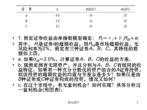
• 4. 假定F1与F2为两个独立的经济因素。无 风险利率为6%,并且,所有的股票都有独 立的企业特有(风险)因素,其标准差为4 5%。 下面是优化的资产组合,在这个经济体系 中,试进行期望收益-贝塔的相关性分析。
• c. The CAPM assumes that one specific factor explains security returns but APT does not.
• State whether each of the consultant’s arguments is correct or incorrect. Indicate, for each incorrect argument, why the argument is incorrect.
• a. 确定期望收益(以美元计)。其收益的标准差 为多少?
• b. 如果分析家验证了50种股票而不是20种,那 么答案又如何?100种呢?
精选课件
15
• a等量地卖空10种负α的股票并将收入等量投资 于10种正的股票,将消除市场的风险暴露并构 建一个零投资的资产组合。预期的美元收益为: 1 000 000 ×0.02+(-1 000 000)(-0.02)= 40 000美元。该资产组合的β为零,因为是等权重 的,其中一半的权数为负,所有的β都等于1。 因此,整体风险中系统性的成分为0。但是, 分析家的利润的方差却不为零,因为这一资产 组合没有充分分散化。总体方差就等于非系统 风险σ2= σ2 (ep) = σ2(ei)/n= 302/20 = 45且σ = 6.7 1%
投资经济学(第9-10章)

03
CATALOGUE
投资工具与投资策略
股票投资策略
01
02
03
成长投资策略
关注高成长潜力公司,寻 求长期资本增值。
价值投资策略
寻找被低估的公司股票, 期待市场对其重新评估。
技术分析策略
利用图表、指标等工具分 析股票价格波动,预测未 来走势。
债券投资策略
利率预期策略
基于对未来利率走势的预测,选择相应久期 和票息的债券。
提高投资者权益保护水平
完善法律法规
强化监管措施
建立健全投资者权益保护的法律法规体系 ,明确投资者的权利和义务,加大对违法 行为的惩处力度。
加强对金融机构和上市公司的监管力度, 确保其合规经营和充分披露信息,保障投 资者的合法权益。
推动投资者参与公司治理
加强国际合作与交流
鼓励投资者积极参与上市公司的治理活动 ,如股东大会、董事会等,促进公司规范 运作和提升治理水平。
算法交易
人工智能通过算法交易,实现交易的自动化和智能化,提高交易效率和收益。
区块链技术对投资领域的影响
01
去中心化投资
区块链技术的去中心化特点,使 得投资者能够直接参与项目投资 ,降低了中介成本和风险。
02
数字资产投资
区块链技术催生了数字资产市场 ,投资者可以通过投资数字资产 获取收益。
03
智能合约与自动化 执行
投资经济学(第9-10章)
汇报人:XX
CATALOGUE
目 录
• 第9章 资本市场与投资 • 第10章 投资决策与风险管理 • 投资工具与投资策略 • 投资绩效评估与投资者保护 • 未来投资趋势与展望
01
CATALOGUE
第9章 资本市场与投资
投资学第10版课后习题答案
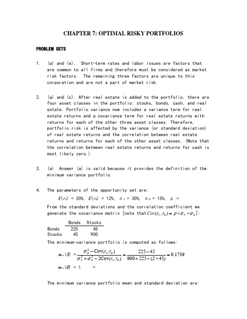
CHAPTER 7: OPTIMAL RISKY PORTFOLIOSPROBLEM SETS1. (a) and (e). Short-term rates and labor issues are factors thatare common to all firms and therefore must be considered as market risk factors. The remaining three factors are unique to this corporation and are not a part of market risk.2. (a) and (c). After real estate is added to the portfolio, there arefour asset classes in the portfolio: stocks, bonds, cash, and real estate. Portfolio variance now includes a variance term for real estate returns and a covariance term for real estate returns with returns for each of the other three asset classes. Therefore,portfolio risk is affected by the variance (or standard deviation) of real estate returns and the correlation between real estatereturns and returns for each of the other asset classes. (Note that the correlation between real estate returns and returns for cash is most likely zero.)3. (a) Answer (a) is valid because it provides the definition of theminimum variance portfolio.4. The parameters of the opportunity set are:E (r S ) = 20%, E (r B ) = 12%, σS = 30%, σB = 15%, ρ =From the standard deviations and the correlation coefficient we generate the covariance matrix [note that (,)S B S B Cov r r ρσσ=⨯⨯]: Bonds Stocks Bonds 225 45 Stocks 45 900The minimum-variance portfolio is computed as follows:w Min (S ) =1739.0)452(22590045225)(Cov 2)(Cov 222=⨯-+-=-+-B S B S B S B ,r r ,r r σσσ w Min (B ) = 1 =The minimum variance portfolio mean and standard deviation are:E (r Min ) = × .20) + × .12) = .1339 = %σMin = 2/12222)],(Cov 2[B S B S B B S Sr r w w w w ++σσ = [ 900) + 225) + (2 45)]1/2= %5.Proportion in Stock Fund Proportionin Bond Fund ExpectedReturnStandard Deviation% % % %minimumtangencyGraph shown below.0.005.0010.0015.0020.0025.000.00 5.00 10.00 15.00 20.00 25.00 30.00Tangency PortfolioMinimum Variance PortfolioEfficient frontier of risky assetsCMLINVESTMENT OPPORTUNITY SETr f = 8.006. The above graph indicates that the optimal portfolio is thetangency portfolio with expected return approximately % andstandard deviation approximately %.7. The proportion of the optimal risky portfolio invested in the stockfund is given by:222[()][()](,)[()][()][()()](,)S f B B f S B S S f B B f SS f B f S B E r r E r r Cov r r w E r r E r r E r r E r r Cov r r σσσ-⨯--⨯=-⨯+-⨯--+-⨯[(.20.08)225][(.12.08)45]0.4516[(.20.08)225][(.12.08)900][(.20.08.12.08)45]-⨯--⨯==-⨯+-⨯--+-⨯10.45160.5484B w =-=The mean and standard deviation of the optimal risky portfolio are:E (r P ) = × .20) + × .12) = .1561 = % σp = [ 900) +225) + (2× 45)]1/2= %8. The reward-to-volatility ratio of the optimal CAL is:().1561.080.4601.1654p fpE r r σ--==9. a. If you require that your portfolio yield an expected return of14%, then you can find the corresponding standard deviation from the optimal CAL. The equation for this CAL is:()().080.4601p fC f C C PE r r E r r σσσ-=+=+If E (r C ) is equal to 14%, then the standard deviation of the portfolio is %.b. To find the proportion invested in the T-bill fund, rememberthat the mean of the complete portfolio ., 14%) is an average of the T-bill rate and the optimal combination of stocks and bonds (P ). Let y be the proportion invested in the portfolio P . The mean of any portfolio along the optimal CAL is:()(1)()[()].08(.1561.08)C f P f P f E r y r y E r r y E r r y =-⨯+⨯=+⨯-=+⨯-Setting E (r C ) = 14% we find: y = and (1 − y ) = (the proportion invested in the T-bill fund).To find the proportions invested in each of the funds, multiply times the respective proportions of stocks and bonds in the optimal risky portfolio:Proportion of stocks in complete portfolio = =Proportion of bonds in complete portfolio = =10. Using only the stock and bond funds to achieve a portfolio expectedreturn of 14%, we must find the appropriate proportion in the stock fund (w S) and the appropriate proportion in the bond fund (w B = 1 −w S) as follows:= × w S + × (1 −w S) = + × w S w S =So the proportions are 25% invested in the stock fund and 75% inthe bond fund. The standard deviation of this portfolio will be:σP = [ 900) + 225) + (2 45)]1/2 = %This is considerably greater than the standard deviation of %achieved using T-bills and the optimal portfolio.11. a.Even though it seems that gold is dominated by stocks, gold mightstill be an attractive asset to hold as a part of a portfolio. Ifthe correlation between gold and stocks is sufficiently low, goldwill be held as a component in a portfolio, specifically, theoptimal tangency portfolio.b.If the correlation between gold and stocks equals +1, then no onewould hold gold. The optimal CAL would be composed of bills andstocks only. Since the set of risk/return combinations of stocksand gold would plot as a straight line with a negative slope (seethe following graph), these combinations would be dominated bythe stock portfolio. Of course, this situation could not persist.If no one desired gold, its price would fall and its expectedrate of return would increase until it became sufficientlyattractive to include in a portfolio.12. Since Stock A and Stock B are perfectly negatively correlated, arisk-free portfolio can be created and the rate of return for thisportfolio, in equilibrium, will be the risk-free rate. To find theproportions of this portfolio [with the proportion w A invested inStock A and w B = (1 –w A) invested in Stock B], set the standarddeviation equal to zero. With perfect negative correlation, theportfolio standard deviation is:σP = Absolute value [w AσA w BσB]0 = 5 × w A− [10 (1 –w A)] w A =The expected rate of return for this risk-free portfolio is:E(r) = × 10) + × 15) = %Therefore, the risk-free rate is: %13. False. If the borrowing and lending rates are not identical, then,depending on the tastes of the individuals (that is, the shape oftheir indifference curves), borrowers and lenders could havedifferent optimal risky portfolios.14. False. The portfolio standard deviation equals the weighted averageof the component-asset standard deviations only in the special case that all assets are perfectly positively correlated. Otherwise, as the formula for portfolio standard deviation shows, the portfoliostandard deviation is less than the weighted average of thecomponent-asset standard deviations. The portfolio variance is aweighted sum of the elements in the covariance matrix, with theproducts of the portfolio proportions as weights.15. The probability distribution is:Probability Rate ofReturn100%−50Mean = [ × 100%] + [ × (-50%)] = 55%Variance = [ × (100 − 55)2] + [ × (-50 − 55)2] = 4725Standard deviation = 47251/2 = %16. σP = 30 = y× σ = 40 × y y =E(r P) = 12 + (30 − 12) = %17. The correct choice is (c). Intuitively, we note that since allstocks have the same expected rate of return and standard deviation, we choose the stock that will result in lowest risk. This is thestock that has the lowest correlation with Stock A.More formally, we note that when all stocks have the same expected rate of return, the optimal portfolio for any risk-averse investor is the global minimum variance portfolio (G). When the portfolio is restricted to Stock A and one additional stock, the objective is to find G for any pair that includes Stock A, and then select thecombination with the lowest variance. With two stocks, I and J, theformula for the weights in G is:)(1)(),(Cov 2),(Cov )(222I w J w r r r r I w Min Min J I J I J I J Min -=-+-=σσσSince all standard deviations are equal to 20%:(,)400and ()()0.5I J I J Min Min Cov r r w I w J ρσσρ====This intuitive result is an implication of a property of any efficient frontier, namely, that the covariances of the global minimum variance portfolio with all other assets on the frontier are identical and equal to its own variance. (Otherwise, additional diversification would further reduce the variance.) In this case, the standard deviation of G(I, J) reduces to:1/2()[200(1)]Min IJ G σρ=⨯+This leads to the intuitive result that the desired addition would be the stock with the lowest correlation with Stock A, which is Stock D. The optimal portfolio is equally invested in Stock A and Stock D, and the standard deviation is %.18. No, the answer to Problem 17 would not change, at least as long asinvestors are not risk lovers. Risk neutral investors would not care which portfolio they held since all portfolios have an expected return of 8%.19. Yes, the answers to Problems 17 and 18 would change. The efficientfrontier of risky assets is horizontal at 8%, so the optimal CAL runs from the risk-free rate through G. This implies risk-averse investors will just hold Treasury bills.20. Rearrange the table (converting rows to columns) and compute serialcorrelation results in the following table:Nominal RatesFor example: to compute serial correlation in decade nominalreturns for large-company stocks, we set up the following twocolumns in an Excel spreadsheet. Then, use the Excel function“CORREL” to calculate the correlation for the data.Decade Previous1930s%%1940s%%1950s%%1960s%%1970s%%1980s%%1990s%%Note that each correlation is based on only seven observations, so we cannot arrive at any statistically significant conclusions.Looking at the results, however, it appears that, with theexception of large-company stocks, there is persistent serialcorrelation. (This conclusion changes when we turn to real rates in the next problem.)21. The table for real rates (using the approximation of subtracting adecade’s average inflation from the decade’s average nominalreturn) is:Real RatesSmall Company StocksLarge Company StocksLong-TermGovernmentBondsIntermed-TermGovernmentBondsTreasuryBills 1920s1930s1940s1950s1960s1970s1980s1990sSerialCorrelationWhile the serial correlation in decade nominal returns seems to be positive, it appears that real rates are serially uncorrelated. The decade time series (although again too short for any definitiveconclusions) suggest that real rates of return are independent from decade to decade.22. The 3-year risk premium for the S&P portfolio is, the 3-year risk premium for thehedge fund portfolio is S&P 3-year standard deviation is 0. The hedge fund 3-year standard deviation is 0. S&P Sharpe ratio is = , and the hedge fund Sharpe ratio is = .23. With a ρ = 0, the optimal asset allocation is,.With these weights,EThe resulting Sharpe ratio is = . Greta has a risk aversion of A=3, Therefore, she will investyof her wealth in this risky portfolio. The resulting investment composition will be S&P: = % and Hedge: = %. The remaining 26% will be invested in the risk-free asset.24. With ρ = , the annual covariance is .25. S&P 3-year standard deviation is . The hedge fund 3-year standard deviation is . Therefore, the 3-year covariance is 0.26. With a ρ=.3, the optimal asset allocation is, .With these weights,E. The resulting Sharpe ratio is = . Notice that the higher covariance results in a poorer Sharpe ratio.Greta will investyof her wealth in this risky portfolio. The resulting investment composition will be S&P: =% and hedge: = %. The remaining % will be invested in the risk-free asset.CFA PROBLEMS1. a. Restricting the portfolio to 20 stocks, rather than 40 to 50stocks, will increase the risk of the portfolio, but it ispossible that the increase in risk will be minimal. Suppose that, for instance, the 50 stocks in a universe have the same standard deviation () and the correlations between each pair areidentical, with correlation coefficient ρ. Then, the covariance between each pair of stocks would be ρσ2, and the variance of an equally weighted portfolio would be:222ρσ1σ1σnn n P -+=The effect of the reduction in n on the second term on theright-hand side would be relatively small (since 49/50 is close to 19/20 and ρσ2 is smaller than σ2), but thedenominator of the first term would be 20 instead of 50. For example, if σ = 45% and ρ = , then the standard deviation with 50 stocks would be %, and would rise to % when only 20 stocks are held. Such an increase might be acceptable if the expected return is increased sufficiently.b. Hennessy could contain the increase in risk by making sure thathe maintains reasonable diversification among the 20 stocks that remain in his portfolio. This entails maintaining a low correlation among the remaining stocks. For example, in part (a), with ρ = , the increase in portfolio risk was minimal. As a practical matter, this means that Hennessy would have to spread his portfolio among many industries; concentrating on just a few industries would result in higher correlations among the included stocks.2. Risk reduction benefits from diversification are not a linearfunction of the number of issues in the portfolio. Rather, the incremental benefits from additional diversification are mostimportant when you are least diversified. Restricting Hennessy to 10 instead of 20 issues would increase the risk of his portfolio by a greater amount than would a reduction in the size of theportfolio from 30 to 20 stocks. In our example, restricting the number of stocks to 10 will increase the standard deviation to %. The % increase in standard deviation resulting from giving up 10 of20 stocks is greater than the % increase that results from givingup 30 of 50 stocks.3. The point is well taken because the committee should be concernedwith the volatility of the entire portfolio. Since Hennessy’sportfolio is only one of six well-diversified portfolios and issmaller than the average, the concentration in fewer issues mighthave a minimal effect on the diversification of the total fund.Hence, unleashing Hennessy to do stock picking may be advantageous.4. d. Portfolio Y cannot be efficient because it is dominated byanother portfolio. For example, Portfolio X has both higherexpected return and lower standard deviation.5. c.6. d.7. b.8. a.9. c.10. Since we do not have any information about expected returns, wefocus exclusively on reducing variability. Stocks A and C have equal standard deviations, but the correlation of Stock B with Stock C is less than that of Stock A with Stock B . Therefore, a portfoliocomposed of Stocks B and C will have lower total risk than aportfolio composed of Stocks A and B.11. Fund D represents the single best addition to complementStephenson's current portfolio, given his selection criteria. Fund D’s expected return percent) has the potential to increase theportfolio’s return somewhat. Fund D’s relatively low correlation with his current portfolio (+ indicates that Fund D will providegreater diversification benefits than any of the other alternativesexcept Fund B. The result of adding Fund D should be a portfolio with approximately the same expected return and somewhat lower volatility compared to the original portfolio.The other three funds have shortcomings in terms of expected return enhancement or volatility reduction through diversification. Fund A offers the potential for increasing the portfolio’s return but is too highly correlated to provide substantial volatility reduction benefits through diversification. Fund B provides substantial volatility reduction through diversification benefits but is expected to generate a return well below the current portfolio’s return. Fund C has the greatest potential to increase the portfolio’s return but is too highly correlated with the current portfolio to provide substantial volatility reduction benefits through diversification.12. a. Subscript OP refers to the original portfolio, ABC to thenew stock, and NP to the new portfolio.i. E(r NP) = w OP E(r OP) + w ABC E(r ABC) = + = %ii. Cov = ρOP ABC = =iii. NP = [w OP2OP2 + w ABC2ABC2 + 2 w OP w ABC(Cov OP , ABC)]1/2= [ 2 + + (2 ]1/2= % %b. Subscript OP refers to the original portfolio, GS to governmentsecurities, and NP to the new portfolio.i. E(r NP) = w OP E(r OP) + w GS E(r GS) = + = %ii. Cov = ρOP GS = 0 0 = 0iii. NP = [w OP2OP2 + w GS2GS2 + 2 w OP w GS (Cov OP , GS)]1/2= [ + 0) + (2 0)]1/2= % %c. Adding the risk-free government securities would result in alower beta for the new portfolio. The new portfolio beta will bea weighted average of the individual security betas in theportfolio; the presence of the risk-free securities would lowerthat weighted average.d. The comment is not correct. Although the respective standarddeviations and expected returns for the two securities underconsideration are equal, the covariances between each security andthe original portfolio are unknown, making it impossible to drawthe conclusion stated. For instance, if the covariances aredifferent, selecting one security over the other may result in alower standard deviation for the portfolio as a whole. In such acase, that security would be the preferred investment, assumingall other factors are equal.e. i. Grace clearly expressed the sentiment that the risk of losswas more important to her than the opportunity for return. Usingvariance (or standard deviation) as a measure of risk in her casehas a serious limitation because standard deviation does notdistinguish between positive and negative price movements.ii. Two alternative risk measures that could be used instead ofvariance are:Range of returns, which considers the highest and lowestexpected returns in the future period, with a larger rangebeing a sign of greater variability and therefore of greaterrisk.Semivariance can be used to measure expected deviations ofreturns below the mean, or some other benchmark, such as zero.Either of these measures would potentially be superior tovariance for Grace. Range of returns would help to highlightthe full spectrum of risk she is assuming, especially thedownside portion of the range about which she is so concerned.Semivariance would also be effective, because it implicitlyassumes that the investor wants to minimize the likelihood ofreturns falling below some target rate; in Grace’s case, thetarget rate would be set at zero (to protect against negativereturns).13. a. Systematic risk refers to fluctuations in asset prices causedby macroeconomic factors that are common to all risky assets;hence systematic risk is often referred to as market risk.Examples of systematic risk factors include the business cycle,inflation, monetary policy, fiscal policy, and technologicalchanges.Firm-specific risk refers to fluctuations in asset pricescaused by factors that are independent of the market, such asindustry characteristics or firm characteristics. Examples offirm-specific risk factors include litigation, patents,management, operating cash flow changes, and financial leverage.b. Trudy should explain to the client that picking only the topfive best ideas would most likely result in the client holdinga much more risky portfolio. The total risk of a portfolio, orportfolio variance, is the combination of systematic risk andfirm-specific risk.The systematic component depends on the sensitivity of theindividual assets to market movements as measured by beta.Assuming the portfolio is well diversified, the number ofassets will not affect the systematic risk component ofportfolio variance. The portfolio beta depends on theindividual security betas and the portfolio weights of those securities.On the other hand, the components of firm-specific risk (sometimes called nonsystematic risk) are not perfectly positively correlated with each other and, as more assets are added to the portfolio, those additional assets tend to reduce portfolio risk. Hence, increasing the number of securities in a portfolio reduces firm-specific risk. For example, a patent expiration for one company would not affect the othersecurities in the portfolio. An increase in oil prices islikely to cause a drop in the price of an airline stock butwill likely result in an increase in the price of an energy stock. As the number of randomly selected securities increases, the total risk (variance) of the portfolio approaches its systematic variance.。
金德环《投资学》课后习题答案共11页

答:证券是一种凭证,它表明持有人有权依凭证所记载的内容取得相应的权益并具有法律效力。按权益是否可以带来收益,证券可以分为有价证券和无价证券。有价证券可分为广义有价证券和狭义有价证券。广义有价证券分为商品证券、货币市场证券、和资本证券三种,狭义有价证券仅指资本证券。
2.证券投资主体。包括个人投资者、机构投资者、政府投资者和企业投资者。
3.证券市场中介。主要包括证券公司、证券投资咨询公司、证券交易所、证券服务机构。
证券市场的类型主要包括货币市场、债券市场、股票市场。
4、什么是货币市场?如何细分?货币市场的利率和工具有哪些?
货币市场指融通短期资金的货币工具交易市场,又称为短期资金市场,该市场交易的短期货币工具具有期限短、流动性强的特征。主要有同业拆借市场、票据贴现市场、债券回购市场、可转让大额存单市场短期国债市场。货币市场的利率主要有
第一章证券市场概述
要练说,先练胆。说话胆小是幼儿语言发展的障碍。不少幼儿当众说话时显得胆怯:有的结巴重复,面红耳赤;有的声音极低,自讲自听;有的低头不语,扯衣服,扭身子。总之,说话时外部表现不自然。我抓住练胆这个关键,面向全体,偏向差生。一是和幼儿建立和谐的语言交流关系。每当和幼儿讲话时,我总是笑脸相迎,声音亲切,动作亲昵,消除幼儿畏惧心理,让他能主动的、无拘无束地和我交谈。二是注重培养幼儿敢于当众说话的习惯。或在课堂教学中,改变过去老师讲学生听的传统的教学模式,取消了先举手后发言的约束,多采取自由讨论和谈话的形式,给每个幼儿较多的当众说话的机会,培养幼儿爱说话敢说话的兴趣,对一些说话有困难的幼儿,我总是认真地耐心地听,热情地帮助和鼓励他把话说完、说好,增强其说话的勇气和把话说好的信心。三是要提明确的说话要求,在说话训练中不断提高,我要求每个幼儿在说话时要仪态大方,口齿清楚,声音响亮,学会用眼神。对说得好的幼儿,即使是某一方面,我都抓住教育,提出表扬,并要其他幼儿模仿。长期坚持,不断训练,幼儿说话胆量也在不断提高。1、什么是投资?实体投资与金融投资、直接金融与间接金融、直接金融投资与间接金融投资的区别在哪里?
- 1、下载文档前请自行甄别文档内容的完整性,平台不提供额外的编辑、内容补充、找答案等附加服务。
- 2、"仅部分预览"的文档,不可在线预览部分如存在完整性等问题,可反馈申请退款(可完整预览的文档不适用该条件!)。
- 3、如文档侵犯您的权益,请联系客服反馈,我们会尽快为您处理(人工客服工作时间:9:00-18:30)。
14
三阶段增长模型—例题
例:假定某公司股票期初支付的股息为1元,前2年的股息增 长率为15%,然后按线性的方式下降到第7年的10%,之后股 息增长率一直维持在这一水平,折现率为18%,问股票的内 在价值是多少?计算如下:
解:按公式可以得到不同时期的股息增长率:
22 g2 0.15 (0.15 0.10) 7 1 0.15
于是, dt d0 (1 g1)t ,
t 1,L ,T
dT m dT (1 g2 )m ,
m 1, 2,L
股票的价值
V
T t 1
d0 (1 g1)t
1 k t
(k
dT (1 g2 ) g2 )(1 k)T
2008-2009学年
上海财经大学金融学院 金德环
12
一、股息折现模型
◆ 多 元 增 长 模 型 (Multistage Dividend Discount Model)——三阶段增长模型。 三阶段增长模型假设股息的增长分为三个不
V
d0
t1
1
1 k t
d0 k
例1:假定张先生预期某公司支付的股息将永久地
固定在6元/股,折现率为10%,问该公司股票
的价值为多少?
解:
V d0 6 60(元) k 10%
2008-2009学年
上海财经大学金融学院 金德环
7
一、股息折现模型
◆常数增长模型(constant-growth model)
V
1
1
E0 t1 (1 k )t k
2008-2009学年
上海财经大学金融学院 金德环
21
二、市盈率模型
◆零增长模型—例题 例4:某公司股票现在的市场价格为15元,每股股息 为1元,并且该公司每年将全部利润用于发放股利, 折现率为10%,问投资者应该购买这种股票吗?
解:正常的市盈率为
V 1 10 E0 10%
且不变;(3)股东权益报酬率为ROE且不变,t期的
股票账面价值为 Ct 。 根据股东权益报酬率的定义和不变的假设,
得
ROE Et1 Et
Ct Ct1
2008-2009学年
上海财经大学金融学院 金德环
19
二、市盈率模型
◆零增长模型 在没有外部融资的情况下,股票账面价值的
变化等于每股收益减去每股股息,
g4
0.15
(0.15
0.10)
4 7
2 1
0.13
g6
0.15
(0.15
0.10)
6 7
2 1
0.11
g3
0.15
(0.15
0.10)
32 7 1
0.14
g5
0.15
(0.15
0.10)
52 7 1
0.12
g7
0.15
(0.15
0.10)
72 7 1
0.10
2008-2009学年
上海财经大学金融学院 金德环
根据对股息增长率的不同假设,股息折 现模型可以分为零增长模型、常数增长模 型和多元增长模型。
2008-2009学年
上海财经大学金融学院 金德环
6
一、股息折现模型
◆零增长模型(zero-growth model)
假定各时期股息固定不变,股息增长率g等于
零。即 d0 d1 d2 d 或 gt 0 。
V
c1
1 k
c2
1 k 2
L
t 1
ct 1 k
t
期其现中金:V流为,资k产为的现内金在流价在值某,种c风t 为险资水产平在下t时的期适的当的预
贴现率,并且假设贴现率在各个时期是相同的。
2008-2009学年
上海财经大学金融学院 金德环
3
一、股息折现模型
根据股票投资者持有期限的不同,我 们分两种情况来考察股票内在价值的决定, 一是投资者购入股票后永久持有,二是购入 股票后在未来T时期卖掉。
长率呈线性变化,因此
tA gt ga (ga gb ) B A
将三个阶段的股息折现相加,可得三阶段增
长模型的计算公式为:
V
d0
A t 1
1 ga 1 k
t
t
B A1
dt
1 (1 1
k
gt
t
)
dB (1 gb )
1 k B (k gb )
2008-2009学年
上海财经大学金融学院 金德环
0.15 0.18
t
7 t3
dt1(1 gt )
1 0.18t
1
d7 (1 0.10)
0.187 (0.18
0.10)
16.12(元)
2008-2009学年
上海财经大学金融学院 金德环
16
二、市盈率模型
市盈率(Price-earnings Ratio, P/E)为每股市
价与每股收益之比,反映了投资者愿意为每单位
Et
所以,事实上股息的增长率也为g。 正常的市盈率公式为:
t
V E0
t 1
bt
1 gi
i 1
(1 k)t
b1 g t
t 1
(1 k)t
b1 g
kg
2008-2009学年
上海财经大学金融学院 金德环
23
二、市盈率模型
◆常数增长模型—例题 例5:设某公司股票现在的市场价格为30元,过去 一年每股收益为2元,股息发放率不变为50% ,折现 率为10%,预期股息增长率为5%,问投资者应该购 买这种股票吗?
没有特定的模式可以预测,但在某时点T以后,
股息按不变的比例g增长。
股息流可以分为两个部分:
第一部分包括在股息无规则变化时期的所有预期
股息的现值,用
V T
表示,
第二部分包括在时点T之后即股息增长率不变时
期的所有预期股息的现值,用
V T
表示。
2008-2009学年
上海财经大学金融学院 金德环
10
一、股息折现模型
解: V d1 1.80 (1 0.05) 31.50(元) k g 0.11 0.05
2008-2009学年
上海财经大学金融学院 金德环
9
一、股息折现模型
◆ 多 元 增 长 模 型 (Multistage Dividend Discount
Model)
该模型假设股息的变动在开始一段时间内并
某一时点T之后每股收益增长率和股息发放率不变
,分别为g和b,但是在这之前两者都是可变的。
t
t
在T之前, Et E0 (1 gi ) Dt bt E0 (1 gi )
在T之后,
i 1
i 1
T
ET m (1 g)m ET E0 (1 g)m (1 gi )
i 1
T
DT m b(1 g)m ET E0b(1 g)m (1 gi ) i 1
2008-2009学年
上海财经大学金融学院 金德环
11
一、股息折现模型
◆ 多 元 增 长 模 型 (Multistage Dividend Discount Model) ——二阶段增长模型
二阶段增长模型假设股息的增长分为两个阶
段,在时间T之前按固定比例 g1 增长,在时间T之
后按固定比例 g2 增长。
◆购入股票后永久持有
V
d1
1 k
d2
1 k
2
L
dt
t1 1 k t
其中:V为股票的内在价值,d t 为股票在t时 期的预期股息,k为折现率。
2008-2009学年
上海财经大学金融学院 金德环
4
一、股息折现模型
◆购入股票后在未来T时期卖掉
V
d1
1 k
1
d2 k
2
L
dT
1 k T
1
pT k
T
由于股票的预期售价依然是由T期之后的预期股
Ct Ct1 Et Dt (1 b)Et
因此,
Ct Ct1 (1 b)Et (1 b)ROE
Ct 1
Ct 1
又因为
Ct Ct1 (Ct Ct1)ROE Et1 Et
Ct 1
Ct1 ROE
Et
Et1 Et b(Et1 Et ) Dt1 Dt
Et
b Et
Dt
所以,
Et1 Et Dt1 Dt (1 b)ROE
常数增长模型又称戈登模型(Gordon model)
,该模型有三个假定条件:
(1)股息的支付在时间上是永久的;
(2)各期的股息增长率恒等于常数g;
(3)模型中的折现率大于股息增长率,即k>g。
根据以上三个假设条件,我们可以得到:
dt dt1(1 g) d0 (1 g)t
则
V
t 1
dt
1 k t
LL
t
Et Et-1 1 gt L E0 (1 gi )
上海财经大学金融学院 金德环
i 1
17
二、市盈率模型
于是,股票的价值和市盈率分别为
t
V
t 1
bt Et (1 k)t
E0
t 1
bt
1 gi
i 1
(1 k)t
t
V E0
t 1
bt
1 gi
i 1
(1 k)t
正常的市盈率大小取决于三个变量:每股收 益增长率、折现率、股息发放率。
与股息折现模型类似,市盈率模型也分为零 增长模型、常数增长模型和多元增长模型。
Hale Waihona Puke 2008-2009学年上海财经大学金融学院 金德环