Landsat TM 5辐射定标和大气校正
Landsat 5大气校正模型

Landsat 5Atmospheric and Radiometric Correction(adapted from "Atmospheric and radiometric correction of Landsat TM 5 Data using the COST model of Chavez, 1996", S. M. Skirvin)IntroductionThe image-based COST method for atmospheric correction has been combined with radiometric calibration in a model which streamlines thistime-consuming but crucial processing step. Although some initial scene-dependent calculations must be performed to obtain necessary model constants, subsequent processing of raw DN values to atmospherically corrected reflectance values is performed in a single process. The model implements the Chavez (1996) improved dark-object atmospheric correction for Landsat TM5 multispectral data (bands 1-5 and 7). The input image file is assumed to have only these 6 bands.Please read through the following steps carefully prior to beginning this procedure with your image, just to see what is coming up and to make sure that you have all of the necessary components in your working directory. Plan on at least two hours to complete this procedure and run the models (more depending on how busy the network is and/or what else your machine is doing). You will need a few GB of disk space for the input and output images involved if you are processing an entire Landsat scene.BackgroundThe inputs to the model are the Earth-Sun Distance, sun elevation angle, and minimum DN values for each band.The model first converts each minimum DN value to an at-satellite minimum spectral radiance value:For each band, the theoretical radiance of a dark object (assumed to have a reflectance of 1%by Chavez 1996 and Moran et al. 1992) is computed:spectral irradiance from Table 4 of Markham and Barker (1986), d is the sun-earth distance,and theta is the solar zenith angle (90-sun elev).A haze correction is computed using the computed dark object values (Chavez 1996):.The fundamental radiance to reflectance (rho) equation (eq. 2 of Chavez 1996) is:.The output from the model is in reflectance units, which should range from 0 to 1. Occasionally, values greater than 1 are obtained, and these generally correspond to bright objects (e.g., clouds, snow, playa) or sometimes noise (randomly or systematically scattered saturated pixels). The output data format is float single. If you plan to compute indices or classify using reflectance data, you should keep the images in this float-single format. If you have some other use that does not require this radiometric resolution, you may want to rescale the images to 8-bit format to save disk space.Running the ModelFirst, obtain the relevant values for your scene:•The sun elevation angle is entered in decimal-degrees (sun elevation angle = 90° - solar zenith angle). See below for instructions to obtain Sun Elevation Angle for your image.•Earth-sun distance (d) is in astronomical units (AU), and generally ranges from about 0.9 to 1.1, with several decimal places. See below for instructions to obtain the Earth-Sundistance at the time your scene was acquired.•Minimum DN values are presumed to represent dark objects in the image. Follow this link to a new window that describes a preferred method for minimum DN selection.The values that you will need to modify in the graphical model are L haze, sun elevation angle, and Earth-Sun distance. The initial inputs for themodel are entered into an Excel spreadsheet, in which the L haze value will be computed for you once the other values are entered. NOTE: If the computed L haze is negative, it is probably due to a minimum DN that is too small - in this case, enter '0' (zero) in the model equation for this parameter rather than the negative value.COST_TM5-input.xls(right-click to download file)The COST model for TM5 images runs from an Imagine graphical model. Download this to your working directory and open it in Imagine Modeler> Model Maker.COST_TM5.gmd(right-click to download model)The graphical model looks like the image shown below. Modify the top and bottom icons to represent the input and output images, respectively. Modify the equation in each of the icons (circles) in the second row using the values from the spreadsheet for bands 1,2,3,4,5,7 in that order, left to right. Do not modify anything else. This example equation is also shown in the Excel file. For each band, modify the colored/underlined portions only, using values from the corresponding columns in the spreadsheet.MODEL = (( -2.8890805 + (0.0602353 * $n1_gb_tm_or(1) - 0.15)) * PI * 0.9932554 ** 2) / (195.7 * COS (PI/180 * (90 - 52.21)) ** 2)Save the spreadsheet and the modified graphical model with your image. Then run the model by clicking on the red 'lightning bolt' icon in the modeler window. Wait - it could take up to an hour for an entire scene.Zero the Background in the Output ImageThis process fixes the phenomenon that band 7 is not completely zeroed in the COST model, resulting in a non-transparent background. You can check this by opening the image and using the inquire cursor to see what the values of pixels outside of the image area. If necessary, the atmospherically corrected image will need to be run through the following model:zero_cost_output.gmd(right-click to download model)As usual, open the model in Modeler> Model Maker and manually enter the input and output images by double-clicking on the accordion-shaped icons.OBTAINING VALUES FOR ATMOSPHERIC/RADIOMETRIC CORRECTION INPUT VARIABLESSun Elevation AngleFor discussion regarding the influence of the sun elevation angle term in the COST model, refer to "Notes on the Sun Elevation Angle and1/cos(theta) term in the COST Model". This is of particular relevance if the sun elevation angle for your scene is below about 40 degrees.Sources of the Sun Elevation Angle: Check to see if the image has a header available that came with your order or that is on ARIA. If there is no header available, you should be able to retrieve this information online using one of the following sources:1) Search for the image by path/row and date on the EOS-DIS Data Gateway: /pub/imswelcome/Navigate to the Data Granule Attributes page, then scroll down toward the bottom of the table and take the Sun_Elevation_Angle.2) Search for the image by path/row and date in USGS Earth Explorer: /EarthExplorer/In the results table, choose "Show All Fields" next to your image and scroll down to find Sun Elevation.** If the Sun Elevation Angle for your scene is not available by any of these means, the approximate value may be obtained from the Ephemeris Generator described below for obtaining Earth-Sun Distance. In the table that is generated, the relevant value is under the heading of Sun_Elev.The overpass time that you enter into the Ephemeris Generator can make an important difference to the sun elevation angle and, thus, to the reflectance values. Don't assume that the hypothetical 9:30 local time for a Landsat 5 overpass will apply to your scene - it seldom actually does.If overpass time (Scene Start Time) is not included in the image header AND your scene is relatively recent (2001-), the overpass time for your scene can be estimated by using the NASA Earth Observatory Satellite Overpass Predictor(/MissionControl/overpass.html):o Enter NORAD #14780 to search for Landsat-5o Enter Lat/Long of scene centero Enter the date of your scene and predict for 1 dayo Pay attention to the time zone for your scene -- both when you use overpass predictor and when you run ephemeris generator. It doesn't matter which wayyou do it, just be sure to know what you input!UTC Zone 0 is Greenwich Mean TimeArizona is UTC-7 (7 hours earlier than GMT)o Look for daytime overpasses only (entries with "D" flag) in the results table.o Use the time of the highest daytime elevation for your scene/date.Obtaining the Earth-Sun distanceGenerate an ephemeris (/cgi-bin/eph/) for the overpass time indicated in EOS-DIS (Arizona time is the UT -7 time zone, but this may differ if you are using a scene from elsewhere) on the acquisition date for the center of the scene. The value of d (delta in the ephemeris output) is the Earth-Sun distance in astronomical units (AU) to enter into the model. The value will be between 0.9 and 1.1 with several decimal places.ReferencesChavez, P. S., jr. 1996. Image-based atmospheric corrections - Revisited and Improved. Photogrammetric Engineering and Remote Sensing 62 (9): 1025-1036.Markham, B.L., and J.L. Barker. 1986. Landsat MSS and TM post-calibration dynamic ranges, exoatmospheric reflectances and at-satellite temperatures. EOSAT Technical Notes, August 1986.Moran, M.S., R.D. Jackson, P.N. Slater, and P.M. Teillet. 1992. Evaluation of simplified procedures for retrieval of land surface reflectance factors from satellite sensor output. Remote Sensing of Environment 41:169-184.Arizona Remote Sensing Center, Office of Arid Lands Studies,1955 E 6th St #205, University of Arizona, Tucson, AZ 85719Last updated: 30 December 2002。
Landsat系列辐射定标参数整理
Landsat系列辐射定标参数整理Landsat系列辐射定标参数整理辐射定标参数整理1. 亮度温度计算亮度温度是一个常用的温度概念,是在卫星高度上传感器探测波段范围内普朗克黑体辐射函数与传感器响应函数乘积积分得到的辐射值.亮度温度包含有大气和地表对热辐射传导的影响,不是真正意义上的地表温度。
其中,L λ为传感器探孔处光谱辐射强度,即星上辐射亮度值,实现像素DN 值转化为绝对辐射亮度值。
1.1. 星上辐射亮度(L λ)遥感影像的亮度值(DN值) 都是经过量化和纠正过的以8bit 编码的数字影像,为了精确反演地物特性,有必要将DN 值转化为星上辐射亮度值。
1.1.1. Landsat8L λ = M L *Q cal + A L通过查看影像的头文件,可以获取偏差参数:M L (RADIANCE_MULT_BAND_x) 和A L (RADIANCE_ADD_BAND_x) 为图像的增益和偏置。
1.1.2. Landsat5/7QCAL 为经过辐射校正的图像灰度值即DN 值;L max 为探测器可检测到的最大辐射亮度,也是最大灰度值所相应的辐射亮;L min 为探测器可检测到的最小辐射亮度,也是最小灰度值所相应的辐射亮度。
表 1 Landsat5 TM的Lmin 和Lmax 值表 2 Landsat7 ETM+的Lmin 和Lmax 值QCAL max 为传感器接收到的最大灰度值,QCAL min 为传感器接收到的最小灰度值。
(1)如果没有元数据信息,QCAL MIN 默认值1(TM 和ETM+1) 或者0(MSS);QCAL MAX 取默认值255(TM和ETM+)或者127(MSS)。
(2)如果有元数据信息,QCAL MIN 取值如下:对于LPGS Products(The level 1 product generation system)取值为1,对于NLAPS Products(National Landsat Archive Production System)在04 April 2021之前取值为0,在04 April 2021之后取值为1;QCAL MAX 取值为127(MSS ), 255(TM 、ETM )。
操作-大气校正,辐射定标,气溶胶反演
基于RS\GIS监测洪灾变化上机操作实例基本原理:①大气校正遥感图像在获取过程中,受到大气吸收与散射、传感器定标、地形等因素的影响,且会随时间的不同而有所差异。
利用多时相遥感图像的光谱信息检测地物变化的重要前提是要消除不变地物的辐射值差异。
大气校正的目的是消除大气和光照等因素对地物反射的影响,大多数情况下,大气校正是反演地物真实反射率的过程。
目前可以进行大气校正的模块有很多种,如最早的MODTRAN 4+,6S (Second Simulation of the Satellite Signal in the Solar Spectrum),ACORN,ATREM,在ERDAS IMAGINE 8.7上的模块ATCOR,以及ENVI上的模块FLAASH(基于MODTRAN)。
FLAASH可对LANDSAT,SPOT,A VHRR,ASTER,MODIS,MERIS,AATSR,IRS等多光谱、高光谱数据、航空影像及自定义格式的高光谱影像进行快速大气校正分析。
下面的大气纠正步骤,都是基于FLAASH进行的。
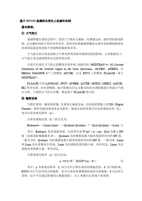
②辐射定标当我们拿到一幅原始影像,先要进行辐射定标,目的是把图像上的DN(Digital Number)值转为辐亮度或者是反射率。
辐射定标的结果可以是表观辐亮度(L),也可以是表观反射率(ρ)。
计算表观辐亮度(L)的公式为:Radiance=((Lmax-Lmin)/(Qcalmax-Qcalmin)*(Qcal-Qcalmin)+Lmin ①其中:Radiance 是表观辐亮度,注意单位是W/m2·sr·μm;Qcal为像元DN 值(也就是影像数据本身);Qcalmax为传感器处最大辐亮度值所对应的DN值,一般为255;Qcalmin 为传感器处最大辐亮度值所对应的DN值,一般为0;Lmax 和Lmin是从参数表中查询,Lmin为光谱辐亮度的最小值,单位同L;Lmax为光谱辐亮度的最大值,单位同L。
landsat5地表温度反演步骤
landsat5地表温度反演步骤
Landsat 5地表温度反演步骤如下:
1. 获取Landsat 5卫星遥感数据:从美国地质调查局(USGS)或其他相关机构获取相应的Landsat 5地表温度遥感数据。
2. 辐射校正:对遥感数据进行辐射校正,将数字计数值转换为辐射亮度。
3. 大气透过率校正:通过大气透过率模型校正遥感数据,去除大气影响。
4. 辐射温度计算:根据温度-辐射关系模型,将辐射亮度转换为辐射温度。
5. 地表辐射温度计算:考虑地表辐射率、植被覆盖、水汽含量等因素,将辐射温度转换为地表温度。
6. 数据剔除和补全:根据质量控制指标剔除无效数据,并进行缺失数据的补全。
7. 结果验证与分析:对反演结果进行验证和分析,与实地观测数据进行比较,并考虑地形、土壤类型等因素对结果进行解释和讨论。
8. 结果输出和应用:将地表温度反演结果输出为栅格数据或矢量数据,用于环境监测、气候研究、农业生产等应用领域。
需要注意的是,地表温度反演是一个复杂的过程,需要综合考虑多个因素,如大气状况、地表材料、遥感数据质量等,以确保反演结果的准确性和可靠性。
辐射定标,大气校正,辐射校正的区别与联系
辐射定标是进行遥感定量反演的一个前提,在遥感应用占有很重要的位置,下面部分内容主要摘自童庆禧先生的《高光谱遥感》辐射定标:建立遥感传感器的数字量化输出值DN与其所对应视场中辐射亮度值之间的定量关系。
1.实验室定标:在遥感器发射之前对其进行的波长位置、辐射精度、空间定位等的定标,将仪器的输出值转换为辐射值。
有的仪器内有内定定标系统。
但是在仪器运行之后,还需要定期定标,以监测仪器性能的变化,相应调整定标参数。
1光谱定标,其目的视确定遥感传感器每个波段的中心波长和带宽,以及光谱响应函数2辐射定标绝对定标:通过各种标准辐射源,在不同波谱段建立成像光谱仪入瞳处的光谱辐射亮度值与成像光谱仪输出的数字量化值之间的定量关系相对定标:确定场景中各像元之间、各探测器之间、各波谱之间以及不同时间测得的辐射量的相对值。
2.机上和星上定标机上定标用来经常性的检查飞行中的遥感器定标情况,一般采用内定标的方法,即辐射定标源、定标光学系统都在飞行器上,在大气层外,太阳的辐照度可以认为是一个常数,因此也可以选择太阳作为基准光源,通过太阳定标系统对星载成像光谱仪器进行绝对定标。
3.场地定标(是最难的一个)场地定标指的是遥感器处于正常运行条件下,选择辐射定标场地,通过地面同步测量对遥感器的定标,场地定标可以实现全孔径、全视场、全动态范围的定标,并考虑到了大气传输和环境的影响。
该定标方法可以实现对遥感器运行状态下与获取地面图像完全相同条件的绝对校正,可以提供遥感器整个寿命期间的定标,对遥感器进行真实性检验和对一些模型进行正确性检验。
但是地面目标应是典型的均匀稳定目标,地面定标还必须同时测量和计算遥感器过顶时的大气环境参量和地物反射率。
原理:在遥感器飞越辐射定标场地上空时,在定标场地选择偌干个像元区,测量成像光谱仪对应的地物的各波段光谱反射率和大气光谱等参量,并利用大气辐射传输模型等手段给出成像光谱仪入瞳处各光谱带的辐射亮度,最后确定它与成像光谱仪对应输出的数字量化值的数量关系,求解定标系数,并估算定标不确定性。
Landsat5TM数据辐射定标
( DN/( W·m-2·sr-1·μm-1) ) , B 是传感器偏置 ( DN) , Lλ是传感器 入瞳处的光谱辐射亮度( W/( m2·sr·μm) ) , 可见计算光谱辐射
亮度的关键在于确定 G 和 B。
Landsat 5 TM 长期以来一直采用基于星上内部定标灯的
辐射定标算法, 然而随着内部定标灯的逐渐老化, 定标精度
美国地质调查局( US GS ) 分别在 2003 年 5 月和 2007 年 4 月对其辐射定标算法进行了两次更新, 新算法采用基于查找表的定标算
法, 和 La nds a t 7 ETM+的定标算法相似。但是目前在遥感定量应用中对 TM 数据的辐射定标问题存在混乱状况, 影响了定标精度。
Байду номын сангаас
针对此状况, 对 La nds a t 5 TM 数据辐射定标问题进行了系统介绍, 重点分析了定标算法变化情况, 为正确进行 La nds a t 5 TM 数据
Landsat 5 卫星发射于 1984 年 3 月 1 日, 星上携带多光 谱 扫 描 仪 ( Multispectral Scanner, MSS) 和 专 题 制 图 仪 ( Thematic Mapper, TM) , 其 中 MSS 在 1992 年 底 停 止 接 收 数 据, TM 迄今一直正常运转, 积累了长达 24 a 的中分辨率对地 观测数据。TM 共有 7 个光谱波段, 其中 1 ̄5 和 7 波段是可见 光- 近红外波段, 空间分辨率为 30 m, 第 6 波段是热红外波 段 , 空 间 分 辨 率 为 120 m, 各 波 段 的 中 心 波 长 大 致 为 0.49, 0.56, 0.66, 0.83, 1.67, 11.5 和 2.24 μm。TM 的探测器共有 100 个, 分 7 个波段, 1 ̄5 和 7 波段探测器每组 16 个, 呈两行 错开排列, TM1 至 TM4 用硅探测器( 即 CCD 探 测 阵列 ) , TM5 和 TM7 各用 16 个锑化铟红外探测器, 其排列和 TM1 至 TM4 一样。TM6 用 4 个汞镉碲热红外探测器, 也成两行排列。TM1 至 TM5 及 TM7 每个探测器的瞬时视场在地面上为 30 m×30 m, TM6 为 120 m×120 m。
应用6S模型进行LANDSAT_TM影像大气校正

应用6S模型进行LANDSAT_TM影像大气校正应用6S 模型进行LANDSAT TM 影像大气校正一、辐射校正1、 1、用定标系数将原始DN 值转换为大气层顶太阳辐亮度L ;rescale cal rescale B Q G L +?=λL 为大气层顶太阳辐亮度,Q 为记录的电信号数值,rescaleG ,为通道增益,rescale B 为偏移量,定标系数可以在头文件中获得。
表1 LANDSAT5 TM 数据定标系数2、由大气层顶太阳辐亮度L 转换为反射率。
s p ESUN d L θπρλλcos 2=其中:pρ: 行星反射率λL : 传感器口径的光谱辐射值 d: 日地距离(以天文为单位)λESUN :Mean solar exoatmospheric irradiances 平均太阳外大气层辐射值s θ : 太阳天顶角表2 TM 太阳外大气层光谱辐射值表3,日地距离(以天文为单位)二、大气校正经过辐射校正后,象元灰度值转换为了反射率,我们使用6S模型对可见光和近红外波段进行大气校正。
1、辐射校正完的反射率是0-1之间的值,然后把它转换为0-100之间的数值;2、再在ENVI中把第一步中的反射率(0-100)存为RAW格式;3、然后在inputfiles中填写大气条件的输入文件、大气条件的输出文件名、待大气校正的输入文件(RAW格式)、待大气校正的图像大小;4、4、第3步中的大气条件的输入文件需要填写以下的几项:Landsat5 geometrical conditionsmonth,day,hh.ddd,long.,lat.tropical atmospheric modecontinental aerosols modelvisibility in km (aerosol model concentration)target at 600 m above sea levelsensor on board of satellitethird band of Landsat5the image has values of reflectance, DN is percent (actual values only 0-100, not 0-255)(-1)number of pixels of the image=number of bytes以上的这些参数可以根据实际情况进行填写。
ENVI-专题五LandsatTM辐射定标与大气纠正
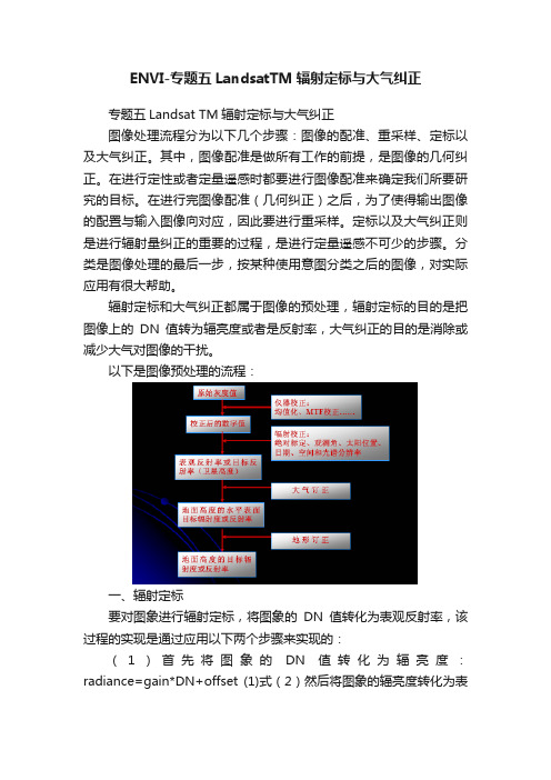
ENVI-专题五LandsatTM辐射定标与大气纠正专题五Landsat TM辐射定标与大气纠正图像处理流程分为以下几个步骤:图像的配准、重采样、定标以及大气纠正。
其中,图像配准是做所有工作的前提,是图像的几何纠正。
在进行定性或者定量遥感时都要进行图像配准来确定我们所要研究的目标。
在进行完图像配准(几何纠正)之后,为了使得输出图像的配置与输入图像向对应,因此要进行重采样。
定标以及大气纠正则是进行辐射量纠正的重要的过程,是进行定量遥感不可少的步骤。
分类是图像处理的最后一步,按某种使用意图分类之后的图像,对实际应用有很大帮助。
辐射定标和大气纠正都属于图像的预处理,辐射定标的目的是把图像上的DN值转为辐亮度或者是反射率,大气纠正的目的是消除或减少大气对图像的干扰。
以下是图像预处理的流程:一、辐射定标要对图象进行辐射定标,将图象的DN值转化为表观反射率,该过程的实现是通过应用以下两个步骤来实现的:(1)首先将图象的DN值转化为辐亮度:radiance=gain*DN+offset (1)式(2)然后将图象的辐亮度转化为表观反射率:(reflectance) ρ=π*L*d2/(ESUN*cos(θ))(2)式其中ρ为表观反射率,L为表观辐亮度,d为日地距离,ESUN为太阳平均辐射强度,θ为太阳天顶角。
(3)将以上两个步骤结合得:ρ=π*(gain*DN+offset)* d2/(ESUN*cos(θ))(3)式①日地天文单位距离D:D=1 - 0.01674 cos(0.9856× (JD-4)×π/180);JD为遥感成像的儒略日(Julian Day)D = 1 + 0.0167 * Sin(2 * PI * (days - 93.5) / 365);days是拍摄卫片的日期在那一年的天数,如2004年5月21号,则days=31+29+31+30+21=142。
计算得:D=1.01250756ENVI中的具体实现(以Landsat 7 ETM+为例):采用简单的波段运算例如,我们把2002-5-22的一幅ETM图像第3波段的DN值转化为表观反射率。
- 1、下载文档前请自行甄别文档内容的完整性,平台不提供额外的编辑、内容补充、找答案等附加服务。
- 2、"仅部分预览"的文档,不可在线预览部分如存在完整性等问题,可反馈申请退款(可完整预览的文档不适用该条件!)。
- 3、如文档侵犯您的权益,请联系客服反馈,我们会尽快为您处理(人工客服工作时间:9:00-18:30)。
Landsat TM 5辐射定标和大气校正(转)
2009-03-05 15:22
一、辐射定标
1. 由于ENVI 4.4 中有专门进行辐射定标的模块,因此实际的操作十分简单。
将原始TM 影像打开以后,选择
Basic Tools–Preprocessing–Calibration Utilities–Landsat TM
2. 进入下一步参数选择:根据传感器类型选择Landsat 4,5 或者7。
从遥感影像的头文件中获取Data Acquisition 的时间,Sun elevation。
如果你是用File–Open External File–Landsat–Fast 的方法打开header.dat 的话,sun elevation 就已经填好了。
这里Calibration Type 注意选择为Radiance。
输出文件,定标就完成了。
二、大气校正
简单一点的大气校正可以采用ENVI的FLAASH模块,以下就是FLAASH操作的步骤:
1. FLAASH 模块的进入方法是Spectral–FLAASH,或者是Basic
Tools–Preprocessing–Calibration Utilities–FLAASH。
2. FLAASH 模块的操作界面分为三块:最上部设定输入输出文件;中间设定传感器的参数;下部设定大气参数。
3. 首先设定输入输出文件。
FLAASH 模块要求输入辐亮度图像,输出反射率图像。
之前我们进行了辐射定标,得到辐亮度图像,在这里要把BSQ 格式的图像转换为BIL 或者BIP 格式的图像,然后再Input Radiance Image 中选择转换格式后的图像。
(Basic Tools–Convert Data(BSQ,BIL,BIP))。
这里注意,当输入图像后,程序会让你选择Scale Factor,即原始辐亮度单位与ENVI 默认辐亮度单位之间的比例。
ENVI 默认的辐亮度单位是μW/cm2 •sr•nm,而之前我们做辐射定标时单位是W/m2 •sr•μm,二者之间转换的比例是10,因此在下图中选择Single scale factor,填写10.000。
4. 此外,如果TM 影像的头文件中没有波段的信息,在这里也要求你提供一个.txt 文件以包含此信息。
那么,准备好一个.txt 文件,其中含有一列TM 每个波段中心波长的信息。
5. 在Output Reflectance File 和Output Directory for FLAASH files 里面设定输出文件的文件名和位置。
6. 设定传感器参数。
首先是Scene Center Location,即遥感图像中心的坐标,以及Flight Date, Flight Time GMT,这三者都可以在TM 的头文件中找到,填入即可。
7. 在Sensor Type 菜单中选择Landsat TM5。
此时Sensor altitude 自动填上
为705km。
而Pixel Size 填为30m。
8. 根据遥感影像研究区实际情况,填写Ground Elevation,比如华北平原可以写为0.05km。
9. 最关键的为大气参数部分:
a) Atmospheric Model( 大气模式): 共有Sub-Arctic Winter (SAW) ,
Mid-Latitude Winter (MLW),U.S. Standard (US) ,Sub-Arctic Summer(SAS), Mid-Latitude Summer (MLS) 和Tropical (T) 。
根据经纬度和时间可以选定研究区的大气模式,见ENVI Help。
b) Aerosol Model(气溶胶模式):有Rural, Urban, Maritime 和Tropospheric 四种选择。
根据实际情况选择即可。
关于此四种模式的解释见ENVI Help。
c) 当我们选择TM 时,可选的参数还有Aerosol Retrieval 和Initial Visibility。
这两个参数对最后的结果又相当重要的影像,因此最好能调查到当地的Initial Visibility。
此外,AERONET 在全世界各地有测定AOD(Atmospheric Optical Depth)的站点,可以查询AOD 以后转换为消光系数,通过消光系数估算能见度,此步骤比较繁琐,在此不予详述。
如果采用Aerosol Retrieval 中的K-T算法计算Visibility,且能够计算出结果的话,则采用K-T 算法的能见度,否
则采用Initial Visibility 所指定的能见度。
d) 关于Aerosol Retrieval。
如果选择了下拉菜单中的K-T method,那么需要在Multispectral Settings 中设定参数,在Assign Default Values Based on Retrieval Conditions 中选择Over-land Retrieval Standard (660:2100nm)即可。
根据不同的研究区可以设定不同的模式。
其他设定可以不改变。
Apply即可。