DSH Modelltest-Bauhaus Uni Weimar (LV+GR ohne Loesung)
Multi-scale structural similarity for image quality assesment
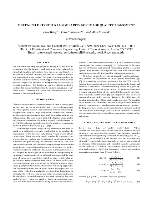
MULTI-SCALE STRUCTURAL SIMILARITY FOR IMAGE QUALITY ASSESSMENT Zhou Wang1,Eero P.Simoncelli1and Alan C.Bovik2(Invited Paper)1Center for Neural Sci.and Courant Inst.of Math.Sci.,New York Univ.,New York,NY10003 2Dept.of Electrical and Computer Engineering,Univ.of Texas at Austin,Austin,TX78712 Email:zhouwang@,eero.simoncelli@,bovik@ABSTRACTThe structural similarity image quality paradigm is based on the assumption that the human visual system is highly adapted for extracting structural information from the scene,and therefore a measure of structural similarity can provide a good approxima-tion to perceived image quality.This paper proposes a multi-scale structural similarity method,which supplies moreflexibility than previous single-scale methods in incorporating the variations of viewing conditions.We develop an image synthesis method to calibrate the parameters that define the relative importance of dif-ferent scales.Experimental comparisons demonstrate the effec-tiveness of the proposed method.1.INTRODUCTIONObjective image quality assessment research aims to design qual-ity measures that can automatically predict perceived image qual-ity.These quality measures play important roles in a broad range of applications such as image acquisition,compression,commu-nication,restoration,enhancement,analysis,display,printing and watermarking.The most widely used full-reference image quality and distortion assessment algorithms are peak signal-to-noise ra-tio(PSNR)and mean squared error(MSE),which do not correlate well with perceived quality(e.g.,[1]–[6]).Traditional perceptual image quality assessment methods are based on a bottom-up approach which attempts to simulate the functionality of the relevant early human visual system(HVS) components.These methods usually involve1)a preprocessing process that may include image alignment,point-wise nonlinear transform,low-passfiltering that simulates eye optics,and color space transformation,2)a channel decomposition process that trans-forms the image signals into different spatial frequency as well as orientation selective subbands,3)an error normalization process that weights the error signal in each subband by incorporating the variation of visual sensitivity in different subbands,and the vari-ation of visual error sensitivity caused by intra-or inter-channel neighboring transform coefficients,and4)an error pooling pro-cess that combines the error signals in different subbands into a single quality/distortion value.While these bottom-up approaches can conveniently make use of many known psychophysical fea-tures of the HVS,it is important to recognize their limitations.In particular,the HVS is a complex and highly non-linear system and the complexity of natural images is also very significant,but most models of early vision are based on linear or quasi-linear oper-ators that have been characterized using restricted and simplistic stimuli.Thus,these approaches must rely on a number of strong assumptions and generalizations[4],[5].Furthermore,as the num-ber of HVS features has increased,the resulting quality assessment systems have become too complicated to work with in real-world applications,especially for algorithm optimization purposes.Structural similarity provides an alternative and complemen-tary approach to the problem of image quality assessment[3]–[6].It is based on a top-down assumption that the HVS is highly adapted for extracting structural information from the scene,and therefore a measure of structural similarity should be a good ap-proximation of perceived image quality.It has been shown that a simple implementation of this methodology,namely the struc-tural similarity(SSIM)index[5],can outperform state-of-the-art perceptual image quality metrics.However,the SSIM index al-gorithm introduced in[5]is a single-scale approach.We consider this a drawback of the method because the right scale depends on viewing conditions(e.g.,display resolution and viewing distance). In this paper,we propose a multi-scale structural similarity method and introduce a novel image synthesis-based approach to calibrate the parameters that weight the relative importance between differ-ent scales.2.SINGLE-SCALE STRUCTURAL SIMILARITYLet x={x i|i=1,2,···,N}and y={y i|i=1,2,···,N}be two discrete non-negative signals that have been aligned with each other(e.g.,two image patches extracted from the same spatial lo-cation from two images being compared,respectively),and letµx,σ2x andσxy be the mean of x,the variance of x,and the covariance of x and y,respectively.Approximately,µx andσx can be viewed as estimates of the luminance and contrast of x,andσxy measures the the tendency of x and y to vary together,thus an indication of structural similarity.In[5],the luminance,contrast and structure comparison measures were given as follows:l(x,y)=2µxµy+C1µ2x+µ2y+C1,(1)c(x,y)=2σxσy+C2σ2x+σ2y+C2,(2)s(x,y)=σxy+C3σxσy+C3,(3) where C1,C2and C3are small constants given byC1=(K1L)2,C2=(K2L)2and C3=C2/2,(4)Fig.1.Multi-scale structural similarity measurement system.L:low-passfiltering;2↓:downsampling by2. respectively.L is the dynamic range of the pixel values(L=255for8bits/pixel gray scale images),and K1 1and K2 1aretwo scalar constants.The general form of the Structural SIMilarity(SSIM)index between signal x and y is defined as:SSIM(x,y)=[l(x,y)]α·[c(x,y)]β·[s(x,y)]γ,(5)whereα,βandγare parameters to define the relative importanceof the three components.Specifically,we setα=β=γ=1,andthe resulting SSIM index is given bySSIM(x,y)=(2µxµy+C1)(2σxy+C2)(µ2x+µ2y+C1)(σ2x+σ2y+C2),(6)which satisfies the following conditions:1.symmetry:SSIM(x,y)=SSIM(y,x);2.boundedness:SSIM(x,y)≤1;3.unique maximum:SSIM(x,y)=1if and only if x=y.The universal image quality index proposed in[3]corresponds to the case of C1=C2=0,therefore is a special case of(6).The drawback of such a parameter setting is that when the denominator of Eq.(6)is close to0,the resulting measurement becomes unsta-ble.This problem has been solved successfully in[5]by adding the two small constants C1and C2(calculated by setting K1=0.01 and K2=0.03,respectively,in Eq.(4)).We apply the SSIM indexing algorithm for image quality as-sessment using a sliding window approach.The window moves pixel-by-pixel across the whole image space.At each step,the SSIM index is calculated within the local window.If one of the image being compared is considered to have perfect quality,then the resulting SSIM index map can be viewed as the quality map of the other(distorted)image.Instead of using an8×8square window as in[3],a smooth windowing approach is used for local statistics to avoid“blocking artifacts”in the quality map[5].Fi-nally,a mean SSIM index of the quality map is used to evaluate the overall image quality.3.MULTI-SCALE STRUCTURAL SIMILARITY3.1.Multi-scale SSIM indexThe perceivability of image details depends the sampling density of the image signal,the distance from the image plane to the ob-server,and the perceptual capability of the observer’s visual sys-tem.In practice,the subjective evaluation of a given image varies when these factors vary.A single-scale method as described in the previous section may be appropriate only for specific settings.Multi-scale method is a convenient way to incorporate image de-tails at different resolutions.We propose a multi-scale SSIM method for image quality as-sessment whose system diagram is illustrated in Fig. 1.Taking the reference and distorted image signals as the input,the system iteratively applies a low-passfilter and downsamples thefiltered image by a factor of2.We index the original image as Scale1, and the highest scale as Scale M,which is obtained after M−1 iterations.At the j-th scale,the contrast comparison(2)and the structure comparison(3)are calculated and denoted as c j(x,y) and s j(x,y),respectively.The luminance comparison(1)is com-puted only at Scale M and is denoted as l M(x,y).The overall SSIM evaluation is obtained by combining the measurement at dif-ferent scales usingSSIM(x,y)=[l M(x,y)]αM·Mj=1[c j(x,y)]βj[s j(x,y)]γj.(7)Similar to(5),the exponentsαM,βj andγj are used to ad-just the relative importance of different components.This multi-scale SSIM index definition satisfies the three conditions given in the last section.It also includes the single-scale method as a spe-cial case.In particular,a single-scale implementation for Scale M applies the iterativefiltering and downsampling procedure up to Scale M and only the exponentsαM,βM andγM are given non-zero values.To simplify parameter selection,we letαj=βj=γj forall j’s.In addition,we normalize the cross-scale settings such thatMj=1γj=1.This makes different parameter settings(including all single-scale and multi-scale settings)comparable.The remain-ing job is to determine the relative values across different scales. Conceptually,this should be related to the contrast sensitivity func-tion(CSF)of the HVS[7],which states that the human visual sen-sitivity peaks at middle frequencies(around4cycles per degree of visual angle)and decreases along both high-and low-frequency directions.However,CSF cannot be directly used to derive the parameters in our system because it is typically measured at the visibility threshold level using simplified stimuli(sinusoids),but our purpose is to compare the quality of complex structured im-ages at visible distortion levels.3.2.Cross-scale calibrationWe use an image synthesis approach to calibrate the relative impor-tance of different scales.In previous work,the idea of synthesizing images for subjective testing has been employed by the“synthesis-by-analysis”methods of assessing statistical texture models,inwhich the model is used to generate a texture with statistics match-ing an original texture,and a human subject then judges the sim-ilarity of the two textures [8]–[11].A similar approach has also been qualitatively used in demonstrating quality metrics in [5],[12],though quantitative subjective tests were not conducted.These synthesis methods provide a powerful and efficient means of test-ing a model,and have the added benefit that the resulting images suggest improvements that might be made to the model[11].M )distortion level (MSE)12345Fig.2.Demonstration of image synthesis approach for cross-scale calibration.Images in the same row have the same MSE.Images in the same column have distortions only in one specific scale.Each subject was asked to select a set of images (one from each scale),having equal quality.As an example,one subject chose the marked images.For a given original 8bits/pixel gray scale test image,we syn-thesize a table of distorted images (as exemplified by Fig.2),where each entry in the table is an image that is associated witha specific distortion level (defined by MSE)and a specific scale.Each of the distorted image is created using an iterative procedure,where the initial image is generated by randomly adding white Gaussian noise to the original image and the iterative process em-ploys a constrained gradient descent algorithm to search for the worst images in terms of SSIM measure while constraining MSE to be fixed and restricting the distortions to occur only in the spec-ified scale.We use 5scales and 12distortion levels (range from 23to 214)in our experiment,resulting in a total of 60images,as demonstrated in Fig.2.Although the images at each row has the same MSE with respect to the original image,their visual quality is significantly different.Thus the distortions at different scales are of very different importance in terms of perceived image quality.We employ 10original 64×64images with different types of con-tent (human faces,natural scenes,plants,man-made objects,etc.)in our experiment to create 10sets of distorted images (a total of 600distorted images).We gathered data for 8subjects,including one of the authors.The other subjects have general knowledge of human vision but did not know the detailed purpose of the study.Each subject was shown the 10sets of test images,one set at a time.The viewing dis-tance was fixed to 32pixels per degree of visual angle.The subject was asked to compare the quality of the images across scales and detect one image from each of the five scales (shown as columns in Fig.2)that the subject believes having the same quality.For example,one subject chose the images marked in Fig.2to have equal quality.The positions of the selected images in each scale were recorded and averaged over all test images and all subjects.In general,the subjects agreed with each other on each image more than they agreed with themselves across different images.These test results were normalized (sum to one)and used to calculate the exponents in Eq.(7).The resulting parameters we obtained are β1=γ1=0.0448,β2=γ2=0.2856,β3=γ3=0.3001,β4=γ4=0.2363,and α5=β5=γ5=0.1333,respectively.4.TEST RESULTSWe test a number of image quality assessment algorithms using the LIVE database (available at [13]),which includes 344JPEG and JPEG2000compressed images (typically 768×512or similar size).The bit rate ranges from 0.028to 3.150bits/pixel,which allows the test images to cover a wide quality range,from in-distinguishable from the original image to highly distorted.The mean opinion score (MOS)of each image is obtained by averag-ing 13∼25subjective scores given by a group of human observers.Eight image quality assessment models are being compared,in-cluding PSNR,the Sarnoff model (JNDmetrix 8.0[14]),single-scale SSIM index with M equals 1to 5,and the proposed multi-scale SSIM index approach.The scatter plots of MOS versus model predictions are shown in Fig.3,where each point represents one test image,with its vertical and horizontal axes representing its MOS and the given objective quality score,respectively.To provide quantitative per-formance evaluation,we use the logistic function adopted in the video quality experts group (VQEG)Phase I FR-TV test [15]to provide a non-linear mapping between the objective and subjective scores.After the non-linear mapping,the linear correlation coef-ficient (CC),the mean absolute error (MAE),and the root mean squared error (RMS)between the subjective and objective scores are calculated as measures of prediction accuracy .The prediction consistency is quantified using the outlier ratio (OR),which is de-Table1.Performance comparison of image quality assessment models on LIVE JPEG/JPEG2000database[13].SS-SSIM: single-scale SSIM;MS-SSIM:multi-scale SSIM;CC:non-linear regression correlation coefficient;ROCC:Spearman rank-order correlation coefficient;MAE:mean absolute error;RMS:root mean squared error;OR:outlier ratio.Model CC ROCC MAE RMS OR(%)PSNR0.9050.901 6.538.4515.7Sarnoff0.9560.947 4.66 5.81 3.20 SS-SSIM(M=1)0.9490.945 4.96 6.25 6.98 SS-SSIM(M=2)0.9630.959 4.21 5.38 2.62 SS-SSIM(M=3)0.9580.956 4.53 5.67 2.91 SS-SSIM(M=4)0.9480.946 4.99 6.31 5.81 SS-SSIM(M=5)0.9380.936 5.55 6.887.85 MS-SSIM0.9690.966 3.86 4.91 1.16fined as the percentage of the number of predictions outside the range of±2times of the standard deviations.Finally,the predic-tion monotonicity is measured using the Spearman rank-order cor-relation coefficient(ROCC).Readers can refer to[15]for a more detailed descriptions of these measures.The evaluation results for all the models being compared are given in Table1.From both the scatter plots and the quantitative evaluation re-sults,we see that the performance of single-scale SSIM model varies with scales and the best performance is given by the case of M=2.It can also be observed that the single-scale model tends to supply higher scores with the increase of scales.This is not surprising because image coding techniques such as JPEG and JPEG2000usually compressfine-scale details to a much higher degree than coarse-scale structures,and thus the distorted image “looks”more similar to the original image if evaluated at larger scales.Finally,for every one of the objective evaluation criteria, multi-scale SSIM model outperforms all the other models,includ-ing the best single-scale SSIM model,suggesting a meaningful balance between scales.5.DISCUSSIONSWe propose a multi-scale structural similarity approach for image quality assessment,which provides moreflexibility than single-scale approach in incorporating the variations of image resolution and viewing conditions.Experiments show that with an appropri-ate parameter settings,the multi-scale method outperforms the best single-scale SSIM model as well as state-of-the-art image quality metrics.In the development of top-down image quality models(such as structural similarity based algorithms),one of the most challeng-ing problems is to calibrate the model parameters,which are rather “abstract”and cannot be directly derived from simple-stimulus subjective experiments as in the bottom-up models.In this pa-per,we used an image synthesis approach to calibrate the param-eters that define the relative importance between scales.The im-provement from single-scale to multi-scale methods observed in our tests suggests the usefulness of this novel approach.However, this approach is still rather crude.We are working on developing it into a more systematic approach that can potentially be employed in a much broader range of applications.6.REFERENCES[1] A.M.Eskicioglu and P.S.Fisher,“Image quality mea-sures and their performance,”IEEE munications, vol.43,pp.2959–2965,Dec.1995.[2]T.N.Pappas and R.J.Safranek,“Perceptual criteria for im-age quality evaluation,”in Handbook of Image and Video Proc.(A.Bovik,ed.),Academic Press,2000.[3]Z.Wang and A.C.Bovik,“A universal image quality in-dex,”IEEE Signal Processing Letters,vol.9,pp.81–84,Mar.2002.[4]Z.Wang,H.R.Sheikh,and A.C.Bovik,“Objective videoquality assessment,”in The Handbook of Video Databases: Design and Applications(B.Furht and O.Marques,eds.), pp.1041–1078,CRC Press,Sept.2003.[5]Z.Wang,A.C.Bovik,H.R.Sheikh,and E.P.Simon-celli,“Image quality assessment:From error measurement to structural similarity,”IEEE Trans.Image Processing,vol.13, Jan.2004.[6]Z.Wang,L.Lu,and A.C.Bovik,“Video quality assessmentbased on structural distortion measurement,”Signal Process-ing:Image Communication,special issue on objective video quality metrics,vol.19,Jan.2004.[7] B.A.Wandell,Foundations of Vision.Sinauer Associates,Inc.,1995.[8]O.D.Faugeras and W.K.Pratt,“Decorrelation methods oftexture feature extraction,”IEEE Pat.Anal.Mach.Intell., vol.2,no.4,pp.323–332,1980.[9] A.Gagalowicz,“A new method for texturefields synthesis:Some applications to the study of human vision,”IEEE Pat.Anal.Mach.Intell.,vol.3,no.5,pp.520–533,1981. [10] D.Heeger and J.Bergen,“Pyramid-based texture analy-sis/synthesis,”in Proc.ACM SIGGRAPH,pp.229–238,As-sociation for Computing Machinery,August1995.[11]J.Portilla and E.P.Simoncelli,“A parametric texture modelbased on joint statistics of complex wavelet coefficients,”Int’l J Computer Vision,vol.40,pp.49–71,Dec2000. [12]P.C.Teo and D.J.Heeger,“Perceptual image distortion,”inProc.SPIE,vol.2179,pp.127–141,1994.[13]H.R.Sheikh,Z.Wang, A. C.Bovik,and L.K.Cormack,“Image and video quality assessment re-search at LIVE,”/ research/quality/.[14]Sarnoff Corporation,“JNDmetrix Technology,”http:///products_services/video_vision/jndmetrix/.[15]VQEG,“Final report from the video quality experts groupon the validation of objective models of video quality assess-ment,”Mar.2000./.PSNRM O SSarnoffM O S(a)(b)Single−scale SSIM (M=1)M O SSingle−scale SSIM (M=2)M O S(c)(d)Single−scale SSIM (M=3)M O SSingle−scale SSIM (M=4)M O S(e)(f)Single−scale SSIM (M=5)M O SMulti−scale SSIMM O S(g)(h)Fig.3.Scatter plots of MOS versus model predictions.Each sample point represents one test image in the LIVE JPEG/JPEG2000image database [13].(a)PSNR;(b)Sarnoff model;(c)-(g)single-scale SSIM method for M =1,2,3,4and 5,respectively;(h)multi-scale SSIM method.。
扭力梁耐久等效台架试验设计及疲劳寿命预测方法
计算机辅助工程 Vcl.29 Nc.4Computee Aided EngineeringDec. 202029 42020 12文章编号:1"6 - 0871(2020)04-0016-06DOI : 10. 13340/j. cac. 2020. 04. 004扭力梁耐久等效台架试验设计及疲劳寿命预测方法余家皓,邓小强,郭绍良,朱冬冬(广川汽车集团股份有限公司汽车工程研究院,广川511434)摘要:针对传统扭力梁悬架开发中实车道路试验费用高、零部件迭代设计时间长的问题,根据传统疲劳寿命预测方法制定多轴载荷台架试验方案,利用试验测试和仿真手段对比的方法预测扭力梁 悬架寿命,分析基于应力叠加原理寿命估计方法的局限性,根据伪损伤等效原理提出更合理的寿命估计方法。
根据该方法设计等效台架试验方案,并进行有限元仿真和台架试验。
某扭力梁悬架开 发和整车耐久性试验证明该设计方法的有效性。
关键词:疲劳;耐久;等效;扭力梁;伪损伤中图分类号:TP391.92; U467.523 文献标志码:BEquivalent bench test scheme and life prediction method for twist beamYU Jiahao ,DENG Xiaoqiang ,GUO Shaoyang ,ZHU Dongdong(Automotive Research and Development Centee , Guangzhou Automobile Group Cc. , Ltd. , Guangzhou 511434, China )Abstract : As to the problems that the cost of road test is high and the parts design iteration time is long in traditional torsion beam suspension development , the multi 位xil load bench test scheme is plannedaeeoedingtotheteaditionaefatigueeifepeedietion method.Theeifeoftoesion beamsuspension ispeedieted by the comparison of test and simulation method. The limitation of lit estimation method based on stresssuperposition principle is analyzed , and a more reasonable lit estimation method is proposed according toth.ps.udodamag..quieaentpeineipe.Bas.d on thism.thod , th..quieaentb.neh tstseh.m.isdesigned , and the finite element simulation and bench Wst are carried out. The effectivenss of the design method is proved by the development of the torsion beam suspension and whole vehicle durability test.Key words : fatigue ; durability ; equivelence ; torsion beam ; pseudo damage0引言传统扭力梁开发需要进行实车道路试验和零部件迭代设计,开发需要的费用高、时间长。
yantubbs-The hardening soil model, Formulation and verification

The hardening soil model: Formulation and verificationT. SchanzLaboratory of Soil Mechanics, Bauhaus-University Weimar, GermanyP.A. VermeerInstitute of Geotechnical Engineering, University Stuttgart, GermanyP.G. BonnierP LAXIS B.V., NetherlandsKeywords: constitutive modeling, HS-model, calibration, verificationABSTRACT: A new constitutive model is introduced which is formulated in the framework of classical theory of plasticity. In the model the total strains are calculated using a stress-dependent stiffness, different for both virgin loading and un-/reloading. The plastic strains are calculated by introducing a multi-surface yield criterion. Hardening is assumed to be isotropic depending on both the plastic shear and volumetric strain. For the frictional hardening a non-associated and for the cap hardening an associated flow rule is assumed.First the model is written in its rate form. Therefor the essential equations for the stiffness mod-ules, the yield-, failure- and plastic potential surfaces are given.In the next part some remarks are given on the models incremental implementation in the P LAXIS computer code. The parameters used in the model are summarized, their physical interpre-tation and determination are explained in detail.The model is calibrated for a loose sand for which a lot of experimental data is available. With the so calibrated model undrained shear tests and pressuremeter tests are back-calculated.The paper ends with some remarks on the limitations of the model and an outlook on further de-velopments.1INTRODUCTIONDue to the considerable expense of soil testing, good quality input data for stress-strain relation-ships tend to be very limited. In many cases of daily geotechnical engineering one has good data on strength parameters but little or no data on stiffness parameters. In such a situation, it is no help to employ complex stress-strain models for calculating geotechnical boundary value problems. In-stead of using Hooke's single-stiffness model with linear elasticity in combination with an ideal plasticity according to Mohr-Coulomb a new constitutive formulation using a double-stiffness model for elasticity in combination with isotropic strain hardening is presented.Summarizing the existing double-stiffness models the most dominant type of model is the Cam-Clay model (Hashiguchi 1985, Hashiguchi 1993). To describe the non-linear stress-strain behav-iour of soils, beside the Cam-Clay model the pseudo-elastic (hypo-elastic) type of model has been developed. There an Hookean relationship is assumed between increments of stress and strain and non-linearity is achieved by means of varying Young's modulus. By far the best known model of this category ist the Duncan-Chang model, also known as the hyperbolic model (Duncan & Chang 1970). This model captures soil behaviour in a very tractable manner on the basis of only two stiff-ness parameters and is very much appreciated among consulting geotechnical engineers. The major inconsistency of this type of model which is the reason why it is not accepted by scientists is that, in contrast to the elasto-plastic type of model, a purely hypo-elastic model cannot consistently dis-tinguish between loading and unloading. In addition, the model is not suitable for collapse load computations in the fully plastic range.12These restrictions will be overcome by formulating a model in an elasto-plastic framework in this paper. Doing so the Hardening-Soil model, however, supersedes the Duncan-Chang model by far. Firstly by using the theory of plasticity rather than the theory of elasticity. Secondly by includ-ing soil dilatancy and thirdly by introducing a yield cap.In contrast to an elastic perfectly-plastic model, the yield surface of the Hardening Soil model is not fixed in principal stress space, but it can expand due to plastic straining. Distinction is made between two main types of hardening, namely shear hardening and compression hardening. Shear hardening is used to model irreversible strains due to primary deviatoric loading. Compression hardening is used to model irreversible plastic strains due to primary compression in oedometer loading and isotropic loading.For the sake of convenience, restriction is made in the following sections to triaxial loading conditions with 2σ′ = 3σ′ and 1σ′ being the effective major compressive stress.2 CONSTITUTIVE EQUATIONS FOR STANDARD DRAINED TRIAXIAL TESTA basic idea for the formulation of the Hardening-Soil model is the hyperbolic relationship be-tween the vertical strain ε1, and the deviatoric stress, q , in primary triaxial loading. When subjected to primary deviatoric loading, soil shows a decreasing stiffness and simultaneously irreversible plastic strains develop. In the special case of a drained triaxial test, the observed relationship be-tween the axial strain and the deviatoric stress can be well approximated by a hyperbola (Kondner& Zelasko 1963). Standard drained triaxial tests tend to yield curves that can be described by:The ultimate deviatoric stress, q f , and the quantity q a in Eq. 1 are defined as:The above relationship for q f is derived from the Mohr-Coulomb failure criterion, which involves the strength parameters c and ϕp . As soon as q = q f , the failure criterion is satisfied and perfectly plastic yielding occurs. The ratio between q f and q a is given by the failure ratio R f , which should obviously be smaller than 1. R f = 0.9 often is a suitable default setting. This hyperbolic relationship is plotted in Fig. 1.2.1 Stiffness for primary loadingThe stress strain behaviour for primary loading is highly nonlinear. The parameter E 50 is the con-fining stress dependent stiffness modulus for primary loading. E 50is used instead of the initial modulus E i for small strain which, as a tangent modulus, is more difficult to determine experimen-tally. It is given by the equation:ref E 50is a reference stiffness modulus corresponding to the reference stress ref p . The actual stiff-ness depends on the minor principal stress, 3σ′, which is the effective confining pressure in a tri-axial test. The amount of stress dependency is given by the power m . In order to simulate a loga-rithmic stress dependency, as observed for soft clays, the power should be taken equal to 1.0. As a3Figure 1. Hyperbolic stress-strain relation in primary loading for a standard drained triaxial test.secant modulus ref E 50 is determined from a triaxial stress-strain-curve for a mobilization of 50% ofthe maximum shear strength q f .2.2 Stiffness for un-/reloadingFor unloading and reloading stress paths, another stress-dependent stiffness modulus is used:where ref urE is the reference Young's modulus for unloading and reloading, corresponding to the reference pressure σ ref . Doing so the un-/reloading path is modeled as purely (non-linear) elastic.The elastic components of strain εe are calculated according to a Hookean type of elastic relation using Eqs. 4 + 5 and a constant value for the un-/reloading Poisson's ratio υur .For drained triaxial test stress paths with σ2 = σ3 = constant, the elastic Young's modulus E ur re-mains constant and the elastic strains are given by the equations:Here it should be realised that restriction is made to strains that develop during deviatoric loading,whilst the strains that develop during the very first stage of the test are not considered. For the first stage of isotropic compression (with consolidation), the Hardening-Soil model predicts fully elastic volume changes according to Hooke's law, but these strains are not included in Eq. 6.2.3 Yield surface, failure condition, hardening lawFor the triaxial case the two yield functions f 12 and f 13 are defined according to Eqs. 7 and 8. Here4Figure 2. Successive yield loci for various values of the hardening parameter γ p and failure surface.the measure of the plastic shear strain γ p according to Eq. 9 is used as the relevant parameter forthe frictional hardening:with the definitionIn reality, plastic volumetric strains p υε will never be precisely equal to zero, but for hard soils plastic volume changes tend to be small when compared with the axial strain, so that the approxi-mation in Eq. 9 will generally be accurate.For a given constant value of the hardening parameter, γ p , the yield condition f 12 = f 13 = 0 can be visualised in p'-q-plane by means of a yield locus. When plotting such yield loci, one has to use Eqs. 7 and 8 as well as Eqs. 3 and 4 for E 50 and E ur respectively. Because of the latter expressions,the shape of the yield loci depends on the exponent m . For m = 1.0 straight lines are obtained, but slightly curved yield loci correspond to lower values of the exponent. Fig. 2 shows the shape of successive yield loci for m = 0.5, being typical for hard soils. For increasing loading the failure sur-faces approach the linear failure condition according to Eq. 2.2.4 Flow rule, plastic potential functionsHaving presented a relationship for the plastic shear strain, γ p , attention is now focused on the plastic volumetric strain p υε. As for all plasticity models, the Hardening-Soil model involves a re-lationship between rates of plastic strain, i.e. a relationship between p υε and p γ . This flow rule hasthe linear form:5Clearly, further detail is needed by specifying the mobilized dilatancy angle m ψ. For the presentmodel, the expression:is adopted, where cv ϕ is the critical state friction angle, being a material constant independent ofdensity (Schanz & Vermeer 1996), and m ϕ is the mobilized friction angle:The above equations correspond to the well-known stress-dilatancy theory (Rowe 1962, Rowe 1971), as explained by (Schanz & Vermeer 1996). The essential property of the stress-dilatancy theory is that the material contracts for small stress ratios m ϕ < cv ϕ, whilst dilatancy occurs for high stress ratios m ϕ < cv ϕ. At failure, when the mobilized friction angle equals the failure angle,p ϕ, it is found from Eq. 11 that:Hence, the critical state angle can be computed from the failure angles p ϕand p ψ. The above defi-nition of the flow rule is equivalent to the definition of definition of the plastic potential functionsg 12 and g 13 according to:Using theKoiter-rule (Koiter 1960) for yielding depending on two yield surfaces (Multi-surface plasticity ) one finds:Calculating the different plastic strain rates by this equation, Eq. 10 directly follows.3 TIME INTEGRATIONThe model as described above has been implemented in the finite element code P LAXIS (Vermeer& Brinkgreve 1998). To do so, the model equations have to be written in incremental form. Due to this incremental formulation several assumptions and modifications have to be made, which will be explained in this section.During the global iteration process, the displacement increment follows from subsequent solu-tion of the global system of equations:where K is the global stiffness matrix in which we use the elastic Hooke's matrix D , f ext is a global load vector following from the external loads and f int is the global reaction vector following from the stresses. The stress at the end of an increment σ 1 can be calculated (for a given strain increment ∆ε) as:6whereσ0 , stress at the start of the increment,∆σ , resulting stress increment,4D , Hooke's elasticity matrix, based on the unloading-reloading stiffness,∆ε , strain increment (= B ∆u ),γ p , measure of the plastic shear strain, used as hardening parameter,∆Λ , increment of the non-negative multiplier,g , plastic potential function.The multiplier Λ has to be determined from the condition that the function f (σ1, γ p ) = 0 has to be zero for the new stress and deformation state.As during the increment of strain the stresses change, the stress dependant variables, like the elasticity matrix and the plastic potential function g , also change. The change in the stiffness during the increment is not very important as in many cases the deformations are dominated by plasticity.This is also the reason why a Hooke's matrix is used. We use the stiffness matrix 4D based on the stresses at the beginning of the step (Euler explicit ). In cases where the stress increment follows from elasticity alone, such as in unloading or reloading, we iterate on the average stiffness during the increment.The plastic potential function g also depends on the stresses and the mobilized dilation angle m ψ. The dilation angle for these derivatives is taken at the beginning of the step. The implementa-tion uses an implicit scheme for the derivatives of the plastic potential function g . The derivatives are taken at a predictor stress σtr , following from elasticity and the plastic deformation in the previ-ous iteration:The calculation of the stress increment can be performed in principal stress space. Therefore ini-tially the principal stresses and principal directions have to be calculated from the Cartesian stresses, based on the elastic prediction. To indicate this we use the subscripts 1, 2 and 3 and have 321σσσ≥≥ where compression is assumed to be positive.Principal plastic strain increments are now calculated and finally the Cartesian stresses have to be back-calculated from the resulting principal constitutive stresses. The calculation of the consti-tutive stresses can be written as:From this the deviatoric stress q (σ1 – σ3) and the asymptotic deviatoric stress q a can be expressed in the elastic prediction stresses and the multiplier ∆Λ:7whereFor these stresses the functionshould be zero. As the increment of the plastic shear strain ∆γ p also depends linearly on the multi-plier ∆Λ, the above formulae result in a (complicated) quadratic equation for the multiplier ∆Λwhich can be solved easily. Using the resulting value of ∆Λ, one can calculate (incremental)stresses and the (increment of the) plastic shear strain.In the above formulation it is assumed that there is a single yield function. In case of triaxial compression or triaxial extension states of stress there are two yield functions and two plastic po-tential functions. Following (Koiter 1960) one can write:where the subscripts indicate the principal stresses used for the yield and potential functions. At most two of the multipliers are positive. In case of triaxial compression we have σ2 = σ3, Λ23 = 0and we use two consistency conditions instead of one as above. The increment of the plastic shear strain has to be expressed in the multipliers. This again results in a quadratic equation in one of the multipliers.When the stresses are calculated one still has to check if the stress state violates the yield crite-rion q ≤ q f . When this happens the stresses have to be returned to the Mohr-Coulomb yield surface.4 ON THE CAP YIELD SURFACEShear yield surfaces as indicated in Fig. 2 do not explain the plastic volume strain that is measured in isotropic compression. A second type of yield surface must therefore be introduced to close the elastic region in the direction of the p-axis. Without such a cap type yield surface it would not be possible to formulate a model with independent input of both E 50 and E oed . The triaxial modulus largely controls the shear yield surface and the oedometer modulus controls the cap yield surface.In fact, ref E 50largely controls the magnitude of the plastic strains that are associated with the shear yield surface. Similarly, ref oedE is used to control the magnitude of plastic strains that originate from the yield cap. In this section the yield cap will be described in full detail. To this end we consider the definition of the cap yield surface (a = c cot ϕ):8where M is an auxiliary model parameter that relates to NC K 0 as will be discussed later. Further more we have p = (σ1 + σ2+ σ3) andwithq is a special stress measure for deviatoric stresses. In the special case of triaxial compression it yields q = (σ1 – σ3) and for triaxial extension reduces to q = α (σ1 –σ3). For yielding on the cap surface we use an associated flow rule with the definition of the plastic potential g c :The magnitude of the yield cap is determined by the isotropic pre-consolidation stress p c . For the case of isotropic compression the evolution ofp c can be related to the plastic volumetric strain rate p v ε:Here H is the hardening modulus according to Eq. 32, which expresses the relation between theelastic swelling modulus K s and the elasto-plastic compression modulus K c for isotropic compres-sion:From this definition follows a stress dependency of H . For the case of isotropic compression we haveq = 0 and therefor c p p=. For this reason we find Eq. 33 directly from Eq. 31:The plastic multiplier c Λ referring to the cap is determined according to Eq. 35 using the addi-tional consistency condition:Using Eqs. 33 and 35 we find the hardening law relating p c to the volumetric cap strain c v ε:9Figure 3. Representation of total yield contour of the Hardening-Soil model in principal stress space for co-hesionless soil.The volumetric cap strain is the plastic volumetric strain in isotropic compression. In addition to the well known constants m and σref there is another model constant H . Both H and M are cap pa-rameters, but they are not used as direct input parameters. Instead, we have relationships of theform NC K 0=NC K 0(..., M, H ) and ref oed E = ref oed E (..., M, H ), such that NC K 0and ref oed E can be used as in-put parameters that determine the magnitude of M and H respectively. The shape of the yield cap is an ellipse in p – q ~-plane. This ellipse has length p c + a on the p -axis and M (p c+ a ) on the q ~-axis.Hence, p c determines its magnitude and M its aspect ratio. High values of M lead to steep caps un-derneath the Mohr-Coulomb line, whereas small M -values define caps that are much more pointed around the p -axis.For understanding the yield surfaces in full detail, one should consider Fig. 3 which depicts yield surfaces in principal stress space. Both the shear locus and the yield cap have the hexagonal shape of the classical Mohr-Coulomb failure criterion. In fact, the shear yield locus can expand up to the ultimate Mohr-Coulomb failure surface. The cap yield surface expands as a function of the pre-consolidation stress p c .5 PARAMETERS OF THE HARDENING-SOIL MODELSome parameters of the present hardening model coincide with those of the classical non-hardening Mohr-Coulomb model. These are the failure parameters ϕp ,, c and ψp . Additionally we use the ba-sic parameters for the soil stiffness:ref E 50, secant stiffness in standard drained triaxial test,ref oedE , tangent stiffness for primary oedometer loading and m , power for stress-level dependency of stiffness.This set of parameters is completed by the following advanced parameters:ref urE , unloading/ reloading stiffness,10v ur , Poisson's ratio for unloading-reloading,p ref , reference stress for stiffnesses,NC K 0, K 0-value for normal consolidation andR f , failure ratio q f / q a .Experimental data on m , E 50 and E oed for granular soils is given in (Schanz & Vermeer 1998).5.1 Basic parameters for stiffnessThe advantage of the Hardening-Soil model over the Mohr-Coulomb model is not only the use of a hyperbolic stress-strain curve instead of a bi-linear curve, but also the control of stress level de-pendency. For real soils the different modules of stiffness depends on the stress level. With theHardening-Soil model a stiffness modulus ref E 50is defined for a reference minor principal stress of σ3 = σref . As some readers are familiar with the input of shear modules rather than the above stiff-ness modules, shear modules will now be discussed. Within Hooke's theory of elasticity conversion between E and G goes by the equation E = 2 (1 + v ) G . As E ur is a real elastic stiffness, one may thus write E ur = 2 (1 + v ur ) G ur , where G ur is an elastic shear modulus. In contrast to E ur , the secant modulus E 50 is not used within a concept of elasticity. As a consequence, there is no simple conver-sion from E 50 to G 50. In contrast to elasticity based models, the elasto-plastic Hardening-Soil model does not involve a fixed relationship between the (drained) triaxial stiffness E 50 and the oedometer stiffness E oed . Instead, these stiffnesses must be given independently. To define the oedometer stiff-ness we usewhere E oed is a tangent stiffness modulus for primary loading. Hence, ref oed E is a tangent stiffness ata vertical stress of σ1 = σref .5.2 Advanced parametersRealistic values of v ur are about 0.2. In contrast to the Mohr-Coulomb model, NC K 0 is not simply a function of Poisson's ratio, but a proper input parameter. As a default setting one can use the highly realistic correlation NC K 0= 1 – sin ϕp . However, one has the possibility to select different values.All possible different input values for NC K 0 cannot be accommodated for. Depending on other pa-rameters, such as E 50, E oed , E ur and v ur , there happens to be a lower bound on NC K 0. The reason for this situation will be explained in the next section.5.3 Dilatancy cut-offAfter extensive shearing, dilating materials arrive in a state of critical density where dilatancy has come to an end. This phenomenon of soil behaviour is included in the Hardening-Soil model by means of a dilatancy cut-off . In order to specify this behaviour, the initial void ratio, e 0, and the maximum void ratio, e cv , of the material are entered. As soon as the volume change results in a state of maximum void, the mobilized dilatancy angle, ψm , is automatically set back to zero, as in-dicated in Eq. 38 and Fig. 4:11Figure 4. Resulting strain curve for a standard drained triaxial test including dilatancy cut-off.The void ratio is related to the volumetric strain, εv by the relationship:where an increment of εv is negative for dilatancy. The initial void ratio, e 0, is the in-situ void ratio of the soil body. The maximum void ratio, e cv , is the void ratio of the material in a state of critical void (critical state).6 CALIBRATION OF THE MODELIn a first step the Hardening-Soil model was calibrated for a sand by back-calculating both triaxial compression and oedometer tests. Parameters for the loosely packed Hostun-sand (e 0 = 0.89), a well known granular soil in geotechnical research, are given in Tab. 1. Figs. 5 and 6 show the satis-fying comparison between the experimental (three different tests) and the numerical result. For the oedometer tests the numerical results consider the unloading loop at the maximum vertical load only.7 VERIFICATION OF THE MODEL7.1 Undrained behaviour of loose Hostun-sandIn order to verify the model in a first step two different triaxial compression tests on loose Hostun-sand under undrained conditions (Djedid 1986) were simulated using the identical parameter from the former calibration. The results of this comparison are displayed in Figs. 7 and 8.In Fig. 7 we can see that for two different confining pressures of σc = 300 and 600 kPa the stress paths in p-q-space coincide very well. For deviatoric loads of q ≈ 300 kPa excess porewater pres-sures tend to be overestimated by the calculations.Additionally in Fig. 8 the stress-strain-behaviour is compared in more detail. This diagram con-tains two different sets of curves. The first set (•, ♠) relates to the axial strain ε1 at the horizontal12Figure 5. Comparison between the numerical (•) and experimental results for the oedometer tests.Figure 6. Comparison between the numerical (•) and experimental results for the drained triaxial tests (σ3 = 300 kPa) on loose Hostun-sand.and the effective stress ratio 31/σσ′′ on the vertical (left) axis. The second set (o , a ) refers to the normalised excess pore water pressure ∆u /σc on the right vertical axis. Experimental results forboth confining stresses are marked by symbols, numerical results by straight and dotted lines.Analysing the amount of effective shear strength it can be seen that the maximum calculated stress ratio falls inside the range of values from the experiments. The variation of effective friction from both tests is from 33.8 to 35.4 degrees compared to an input value of 34 degrees. Axial stiff-ness for a range of vertical strain of ε1 < 0.05 seems to be slightly over-predicted by the model. Dif-ferences become more pronounced for the comparison of excess pore water pressure generation.Here the calculated maximum amount of ∆u is higher then the measured values. The rate of de-crease in ∆u for larger vertical strain falls in the range of the experimental data.Table 1. Parameters of loose Hostun-sand.v urm ϕp ψp ref ref s E E 50/ref ref ur E E 50/ref E 500.200.6534° 0° 0.8 3.0 20 MPa13Figure 7. Undrained behaviour of loose Hostun-sand: p-q-plane.Figure 8. Undrained behaviour of loose Hostun-sand: stress-strain relations.7.2 Pressuremeter test GrenobleThe second example to verify the Hardening-Soil model is a back-calculation of a pressuremeter test on loose Hostun-sand. This test is part of an experimental study using the calibration chamber at the IMG in Grenoble (Branque 1997). This experimental testing facility is shown in Fig. 9.The cylindrical calibration chamber has a height of 150 cm and a diameter of 120 cm. In the test considered in the following a vertical surcharge of 500 kPa is applied at the top of the soil mass by a membrane. Because of the radial deformation constraint the state of stress can be interpreted in this phase as under oedometer conditions. Inside the chamber a pressuremeter sonde of a radius r 0 of 2.75 cm and a length of 16 cm is placed. For the test considered in the following example there was loose Hostun-sand (D r ≈ 0.5) of a density according to the material parameters as shown in Tab. 1 placed around the pressuremeter by pluviation. After the installation of the device and the filling of the chamber the pressure is increased and the resulting volume change is registered.14Figure 9. Pressuremeter Grenoble .This experimental setup was modeled within a FE-simulation as shown in Fig. 10. On the left hand side the axis-symmetric mesh and its boundary conditions is displayed. The dimensions are those of the complete calibration chamber. In the left bottom corner of the geometry the mesh is finer because there the pressuremeter is modeled.In the first calculation phase the vertical surcharge load A is applied. At the same time the hori-zontal load B is increased the way practically no deformations occur at the free deformation bound-ary in the left bottom corner. In the second phase the load group A is kept constant and the load group B is increased according to the loading history in the experiment. The (horizontal) deforma-tions are analysed over the total height of the free boundary. In order to (partly) get rid of the de-formation constrains at the top of this boundary, marked point A in the detail on the right hand side of Fig. 10 two interfaces were placed crossing each other in point A . Fig. 11 shows the comparison of the experimental and numerical results for the test with a vertical surcharge of 500 kPa.On the vertical axis the pressure (relating to load group B ) is given and on the horizontal axis the volumetric deformation of the pressuremeter. Because the calculation was run taking into ac-count large deformations (updated mesh analysis ) the pressure p in the pressuremeter has to be cal-culated from load multiplier ΣLoad B according to Eq. 40, taking into account the mean radial de-formation ∆r of the free boundary:The agreement between the experimental and the numerical data is very good, both for the initial part of phase 2 and for larger deformations of up to 30%.。
弹性薄膜可视化检测系统

弹性薄膜可视化检测系统由于人工检视员缺少客观可靠的途径来决定工件缺陷的存在与否,因此对宽四英尺、周长八英尺的弹性带的人工检查十分困难。
总体上来讲,工件的缺陷是指比周围材料颜色更暗或更亮的区域。
位于迈阿密斯堡的Invotec 工程处被生产弹性薄膜带的公司询问,机器检查是否可以用来制定一个客观的规格体系,从而可以多次提供检查结果。
Invoctec 的工程师们同客户合作,共同研发了一套规格体系,同时考虑到了工件的尺寸、过亮或过暗区域,以及缺陷同周围材料的反差。
这一方法与两台Cognex In-Sight 5000 系列视觉系统一起实现了自动化,在16 秒内完全检查了一个薄膜带。
系统在工件的不同区域截取了几幅图像。
开始的几幅图是用来调整出适当的增量,来补偿薄膜由于在摄影机前面旋转而造成的可能的工件厚度变化。
Invotec 的副总裁兼技术指导—达瑞尔格雷维特说:“我们在机械可视参数的基础上研发了这套客观的规格体系,同时展示了在此规格系统上建立的可重复操作的工件检查能力,从而实现了快速的完全检查。
”确保重要组成部分质量的挑战由于弹性薄膜是应用于医疗器械,因此严格剔除存在针孔、薄的斑点、内含物和嵌入粒子的工件显得尤为重要。
以前,这些缺陷都是由人工检查的,通过背光处理并将该薄膜夹在两个锭中间旋转,然后由检查员寻找缺陷。
自然地人工视觉意味着如果存在一定的明显缺陷,每个检查员都能检查得出。
然而仍然存在许多小缺陷或细微变化,一些检查员认为这是一个缺陷,而另一些检查员认为它不是缺陷。
许多检查员甚至前一天通过了一个存在微小缺陷的工件,而第二天又将它剔除。
薄膜的生产厂家要求Invotec 参与这样一个工程,因为该公司在机械视觉应用方面有着广泛的经验。
Inovtec 为客户提供设计装配、检测和试验系统,同时为许多不同制造业的制造公司提供工装、工具和量规。
Invotec 的工程师选取Cognex 的。
扩展式多次项自由曲面检测方法与流程

扩展式多次项自由曲面检测方法与流程Expanding the multiple term free-form surface detection method is a crucial aspect of computer-aided design and manufacturing. With the increasing demand for complex and organic shapes in various industries, it is important to have advanced techniques to accurately detect and analyze these surfaces. One of the key challenges in this area is the detection of complex curves and surfaces that include multiple terms in their equations. These surfaces are often found in applications such as automotive design, aerospace engineering, and medical device manufacturing. As such, developing a robust method for detecting these surfaces is essential for ensuring the quality and accuracy of the final product.扩展多次项自由曲面检测方法对计算机辅助设计和制造是至关重要的。
随着各行业对复杂和有机形状的需求不断增加,有必要使用先进技术来准确检测和分析这些曲面。
在这一领域的一个关键挑战是检测包含多项式的复杂曲线和曲面。
Autodesk CFD软件使用教程:建筑火灾和烟雾模拟说明书

BLD 195948Autodesk CFD for Fire and Smoke Simulation in BuildingsDr. Munirajulu. ML&T Construction, Larsen & Toubro LimitedDescriptionThis class will cover the use of Autodesk CFD software as a design analysis tool for fire and smoke simulation in buildings. We will examine how fire contaminant and smoke generation is modeled, and take you through the procedures and techniques necessary to obtain an efficient solution. You will learn how to identify design risk from the results visualization of smoke and temperature from the simulation. We will show you how to evaluate smoke-free height, tenable temperature, and smoke visibility to meet life-safety goals. Based on the Autodesk CFD results, you will understand how you can gain insight into behavior of smoke from fire, and make good design decisions to minimize smoke hazards. We will also highlight benefits and limitations of smoke simulation in relation to real-world fire scenarios. Finally, you will be able to relate the procedures and techniques described here for large spaces such as atria, convention centers, shopping malls, exhibition halls, airport terminals, and sports arenas.SpeakerDr. Munirajulu. M, B.Tech and Ph.D. from IIT, Kharagpur, India, has more than 22 years of direct and indirect involvement with CFD technology as a design analysis tool in areas such as HVAC, Automotive, Fluid Handling Equipment, Steam turbines and boilers. He has been with Larsen & Toubro Limited since 2005 and prior to this, he has worked with ABB Limited and Alstom Projects India Limited for about 9 years. His professional interests include state of the art CAE technologies (CAD, CFD and FEA). Currently he is responsible for CFD analysis in MEP design related to commercial buildings and airports in L&T Construction, Larsen & Toubro Limited, Chennai. He has been using Autodesk CFD Simulation software for HVAC and MEP applications in areas such as thermal comfort, data center cooling, basement car park ventilation, DG room ventilation effectiveness, rain water free surface flow for roof design, and smoke simulation in buildings in design stage as well as for trouble shooting. He has published 4 nos. of technical papers in international journals of repute and has been a speaker at technical conferences including AU 2017.Learning Objectives• Learn how fire and smoke is modeled • Visualize and Highlight key results• Gain insight into making good design decisions • Understand Benefits and limitationsContentsAutodesk CFD for Fire and Smoke Simulation in Buildings (1)Key word– Life Safety. (4)Back to basics (4)Fire Triangle/ Tetrahedron (4)Stages of fire (5)How fire spreads (6)Effects of uncontrolled fire (7)Hot smoke and life safety—what does temperature do? (7)Smoke contaminant and life safety – what does smoke do? (8)Loss due to fire (8)Objective 1: Fire and smoke modeling using Autodesk CFD (9)Fire safety strategy (9)Codes / standards used (9)General practice of smoke simulation (10)Building geometry: Retail shopping mall (11)Material properties (12)Boundary conditions (13)Mesh details (14)Initial conditions (15)Solver settings (15)Objective 2: Key results for final design (16)What do we look for in CFD analysis? (16)Smoke development (17)Key result 1: Smoke visibility (18)Temperature development (19)Key Result 2: Smoke temperature (20)Air flow field development (20)Key result 3: Air flow field (21)Outcome for final design (22)Objective 3: Insights from CFD analysis for good design decisions (22)Challenges in design..... . (22)Comparison of smoke control zones (23)Comparison of smoke visibility (24)Comparison of smoke temperature (25)Comparison of air/smoke flow field (25)Optimize smoke exhaust system design... summary . (26)More examples: (27)Objective 4: Benefits and limitations (27)Benefits: (27)Limitations: (27)Key word– Life Safety.We are going to look at what would ensure safety of people in a Retail shopping mallbuilding based on CFD analysis to understand smoke and temperature development in the event of fire.Back to basicsBefore we jump into the fire modeling using CFD, let us look at some basics •Fire triangle/ tetrahedron•Stages of fire•What is fire dynamics? How does fire spread?Fire Triangle/ Tetrahedron•The fire triangle identifies thethree needed components offire:•fuel (something that will burn)•heat (enough to make the fuelburn)•and air (oxygen)• a fourth component – theuninhibited chain reaction/news-and-research/news-and-media/press-room/reporters-guide-to-fire-and-nfpa/all-about-fireFire Triangle – Controlled firehttps:///wiki/Fire_triangleFire Tetrahedron – Uncontrolled fireStages of fire•Ignition: Fuel, oxygen andheat join together in asustained chemical reaction.•Growth: With the initial flameas a heat source, additionalfuel ignites. The size of the fireincreases and the plumereaches the ceiling.•Fully developed: Fire hasspread over much of fuel;temperatures reach their peak•Decay (burnout): The fireconsumes available fuel,temperatures decrease, firegets less intense.How fire spreadsFire spreads by transferring the heat energy from the flames in three different ways: - •Conduction: The passage of heat energy through or within a material because of direct contact, such as a burning wastebasket heating a nearby couch, which ignites and heats the drapes hanging behind, until they too burst into flames.•Convection: The flow of fluid or gas from hot areas to cooler areas.•Radiation: Heat traveling via electromagnetic waves, without objects or gases carrying it along. Radiated heat goes out in all directions, unnoticed until it strikes an object.ConductionConvectionhttps:///%3Cfront%3E/fire-dynamicsRadiationEffects of uncontrolled fire•Human loss•Structural damage•Material damage•Disruption of work•Financial lossesHot smoke and life safety—what does temperature do?https:///%3Cfront%3E/fire-dynamicsSmoke contaminant and life safety – what does smoke do?/news-and-research/news-and-media/press-room/reporters-guide-to-fire-and-nfpa/consequences-of-fire#fumesLoss due to fireHaving gone through certain relevant information about fire and facts about consequences of fire in terms of personal and economic loss, we will now get into details about how Autodesk CFD simulation can be useful in evaluating smoke spread and temperature distribution in a Retail mall building with a view to validate smoke exhaust system design for life safety. Objective 1: Fire and smoke modelling using Autodesk CFDFire safety strategyEngineering based approach to fire safe design:•Automatic fire detection (Smoke & heat detectors) - beam detectors in atrium/skylight areas and point type detectors in occupied areas•Automatic alarm system•Automatic fire sprinkler system for fire suppression•Exit signage•Smoke control – make up air and smoke extract fans•Egress – available safe egress time based on NFPA 101•Smoke zones - designed to restrict smoke from spreading from one smoke zone to another•Fire detection system - zoned identical to the smoke zones, including all visual and audible fire alarms.•Fire sprinkler system - zoned similar to the smoke zones and vice versa throughout the building.Codes / standards used•National Building Code (NBC 2005) of India•NFPA 101 Life Safety Code (2006)•NFPA 92 B - Standard for Smoke-control systems (2012 )•BS PD 7974-6:2004General practice of smoke simulation Flow only enters andleaves through thebottom and top surfaces.The main flow directionshould be to the vertical.Gap underneath the firefor cool air to be drawn inBuilding geometry: Retail shopping mallSectional details of the Retail mallMaterial propertiesAir : Variable quantity, to account for density variation with temperature and buoyancy Fire PartUse free arearatio =0.85 andconductivity of200 W/m-K tospread the heatwithin the flameFire modelled as a short cylinder and assigned as resistance material.Steel ring around the fire part (~1/2 flame height) and suppressed fromthe meshFast t- squared fire growth up to 2500 kW and steady state thereafter is considered, Firediameter = 3.35 m (NFPA 92B, A.5.2.1, based on HRRPUA 568 kW/m 2 and fire size of 5 MW). Variation of fire size with respect to time. Fire size reaches 1.75 MW (convective portion of 2.5 MW) at 210 seconds. Convective portion is taken as 70% of the total fire HRR.Boundary conditionsInlet boundary conditions – air domain inlet ambient temperature, scalar and pressureOutlet boundary conditions --smoke exhaust fan capacitiesMesh detailsThe fire and the air above and below - good uniform mesh- to capture the flow accurately by CFDFire sourceSolid ring suppressed from the mesh and ensures that flow only enters and leaves through the bottom and top surfacesInitial conditionsAir domain set at initial conditions as scalar = 0, temperature = 35.20 CSolver settingsObjective 2: Key results for final designWhat do we look for in CFD analysis?For designers and regulators, information about• Smoke movement• Temperature distribution• Airflow fieldSmoke transport is tracked w.r.t rise of smoke in atrium, along corridors and interconnected spacesKey results to look for :• Smoke free space• Tenable smoke temperatureBased on BS PD 7974-6:2004, Annex G•Smoke tenability limit - 10m visibility, Table G.1•Temperature tenability limit - 600C, Table G.3•Toxicity is deemed acceptable if visibility >10mSmoke developmentSmoke visibility (Smoke free space) – X PlaneSmoke visibility (Smoke free space) – Y PlaneSmokevisibility(Smokefreespace)****************+2floor(Z-plane)Key result 1: Smoke visibilitySmoke visibility-10m (smoke free space)Most of walking corridor space is smoke free (smoke free clear height of 1.8m above the corridor floor)Temperature development X PlaneY PlaneKey Result 2: Smoke temperatureTenable smoke temperatureIn G+2 floor below 1.8m FFL,smoke temperature is below600C and hence tenabilitylimits for smoke temperatureis not breached up to 20minutes from start of fireAir flow field development(at UG level above fire location)Y PlaneKey result 3: Air flow fieldAir flow field•Fresh air velocity contacting smoke plume has notexceeded 1.02 m/s. Hencesmoke plume does not getdispersed and rises as plumeabove required smoke freeclear height.•Replacement air velocity atentrance to the shopping malldoes not exceed 1.6 m/s andhence does not hinder peopleescape through the entrance.Outcome for final design•Well defined plume development and smoke rising towards smoke exhaust fans•Make up air does not disturb the smoke plume –no smoke dispersion and visibility problems•Hot smoke temperature is within acceptable limits for human safety.•Smoke visibility is within acceptable limits for safe evacuationBottom line: Smoke exhaust fan capacity and layout is adequate to provide smoke free space for about 20 minutes for the final designObjective 3: Insights from CFD analysis for good design decisionsChallenges in design…..•building geometry is large and complex• a prior distribution of smoke/ air velocities is not known•prescriptive code provides only guidance• a number of scenarios for ventilation fan layout and capacities are possibleSo to arrive at the final design, we had to analyze few design variants and results for the initial design and final design are compared leading to an adequate and good design….Comparison of smoke control zonesOptimize smoke exhaust system design... helpful tool •Estimate smoke exhaust volume flow rate based on:•fire size•outdoor ambient temperature•distance from base of fire to smoke layer interfaceAlso we can estimate:•minimum edge-to-edge separation•maximum number of fans•maximum flow through each fan to avoid plug holingComparison of smoke visibilitySmoke development w.r.t time during fire event- Y planeSmoke development w.r.t time during fire event- z planeComparison of smoke temperatureComparison of air/smoke flow fieldOptimize smoke exhaust system design... SummaryBased on a given smoke exhaust fan layout and fire zoning logic, Autodesk CFD analysis can accurately predict:• smoke development•smoke movement•Visibility levels and temperature distribution.Hence this approach can be used to make good design decisions to minimize smoke hazards.More examples:Objective 4: Benefits and limitationsBenefits:•Easy to use•Quick validation of smoke control strategy•Engineering based approach to fire safety measures (performance based)•Interface with Revit so CAD model to CFD model is easy•More insight leads to better design decisionsLimitations:•Transient solution requires small time step so run time is long –many hours •Scalar for smoke generation (=1) instead of generation rate (Kg/s) as input •Uncertainty in smoke particulate yield values•Tenability for fire brigade –radiation from the smoke layer simulation- challenge •Limited verification of smoke modelThank you for listening…. I hope you enjoyed the class and have met the objectives of the AU class and now will be able to:•Learn how fire and smoke is modeled•Visualize and Highlight key results•Gain insight into making good design decisions•Understand benefits and limitationsMy Contact details are given below:*******************Twitter: @m_munirajuluLinkedIn: https: ///in/ dr-munirajulu-m-3901a219For info on who we are and what we do…。
LabView部分视觉函数中文解说

IMAQ Learn Pattern 2 VI在匹配阶段创建您要搜索的图案匹配的模板图像的描述,此描述的数据被附加到输入模板图像中。
在匹配阶段,从模板图像中提取模板描述符并且用于从检查图像中搜索模板。
Image:是一个您要搜索模板图像的参考检查图像。
Learn Pattern Setup Data(学习模式设置数据):是一个字符串,包含从本控件或从高级控件(IMAQ Advanced Setup Learn Pattern 2 VI)获得的信息。
如果此引脚没有连接,在学习阶段VI使用默认参数。
Learn Mask(学习面膜):是一个可选的屏蔽图像,此图片必须是U8模式的图像。
在VI中只学习那些在源图像中相应掩模为零的像素,非零像素被忽略。
不要设置这个参数来学习整个图像。
Template Image Out:是一个参考的模板,此模板图像包含的数据定义在匹配阶段的模板模式IMAQ Setup Learn Pattern 2 VI设置学习阶段,图案匹配过程中使用的参数。
执行IMAQ Learn Pattern 2 VI之前执行此VI。
几何图案学习创建一个匹配阶段您要搜索的的模板图像的描述。
此数据被附加到描述输入模板图像。
在匹配阶段,描述数据从模板图像中提取,并用于检查图像中并搜寻模板。
Origin Offset(原点偏移):指定的VI模板图像的中心与模板的起偏移的像素数。
原点偏移用于IMAQ Match Geometric Pattern 2 VI设置每个模板匹配的匹配结果集内的目标图像的元素位置,默认值是(0,0),设置的模板图像的中心作为原点的模板Template Image:是一个在匹配阶段您要搜索检查模板图像的参考图像。
Learn Geometric Pattern 2 Setup Data(几何图案学习的设置数据):是一个字符串,其中包含从IMAQ Setup Learn Geometric Pattern 2 VI或IMAQ Advanced Setup Learn Geometric Pattern 2 VI获得的信息。
LMSVirtualLab平台总体介绍 ppt课件

▪ 可以直接导入各种通用格式或通用软件的CAD
模型,包括STEP, IGES, ProE, UniGraphics,
ParaSolids, Autodesk Inventor, CATIA V4 & V5等
V5
▪ 直接使用CATIA V5的几何造型能力
▪ 可以直接使用现有的CATIA V5模型
▪ 或者通过b集成的CATIA V5基于特征 的几何造型功能建立几何模型,从线框模型到 实体模型
▪振动、噪声分析
▪ LMS b Correlation
▪试验、仿真的相关性分析 ▪ LMS b Desktop
▪LMS b的基本平台界面 ▪ LMS b Optimization
▪优化设计与可靠性分析
各学科之间无缝集成,并共享数据模型和分析流程
▪ Nastran (MD, MSC, NX, NEi), ANSYS ▪ Abaqus ▪ LS-DYNA, Radioss ▪ 加强设计工程师、分析工程师和专家之间的交流和协作
Images courtesy of ASCO
b Structure有限元建模特点
▪ 具有强大的CAD建模、几何清理功能
kinematic
Dynamics
strength
基于b的机械系统多学科多工程属性一体化分析
机构运动模型
b Motion
振动噪声分析
b NVM/Acoustics
载荷/边界条件 表面振动
柔性体
b Structure
疲劳分析
b Motion具有专门的干 涉检查功能,是所有多体软件中 独有的!
• 检查并确定系统零部件在不同工况的操作过程中是否存在运动干涉,b Motion可以直 接进行刚体或柔性体的干涉检查分析
- 1、下载文档前请自行甄别文档内容的完整性,平台不提供额外的编辑、内容补充、找答案等附加服务。
- 2、"仅部分预览"的文档,不可在线预览部分如存在完整性等问题,可反馈申请退款(可完整预览的文档不适用该条件!)。
- 3、如文档侵犯您的权益,请联系客服反馈,我们会尽快为您处理(人工客服工作时间:9:00-18:30)。
Bauhaus-Universität WeimarSprachenzentrumDeutsche Sprachprüfungfür den Hochschulzugang ausländischer Studienbewerber (DSH)Prüfungsteil: Verstehen und Bearbeiten eines Lesetextes undwissenschaftssprachlicher StrukturenDauer: 90 MinutenErreichbare Punktzahl: 80Teil A: Verstehen und Bearbeiten eines LesetextesLesen Sie den Text und bearbeiten Sie die folgenden Aufgaben.Weltsprache Englisch in der Welt der Sprachen1 2 3 4 5 6 7 8 910111213141516171819202122232425 Knapp 5000 Sprachen werden auf der Welt gesprochen, doch als Weltsprache dominiert seit dem 2. Weltkrieg die englische: Ca. 480 Millionen Menschen sprechen Englisch als Mutter- oder Fremdsprache. Um als Weltsprache gelten zu können, muss eine Sprache mehrere Voraussetzungen erfüllen. So muss eine hohe Zahl von Menschen diese Sprache als Muttersprache oder als Fremdsprache beherrschen. Weitere Voraussetzungen sind, dass die Sprache in vielen Ländern, auf mehreren Kontinenten und in mehreren Kulturkreisen verstanden wird. Eine Weltsprache wird außerdem in vielen Ländern als Fremdsprache an Schulen usw. unterrichtet und als Amts- oder Verkehrssprache von multinationalen Organisationen, multinationalen Firmen oder bei internationalen Konferenzen benutzt.All diese Voraussetzungen erfüllt nicht nur die englische, sondern auch eine Reihe anderer Sprachen (u.a. auch Deutsch). Die Sprache, die von den meisten Menschen auf der Welt gesprochen wird, gehört jedoch nicht dazu. Obwohl Chinesisch mit etwa 900 Millionen Sprechern die weltweit am meisten verbreitete Muttersprache ist, ist Chinesisch keine Weltsprache, denn die Zahl derer, die Chinesisch als Fremdsprache beherrschen, ist, z.B. im Vergleich zur englischen Sprache, verschwindend gering.Dass eine Sprache wie Englisch zu einer Weltsprache wurde, ist nicht auf einen friedlichen Beschluss der Völker zurückzuführen. Ihre Vorherrschaft ist ohne Zweifel das Resultat von Macht. Zwei Faktoren haben vor allem zur Entwicklung der englischen Sprache zur Weltsprache beigetragen: die Expansion der britischen Kolonialmacht und der Aufstieg der USA zurführenden Wirtschaftsmacht des 20. Jahrhunderts. Hinzu kommt, dass Englisch als relativ leicht erlernbar gilt, so dass es weltweit am häufigsten als erste Fremdsprache gelehrt und gelernt wird.Englisch ist ein Beispiel dafür, dass die Verbreitung einer Sprache dem wirtschaftlichen, kulturellen und außenpolitischen Erfolg ihrer Sprecher folgt. Auch die Wissenschaften haben Einfluss auf die Verbreitung. Da z.B. Deutschland am Anfang des vorigen Jahrhunderts den Ruf262728293031323334353637383940414243444546474849505152535455565758596061 hatte, das in den Wissenschaften am weitesten fortgeschrittene Land zu sein, wurde die deutsche Sprache zur dominierenden Weltsprache in Wissenschaft und Kunst. Diesen Status verlor sie jedoch nach 1945 – allerdings nicht durch die abnehmende Bedeutung der deutschen Wissenschaftler, sondern zum einen dadurch, dass Deutschlands zwei Weltkriege und damit an internationaler Bedeutung verlor, und zum anderen durch die erzwungene Emigration vieler Wissenschaftler und Intellektueller während der Zeit des Nationalsozialismus. Viele gingen in die USA, wo sie ihre Forschungsergebnisse natürlich nicht mehr auf Deutsch publizieren konnten.Mittlerweile hat Englisch auch im Bereich der Wissenschaft eine herausragende Bedeutung erlangt. Gleiches gilt für das Internet. Mehr als jede zweite Webseite (56,4%) ist auf Englisch verfasst. Danach folgen Inhalte auf Deutsch (7,7%), auf Französisch (5,6%), auf Japanisch (4,9%) und Spanisch (3%). Doch so hoch die Dominanz des Englischen auch erscheint, so wird im historischen Vergleich doch der Wandel deutlich: Noch 1997 bestand das World Wide Webzu über 80 % aus Inhalten in englischer Sprache. Dies lässt für die Zukunft eine Verstärkung des Trends zur Vielsprachigkeit vermuten.Dieser Trend lässt sich auch innerhalb Europas feststellen. Seit dem Beitritt der zehn mittel-, ost- und südeuropäischen Staaten gibt es in der Europäischen Union 20 offizielle Sprachen. Deshalb wird vielfach dafür plädiert, die englische Sprache als alleinige Arbeitssprache innerhalb der EU zu etablieren. Befürworter sind der Ansicht, dass dadurch viel Zeit und Geld gespart werden kann, denn die Vielzahl der Sprachen erweist sich in der alltäglichen Kommunikation als hinderlich und kostspielig: 462 Sprachenkombinationen sind gegenwärtig durch Übersetzer und Dolmetscher abzudecken. Außerdem sehen viele das Verlangen nach Mehrsprachigkeit als ein störendes nationalistisches Element in der künftigen europäischen Kultur.Doch ist sich die Mehrheit der europäischen Eliten aus Politik und Kultur einig, dass Mehrsprachigkeit intellektuellen Reichtum bedeutet. Diese Auffassung kommt auch in der noch nicht ratifizierten EU-Verfassung zum Ausdruck. Danach gehört es zu den Zielen der Union, den Reichtum ihrer kulturellen und sprachlichen Vielfalt zu wahren und für den Schutz und die Entwicklung des kulturellen Erbes Europas zu sorgen. Jutta Limbach, die Präsidentin des deutschen Goethe-Instituts, vertritt allerdings die Ansicht, dass die begrenzten finanziellen und personellen Mittel der Europäischen Union eine Verwirklichung dieses Ziels nicht erlauben werden. …Langfristig wird sich die Politik für eine begrenzte Mehrsprachigkeit entscheidenmüssen. Aus Gründen der Praktikabilität und Wirtschaftlichkeit erscheinen drei, vier, höchstens fünf Sprachen als wünschenswert und handhabbar. Die wirklich heikle Frage ist die nach den Kriterien, anhand derer die Auswahl getroffen werden muss. Welche Rolle die deutsche Sprache innerhalb dieser Auswahl spielen wird, lässt sich allerdings noch nicht voraussagen.“5.133 ZeichenBauhaus-Universität WeimarSprachenzentrumDeutsche Sprachprüfungfür den Hochschulzugang ausländischer Studienbewerber (DSH)Name, Vorname: _____________________________________________ Geburtsdatum: _____________________________________________Prüfungsteil: Verstehen und Bearbeiten eines Lesetextes undwissenschaftssprachlicher StrukturenDauer: 90 MinutenErreichbare Punktzahl: 80I. Arbeitsaufgaben zum Lesetext (max. erreichbare Punktzahl: 60)1. Ergänzen Sie die folgende Gliederung des Textes. (Stichworte, keine ganzenSätze) (5 x 3 =15 P.)ÜberschriftAbschnitt Zeile1 1 – 9 Voraussetzungen für Bezeichnung einer Sprache alsWeltsprache2 10 – 153 16 – 224 23 – 335 34 – 406 41 – 497 50 – 61 Begrenzte Sprachenvielfalt als Mittelweg zwischen kulturellerVielfalt und Praktikabilität2. Beantworten Sie die folgenden Fragen in Stichworten.2.1 Welche Kriterien muss eine Sprache erfüllen, damit man sie als Weltsprachebezeichnen kann? Nennen Sie mindestens drei. (3 x 3 = 9 P.)- __________________________________________________________________- __________________________________________________________________- __________________________________________________________________ 2.2 Warum konnte Englisch sich als Weltsprache durchsetzen? (3 x 3 P. = 9 P.) - __________________________________________________________________- __________________________________________________________________- __________________________________________________________________2.3 Begründen Sie, warum Deutsch sich nicht als Weltsprache im Bereich derWissenschaften behaupten konnte. (2 x 3 = 6 P.)- __________________________________________________________________- __________________________________________________________________3. Beantworten Sie die folgenden Fragen in ganzen Sätzen und mit eigenenWorten.3.1 Weshalb kann man Chinesisch nicht als Weltsprache bezeichnen? 3 P. _________________________________________________________________ _________________________________________________________________ _________________________________________________________________ 3.2 Wird Englisch auch in Zukunft die Sprache des Internets bleiben? BegründenSie Ihre Antwort mit entsprechenden Informationen aus dem Text. 3 P. _________________________________________________________________ _________________________________________________________________ _________________________________________________________________ _________________________________________________________________ 3.3 Welche Vorteile hätte die Einführung von Englisch als alleiniger Arbeits-sprache in der EU? (2 x 3 = 6 P.) _________________________________________________________________ _________________________________________________________________ _________________________________________________________________ _________________________________________________________________ _________________________________________________________________ 3.4Warum sieht die geplante EU-Verfassung Mehrsprachigkeit als Ziel derEuropäischen Union vor? 3 P. _________________________________________________________________ _________________________________________________________________ _________________________________________________________________ 3.5Erläutern Sie die Position von Jutta Limbach zu der Frage, ob die EUlangfristig an ihrem Ziel der Mehrsprachigkeit wird festhalten können. 6 P. _________________________________________________________________ _________________________________________________________________ _________________________________________________________________Bauhaus-Universität Weimar SprachenzentrumDeutsche Sprachprüfungfür den Hochschulzugang ausländischer Studienbewerber (DSH) Name, Vorname: _____________________________________________ Geburtsdatum: _____________________________________________Prüfungsteil: Verstehen und Bearbeiten eines Lesetextes undwissenschaftssprachlicher StrukturenDauer: 90 MinutenErreichbare Punktzahl: 80Teil B: Verstehen und Bearbeiten wissenschaftssprachlicher Strukturen (max. erreichbare Punktzahl: 20)1. Paraphrasierungen (3 x 2 P.)Ersetzen Sie die unterstrichenen Wörter und Wendungen durch andere mit der gleichen Bedeutung.1. Die Zahl derer, die Chinesisch als Fremdsprache beherrschen, ist im Vergleich zurenglischen Sprache verschwindend gering.________________________________________________________________________________________________________________________________________________2. Dass eine Sprache wie Englisch zu einer Weltsprache wurde, ist nicht auf einenfriedlichen Beschluss der Völker zurückzuführen. (Zeile 5 – 7)________________________________________________________________________ ________________________________________________________________________ 3. Mittlerweile hat Englisch auch im Bereich der Wissenschaft eine herausragendeBedeutung erlangt. (Zeile 13/14)________________________________________________________________________ ________________________________________________________________________ 2. Transformationen (8 P.) Wandeln Sie die folgenden Sätze den Angaben entsprechend um.1. Die Sprache, die von den meisten Menschen auf der Welt gesprochen wird, gehörtjedoch nicht dazu.- Die __________________________________________________________ Sprache gehört jedoch nicht dazu.2. Chinesisch ist die weltweit am meisten verbreitete Muttersprache.- Chinesisch ist die Muttersprache, die ________________________________________ _______________________ .3. Dies lässt für die Zukunft eine Verstärkung des Trends zur Vielsprachigkeit vermuten.- Dies lässt für die Zukunft vermuten, ________________________________________ _______________________________________ .4. Diese Auffassung kommt auch in der noch nicht ratifizierten EU-Verfassung zumAusdruck.- Diese Auffassung kommt auch in der EU-Verfassung zum Ausdruck, ________________ _______________________________________________.5. Dieser Trend lässt sich auch innerhalb Europas feststellen.- Dieser Trend ______________ auch innerhalb Europas _________________________ .3. Bezüge (4 x 1 P.)Erklären Sie, worauf sich die unterstrichenen Wörter im Text beziehen.1. Ihre Vorherrschaft ist ohne Zweifel das Resultat von Macht. (Zeile 17)Wessen Vorherrschaft? _____________________________________________2. Diesen Status verlor die deutsche Sprache jedoch nach 1945. (Zeile 27)Welchen Status?__________________________________________________3. Danach folgen Inhalte auf Deutsch. (Zeile 36)Wonach? ____________________________________________________4. Danach gehört es zu den Zielen der Union, ... (Zeile 52) .Wonach?___________________________________________________________4. Indirekte Rede (4 x 0,5 P.)Setzen Sie den folgenden Textauszug in die indirekte Rede.Jutta Limbach sagte: …Langfristig wird sich die Politik für eine begrenzte Mehrsprachigkeit entscheiden müssen. Aus Gründen der Praktikabilität und Wirtschaftlichkeit erscheinen drei, vier,höchstens fünf Sprachen als wünschenswert und handhabbar. Die wirklich heikle Frage ist die nach den Kriterien, anhand derer die Auswahl getroffen werden muss.“Jutta Limbach sagte, langfristig ______________ sich die Politik für eine begrenzte Mehrsprachig-keit entscheiden müssen. Aus Gründen der Praktikabilität und Wirtschaftlichkeit ________________ drei, vier, höchstens fünf Sprachen als wünschenswert und handhabbar. Die wirklich heikle Frage_________ die nach den Kriterien, anhand derer die Auswahl getroffen werden ______________.。