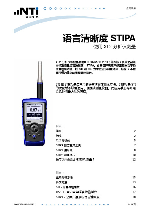
XL2-STIPA-新功能

合集下载

PCS-9691-CN_X_说明书_南瑞继保备自投

特别注意，一些通用的工作于高压带电设备的工作规则必须遵守。如果不遵守可能导致严重的人身伤亡或设备损坏。
危险！
在一次系统带电运行时，绝对不允许将与装置连接的电流互感器二次开路。该回路开路可能会产生极端危险的高压。
警告！
曝露端子在装置带电时不要触碰曝露的端子等，因为可能会产生危险的高电压。
残余电压在装置电源关闭后，直流回路中仍然可能存在危险的电压。这些电压需在数秒钟后才会消失。
本手册中将会用到以下指示标记和标准定义：
危险! 意味着如果安全预防措施被忽视，则会导致人员死亡，严重的人身伤害，或严重的设备损坏。
警告! 意味着如果安全预防措施被忽视，则可能导致人员死亡，严重的人身伤害，或严重的设备损坏。
警示! 意味着如果安全预防措施被忽视，则可能导致轻微的人身伤害或设备损坏。本条特别适用于对装置的损坏及可能对被保护设备的损坏。
P/N：ZL_PCS-9691-CN_X_说明书_国内中文_国内标准版_X
购买产品，请联系：电话：025-87178911 传真：025-52100511、025-52100512
版本：R1.01
ii
南
前言.................................................................................................................................................... i 目录.................................................................................................................................................. iii 第 1 章概述...................................................................................................................................... 1

FlexiForce标准型号A201传感器说明书

DS Rev I 062821ISO 9001:2008 Compliant & 13485:2016 RegisteredThe FlexiForce A201 is our standard sensor and meets the requirements of most customers. The A201 is a thin and flexible piezoresistive force sensor that is available off-the-shelf in a variety of lengths for easy proof of concept. These ultra-thin sensors are ideal for non-intrusive force and pressure measurement in a variety of applications. The A201 can be used with our test & measurement, prototyping, and embedding electronics, including the FlexiForce Sensor Characterization Kit, FlexiForcePrototyping Kit, FlexiForce Quickstart Board, and the ELF™ System*. You can also use your own electronics, or multimeter.FlexiForce™Standard Model A201BenefitsPhysical PropertiesThickness 0.203 mm (0.008 in.)Length 191 mm (7.5 in.)** (optional trimmed lengths: 152 mm (6 in.), 102 mm (4 in.), 51 mm (2 in.))Width14 mm (0.55 in.)Sensing Area 9.53 mm (0.375 in.) diameterConnector3-pin Male Square Pin (center pin is inactive)Substrate Polyester Pin Spacing 2.54 mm (0.1 in.)✓ROHS COMPLIANT• Thin and flexible • E asy to use• C onvenient and affordable* Sensor will require an adapter/extender to connect to the ELF System. Contact yourTekscan representative for assistance.** Length does not include pins. Please add approximately 6 mm (0.25 in.) for pin length for a total length of approximately 197 mm (7.75 in).Typical PerformanceEvaluation ConditionsLinearity (Error)< ±3% of full scaleLine drawn from 0 to 50% loadRepeatability < ±2.5%Conditioned sensor, 80% of full force applied Hysteresis < 4.5% of full scaleConditioned sensor, 80% of full force appliedDrift< 5% per logarithmic time scaleConstant load of 111 N (25 lb)Response Time < 5µsecImpact load, output recorded on oscilloscope Operating Temperature -40°C - 60°C (-40°F - 140°F)Convection and conduction heat sources Durability≥ 3 million actuations Perpendicular load, room temperature, 22 N (5 lb)Temperature Sensitivity0.36%/°C (± 0.2%/°F)Conductive heating***All data above was collected utilizing an Op Amp Circuit (shown on the next page). If your application cannot allow an Op Amp Circuit, visit/flexiforce-integration-guides, or contact a FlexiForce Applications Engineer.***©Tekscan Inc., 2021. All rights reserved. Tekscan, the Tekscan logo, and FlexiForce are trademarks or registered trademarks of Tekscan, Inc.+1.617.464.4283|1.800.248.3669|****************|/flexiforceP urchase T oday o nline aT www .Tekscan .com /sToreVOLUMEDISCOUNTSA s k U sAb o u t Ou rSensing Area14 mm (.55 in.)191 mm (7.5 in.)6 mm (.25 in.)Actual size of sensorTrim LinesV OUT = -V REF * (R F / R S )• Polarity of V REF must be opposite the polarity of V SUPPLY • Sensor Resistance R S at no load is typically >1MΩ• Max recommended current is 2.5mAV OUTC 1R F V SS = GroundV DD = V SUPPLYC 1 = 47 pFR FEEDBACK (R F ) = 100kΩ POTENTIOMETER V REF OptionsSquare Wave Up to 5V , 50% Max Duty CycleDC0.25V - 1.25VMCP6004-V REF100K potentiometer and 47 pF are general recommendations; your specific sensor may be best suited with a different potentiometer andcapacitor. Testing should be performed to determine this.R SRecommended Circuit†This sensor can measure up to 4,448 N (1,000 lb). In order to measure higher forces, apply a lower drive voltage (-0.5 V, -0.25 V, etc.) and reduce the resistance of the feedback resistor (1kΩ min.). To measure lower forces, apply a higher drive voltage and increase the resistance of the feedback resistor.Sensor output is a function of many variables, including interface materials.Therefore, Tekscan recommends the user calibrate each sensor for the application.Standard Force Rangesas Tested with Circuit Shown4.4 N (0 - 1 lb)111 N (0 - 25 lb) 445 N (0 - 100 lb) †。

SYSTIMAX GigaSPEED X10D HGS620 屏蔽式接头终端说明书

SYSTIMAX ® Solutions Instruction Sheet 860524180Issue 5, January 2013HGS620 Shielded Outlet Termination Instructions© 2013 CommScope, Inc. All rights reservedPage 1 of 6GeneralThese instructions provide the recommended termination procedure for SYSTIMAX ®GigaSPEED ®X10D HGS620 shielded outlets on F/UTP and S/FTP cables. The outlets are UL approved.Refer to the SYSTIMAX GigaSPEED X10D High Density Shielded Solutions Design and Installation Guidelines for further information.The SYSTIMAX seating tool (760152876) is required for outlet termination. Ordering information is listed below:Material ID Part No.Description760152801 HGS620HGS620 GigaSPEED X10D shielded outlet760152819HGS620-BULK100HGS620 GigaSPEED X10D shielded outlet (100 pack)How to Contact Us• To find out more about CommScope ®products, visit us on the web at / •For technical assistance:-Within the United States, contact your local account representative or technical support at 1-800-344-0223. Outside the United States, contact your local account representative or Authorized Business Partner.-Within the United States, report any missing/damaged parts or any other issues to CommScope Customer Claims at 1-866-539-2795. Outside the United States, contact your local account representative or Authorized Business Partner.Tools Required• Cable jacket scoring tool (such as Xcelite ®2CSKY or JOKARI ®No.1-Cat) • Scissors • Side cutters•SYSTIMAX seating tool.860524180Instruction SheetPage 2 of 6Preparation of F/UTP Cable for Termination1.scoring tool that has fine adjustment settings, such as the Xcelite JOKARI No.1-Cat.2. jacket.3. Trim off clear cellophane wrapping.4. Separate the pairs, cut the flute flush with endof jacket and restore pairs to their original positions. 5. Ensure that foil is pressed tight over thejacket and then wrap drain wire around foil close to end of cable. Do not overlap drain wire when wrapping. 6. Arrange pairs in the order below:• Brown • Blue • Orange • GreenPreparation of S/FTP Cable for Termination1.scoring tool that has fine adjustment settings, such as the Xcelite JOKARI No.1-Cat.2.over cable jacket.Brown pair860524180Issue 5, January 2013Page 3 of 61. termination manager with pair colors oriented to the labels on the termination manager.Important:cable or braided shield on S/FTP cable will manager.2. engage and a click is heard.Note: F/UTP cable shown.Score foil shield1” (25mm)Braided shieldDrain wire860524180Instruction SheetPage 4 of 6Seat and Trim Conductors1. Following the label colors (T568B shown),place conductors directly into termination slots. Seat conductors by pulling tight into slots, then trim pairs flush.Seat Termination Manager on Outlet Body1. Carefully align and insert terminationmanager squarely into outlet body.Note : For correct orientation, the Brown label side faces the 3 notches.2. If outlet will be used in a Keystone compatibleopening, insert Keystone clip on outlet before placing it in seating tool and seating termination manager to outlet body.Note: The clip has three tabs that slide into three notches on outlet body.Orange pairGreen pair860524180Issue 5, January 2013Page 5 of 6For F/UTP cable only, trim excess foil.6. If outlet will be used in a faceplate or boxapplication, attach M-series adapter.Note : The M-series adapter is not allowed where grounding is required.Foil860524180Instruction SheetPage 6 of 6Inspection or Repair of TerminationNote: To enable inspection or repair, the termination manager can be released from the outlet body by inserting a small flat blade screwdriver in slot located on either side of outlet and twisting as shown.To release the termination manager, insert a small flat blade screwdriver between the two halves as shown and twist to disengage the latches.A spudger tool can then be used to remove conductors for repair.Installation in Shallow BoxesIt is acceptable to bend the exiting cable up to 90°, as tight as necessary, in any direction. Use care to ensure the cable shield remains inside the termination manager.Slot。

Genie DPL Super Series 操作手册说明书

“Super Series ”是 Terex South Dakota 的商标。

符合 EC 指令 2006/42/EC请参阅 EC 符合性声明采用可回收纸印刷 L 美国印刷要点操作机器前，应阅读、理解并遵守这些安全规则和操作说明。

只有训练有素且经过授权的人员方可操作该机器。

应将此手册当作机器的一部分并始终与机器放在一起。

如果有任何问题，请与 Genie 电话联系。

目录页码安全规则 ......................................................................1控制器 ..........................................................................7图例 .............................................................................8操作前检查 ...................................................................9维护 ...........................................................................11功能测试 ....................................................................14工作场所检查 .............................................................17操作说明 ....................................................................18蓄电池和充电器说明 ..................................................21运输和提升说明 .........................................................22标贴 ...........................................................................24规格 .. (28)请与我们联系：网址：电子邮件：*********************操作手册第五版•第二次印刷安全规则危险不遵守本手册中的说明和安全规则将导致死亡和严重伤害事件的发生。

Xrite-DTP70和Epson XL 10000XL扫描仪的使用说明说明书

How to use Xrite and Epson ScannerByungseok MinMehul JainElectronic Imaging Systems LaboratorySchool of Electrical EngineeringPurdue UniversityTable of ContentPg. No.Overview 3Chapter 1: Managing X-rite1.1 Software Location 51.2 Designing Test Patterns 5 - 10 1.3 Modifying Test Patterns 11 - 13 1.4 Measuring Test Patterns 14 – 15 1.5 Exercise examples 16 - 18Chapter 2: Managing Scanner2.1 Scanner Details 192.2 Screenshots 20 - 25 2.3 Scanning Procedure 26 - 28OverviewScanner calibration is the process to estimate CIE XYZ values of the printed image from the device dependent RGB values of the scanned image.Spectro-photometer and scanner are used to obtain CIE XYZ value and to scan the image. It is essential to know how to use the devices to obtain correct data.This manual consists as follows.First, it will describe how to use Xrite-DTP70 to measure CIE XYZ values of hardcopy. And then it will describe how to use Epson XL 10000XL scanner with the option we have to choose.The other parts consist of gray balancing and regression model to explain the analytical scanner calibration model.CHAPTER 1 Managing X-rite1.1 Software LocationThe software used to manage X-rite is ‘Colorport 1.0.1’ and can be found in‘C:\Program Files\X-Rite\ColorPort\ColorPort’1.2 Designing Test Patterns in Colorport:Though the X-rite comes with a variety of test patterns, it might be best to design a different one for application in research work. Following steps should be followed while designing a test pattern.unch X-rite by running ‘C:\Program Files\X-rite\ColorPort\ColorPort’2.Select X-Rite DTP 70 from the ‘Measurement Device’ menu. Select CMYKin the color space and select the appropriate paper size and format.Figure 1 shows a screenshot of the application with the above mentionedsettings selected.Figure 1 : Screenshot showing initial settings.3. Select ‘New’ from the Patch Set menu. A window opens up as shown in Figure2.Figure 2 : Screenshot showing window that opens up after New is selected.4. Press ‘+’ sign repeatedly to get desired number of patches. A CMYK value can be given to each of the patches individually, this is optional. If left blank, a value of zero is assumed automatically. Give a name with which the pattern should be saved. Click on ‘Save’ once done with adding patches. Figure 3 shows a screen shot of ‘Customize’ window with 100 patches.5. Once ‘Save’ is pressed, the customization window disappears and the original window shows a preview of how the test pattern looks like. As mentioned earlier, the color of patches is irrelevant and only helps in depicting the visualization of test pattern. To make the designed test pattern match the requirements a few specifications can be customized.6. Click on ‘Properties’ button placed below ‘Measurement Device’. A window opens up as shown in Figure 4. ‘Patch Width’ and ‘Patch Height’ can be altered from 6 mm to 20 mm. These values can be changed to accommodate more or less test patches in a row. The header and trailer length can be altered toincrease/decrease the distance between the test patches and top and bottom red line. Figure 3 : Screenshot showing customization window7. Selecting ‘OK’ closes the properties window and updates the preview window with the change in settings.8. Click on ‘Margins’ in next to the ‘Paper Size’ section in the main window tochange the page margins. This will again give the freedom to increase / decrease the number of test patches in one row. Also, either of ‘Portrait’ and ‘Landscape’ formats can be selected to meet the requirements for the test patch.9. Test patches can be added/ deleted/modified anytime by clicking on ‘Customize’ under the ‘Patch Set’ column.Figure 4 : Screenshot showing Properties window10. Once satisfied with the test pattern, click on ‘Save Target’ and save it as a tiff file in a preferred location.11. There are further possibilities of fine tuning the test pattern. See the next section for more details.Figure 5 shows a test pattern designed using Colorport software.Figure 5: Test Pattern designed using ColorportIt should be noted that the black patches in the first and the last column represent a grid which X-rite uses to approximate the start and the end point. The test pattern above has 12 rows and 28 columns that makes the total number of test patches to be 336.When a test pattern is created using Colorport, several files are generated. One is ‘.tif’ file which is an image representation of the test pattern designed. A ‘.xml’ file is generated which contains all the information about the designed test pattern and can be used for importing and exporting test patterns. ‘.tab’ file is also generated and it contains information about the individual test patches in a test pattern. This file can be used to modify the total number of test patches etc.1.3 Modifying Existing Test Patterns:If a test pattern already exists, it can be modified in two different ways depending on the format of the file of the test pattern.1.3.1 .xml fileIf the test pattern exists in form of a .xml file, then changes can be made to the xml file to meet the requirements. The .xml file contains detailed information about specifications of the test patterns that would be used by X-rite formeasurement purposes. Figure 6 shows a sample .xml file for one of the testpatterns created using Colorport.Figure 6: screenshot showing sample .xml fileAs is clear from Figure 6 above, the .xml file contains information such as patch width, height, page width and height, page margins, etc. These values can be changed individually to meet the requirements. Unfortunately, there is no method of viewing the effects of changes made to .xml file. So, a trial and error method needs to be adopted to make the .xml file work for the test patterns in hand. Once the changes have been made, the file should be saved againas .xml file and imported into Colorport. Steps to Import the file are listed below.Importing/Exporting .xml fileFrom the file menu in Colorport, select ‘Target Manager’. A window opens up as shown in Figure 7. Click on ‘import’ and then give the location of .xml file. Same procedure can be followed for exporting a .xml file.Figure 7: screenshot showing ‘Target Manager’ window1.3.2 .tab file.tab file can be used to import individual test patches within a test pattern to create a new test pattern. To import test patches from a .tab file, follow the following steps:1. Open the .tab file in notepad and save it in .txt format.2. Make sure that the correct color space ( RGB / CMYK etc.) is selected in the menu under ‘Color Space’ column.3. Select ‘New’ from the menu in ‘Patch Set’ column.4. Click on ‘Import Patches’ button in the window that opens up. Figure 8 shows the results of importing test patches.Figure 8: screenshot showing import of test patches from .tab file5. Once the patches have been imported, relevant steps mentioned in section 1.2 can be followed to modify the test pattern as needed.1.4 Measuring Test PatternsOnce the test pattern has been created / modified using any of the steps mentioned in the previous sections, it is ready to be measured with X-rite.1. Click on the ‘Measure Target’ tab in the main window of Colorport software.2. Select X-Rite DTP 70 from the drop down menu under ‘Measurement Device’ and click on connect.3. Select the target that is to be measured in the ‘Target’ column. If the name is not listed in the menu then follow the steps mentioned for importing .xml file in section 1.3.1. Figure 9 shows a screenshot showing the ‘Measure Target’ window with appropriate settings.Figure 9: screenshot showing the measure target window.4. The right half of the window shows preview of the patches to be measured. ‘Measurement Status’ column in the lower left section of the window displays the progress of the current measurement cycle.5. Insert the printout of test pattern in X-rite and hit the orange button on the left side of X-rite. The X-rite then takes measurements6. Once the X-rite has taken measurements, click on the ‘Save Data’ button andchoose the settings in the window that comes up as shown in Figure 10 below.7. Click on ‘Continue’ button and provide a location and name to save the data file.The data file can be opened up in notepad. The data file has three columns and each row corresponds to a patch in the test pattern. For example, if there are 100 patches in the pattern, there will be 100 rows. First row in the date file corresponds to XYZ values of first patch in the first row of test pattern. Second row corresponds to second patch in the first row of the test pattern and so on. Figure 10: screenshot showing the Save Data window.1.5 Exercise examples1.5.1 Q60 measurementKodak Q60 is most common patch to be used for scanner calibration. Figure 11 shows a sample Q60 patch.Figure 11: Sample Q60 patchIn particular, the gray-levels in the bottom part of the Q60 patch are used for gray balancing. Following steps describe the procedure to be carried out for measuring all the color in Q60.1. Measure the width and height of the small square size and the gray boundaries very carefully. Any small error in measurement will bring out critical failure to obtain correct CIE XYZ values of Q60, since the aperture will measure wrong place.2. Based on the measured values, divide the whole patch including boundaries into the set of small squares. The boundary may have the same width as the small square. After all, you should be able to design .tab profile for Q60 and TIFF file that can print out the set of those squares.3. Develop a test profile in Colorport to measure Q60 by Xrite DTP70. The first step will be to develop a profile by Colorport with 18 row and 26 columns of test patches (You will see why it is 18x26). Be sure the width, height, margin and so on.4. After making the profile, the Colorport will produce a TIFF file. Print out the TIFF file, and locate the Q60 on the printed image so that you measure Q60 as if it were the printed image.5. Take the measurements using X-rite and the design developed in Step 3.1.5.2 Cyan patch for scanner calibration1. Determine the size of the patch you want to create.2. Determine the number of small squares with its height and width so that the sum of the length of the square is same as the patch size.3. Develop a profile in Colorport to measure those squares, then you willhave .tab file and tif file.4. Generated tif file will have black reference marks in both left and right side of the patch. Since you are not able to have a color of the patch, you have to refill the color by creating the same tif image by MATLAB or C.By writing your own code, you will have the tif file with the same size, but can fill the color as you want. Please be sure that your new tif file has the black reference marks too. The sample tif file is shown in figure 12.5. Print out the new tif file, and measure by Xrite.Figure 12: Sample tif fileCHAPTER 2 Managing Scanner2.1 Scanner detailsThe scanner being calibrated is Epson Expression 10000XL. The software used for scanning is VueScan (version : 8.1.28).2.2 ScreenshotsThis section presents screenshots of the settings to be used while calibrating the scanner. It is imperative that the same settings be used for measurement purposes. The choices in settings have been explained wherever necessary.2.2.1 Input TabThe settings shown in Figure 11 below are for use with Auto Document Feeder. It is important to set the bits per pixel to 24 bit RGB and Scan resolution to 600 dpi.Figure 13: screenshot of Vuescan’s ‘Input’ Tab2.2.2 Crop TabFigure 14: screenshot of Vuescan’s ‘Crop’ TabIt should be noted that most of the values will be different depending on the test pattern being scanned. For more info please see section number 2.3.1The values in ‘Border %’ , ‘Buffer %’, ‘X images’, ‘Y images’ and ‘Lock aspect ratio’ should be used as it is for the scanner settings.2.2.3Filter TabFigure 15: screenshot of Vuescan’s ‘Filter’ TabUnder the filter tab, set all the values as shown above. The values are chosen in such manner so as to minimize the software’s modifications in the actual measurements.Figure 16: screenshot of Vuescan’s ‘Color’ TabAll of the values shown in Figure 16 above should be carefully used as it is, while configuring the software.There are a variety of options present under ‘Color balance’ menu such as manual, neutral, tungsten etc. It was found out that ‘None’ works the best for calibration and measurement purposes.Selecting the correct color spaces is crucial too, and an incorrect choice might significantly alter the RGB measurements.Figure 17: screenshot of Vuescan’s ‘Output’ TabThe output files should be saved in ‘.tif’ format with ‘compression off’ and the tiff file type should be 24 bit RGB.2.2.6 Preferences TabAll the values shown in Figure 18 can be changed as per convenience and need. Figure 18: screenshot of Vuescan’s ‘Preferences’ Tab2.3 Scanning ProcedureOnce the values discussed in section 2.2 have been entered into Vuescan, it needs to be configured for scanning a particular area of the test pattern. The procedure is discussed in the next section.2.3.1 Previewing the scan area:1. Slide the paper into the auto document feeder(ADF) of the scanner.2. Click on the ‘Crop’ tab in the Vuescan software window and make sure‘Preview area’ has been set to maximum.3. An extra sheet of paper must be put below the test pattern being previewed. Skipping this step would result in an error.4. Click on ‘Preview’ button on bottom left of the screen. The ADF then feeds the test pattern and the extra sheet of paper in to the scanner. Figure 19 on the next page displays a snapshot of the preview screen.5. Select the crop area by adjusting the dotted lines. The image can be rotated by clicking on the input tab and then making changes in the ‘rotation’ menu.6. Once satisfied with the crop area and other settings, go to File menu and save the settings by selecting ‘Save options’. The settings file is saved as a ‘.ini’ file.7. After saving the file, close the Vuescan software, remove the last sheet of paper from the scanner and re-open the Vuescan software.The test patterns are now ready to be scanned. Figure 19: screenshot of Vuescan’s Preview window2.3.2 Scanning the Test Patterns1. Slide the stack of papers into the auto document feeder(ADF) of the scanner.2. Insert an extra sheet of paper in the end. This step is important, if not followed it would result in last test pattern not being scanned.3. In the Vuescan software, go to file menu and select ‘load options’. Load the ‘.ini’ file that was saved while setting the crop area ( see section 2.3.1).4. Set the appropriate output file name by going to output tab in the software window. Inserting a ‘number+’ symbol with the name starts the file name from that number and increments the number each time by 1. For example, specifying the file name as ‘magenta1+.tif’ would save the first file as ‘magenta1.tif’ the second file as ‘magenta2.tif’ and so on.5. After the scanner has finished scanning, the files can be accessed and are ready to be used.CHAPTER 3 Gray Balancing3.1 IntroductionGray balancing is a process by which a power curve relationship is developed between measured luminance (Y) and RGB values for a monochrome test pattern. The Power curve is used to convert RGB values to linearized RGB values.3.2 Procedure3.2.1 Data AcquisitionFor gray balancing purposes, it is recommended that a Q60 patch be used. It is an industrial standard and is used in wide variety of applications. Figure 18 shows a sample Q60 patch.Figure 18: Sample Q60 patchThe gray-levels in the bottom part of the Q60 patch should be used for gray balancing.Following steps describe the procedure to be carried out for gray balancing.1. Develop a test pattern in Colorport which will measure the gray patches in the Q60 test pattern. Since, Q60 is a lot different from standard test patterns measured by X-rite, a quick solution might be to develop a test pattern in Colorport with 1 row and 25 columns of test patches. The patch width, height and page margins should be carefully adjusted to match the requirements. This pattern then can be used as a guiding outline for measuring the gray patches in Q60. For more information on how to design a test pattern in Colorport, please refer to section 1.2.2. Take the measurements using X-rite and the design developed in Step 1.3. Scan the Q60 patch using Epson 10000XL scanner. Crop the scanned image to retain only the gray test patches. Figure 19 shows an image of the scanned Q60 patch.Figure 19: Scanned Q60 patch3.2.2 CalculationNow that the data has been acquired, a power curve relationship needs to be developed between the measured luminance and measured RGB values.1. Scale the measured RGB data by dividing it with 255 so that the data ranges from 0 to 1.2. Scale the measured Y values by a factor of (255/100).3. Use the inbuilt Matlab tool ‘cftool’ to fit a power curve. Figure 20 shows a snapshot of cftool.Figure 20: cftool window in Matlab.4. Click on ‘Data’ button and assign the scaled R values to x axis and scaled Y values to y axis.5. Click on the ‘Fitting’ button and in the window that opens up, choose ‘Power’ for the type of fit and choose ‘a*x^b +c’ in the section right below the type of fit column. Figure 21 shows a snapshot of settings to be chosen.Figure 21: Fitting window in cftool ( Matlab)6. Click on Apply to fit the curve. The Results section shows the equation of the fitted power curve and the associated rmsE value. This value should be as low as possible.7. Repeat steps 4,5 and 6 for green and blue components of the measured data and find the power curve equations that are the best fit for the data.This concludes the process of gray balancing . The equations developed in this section will be used in the next step called ‘ Matrix Transformation’.Figure 22 shows a plot of the gray balancing curves developed for a test case.Figure 21: Gray balancing curvesCHAPTER 4 Matrix Transformations4.1 IntroductionMatrix Transformation is a method of finding a 3 X 3 matrix for each of the color channels (Cyan, Magenta and Yellow). Data is first converted to linearized RGB using the gray balancing technique described in Chapter 3. Matrix is thencalculated by using functions in Matlab to divide the LRGB values by measured XYZ values.4.2 Procedure1. Generate a set of test patterns consisting of patterns for different gray levels for a single color channel. The set should contain sufficient number of patterns varying from lightest to darkest gray level for that color channel. This can be done using Matlab or C. Figure 22 shows test patterns that were used forcalibrating Epson 10000 XL2. Create the pattern in Colorport that will measure the generated test patterns.3. Measure the test patterns using X-rite and save all the data files. Figure 22: Test Pattern generated for matrix transformation4. Scan all the test patterns and extract the RGB values using Matlab or equivalent.5. For the measured RGB values, use the power curves calculated during Gray Balancing ( see chapter 3) to calculate the corresponding linearized RGB values.6. Once the LRGB values have been calculated, use ‘\’ ( left matrix divide operator) to divide the LRGB values with the measured XYZ values.7. The operation in Step 6 results in a 3 x 3 matrix which is the transformation matrix for that color channel.8. Now that the matrix has been calculated, it is important to check the validity of results.9. For this, generate a separate set of test patterns for that color channel and scan them to find out the RGB values.10. Convert the measured RGB values to LRGB values and use the 3x3 matrix calculated in step 7 to estimate the XYZ values.11. Find out the error between the estimated and actual XYZ values by first converting these values to LAB format and then calculating the deltaE.12. The deltaE value should be as small as possible. Typically it should be less than 0.513. Repeat steps 1 – 12 for the remaining two color channels.The 3x3 matrices have now been calculated and this concludes the process of scanner calibration.。

扩声系统安装调试

扩声系统调试本文档提供如何使用NTi Audio 设备进行扩声系统和疏散逃生系统的调试和服务。

您需要：Exel 声学套件• XL2 分析仪• M4260 量测麦克风• MR-PRO 信号发生器• ASD 缆线• 缆线测试插头• 主电源适配器• 系统工具箱TalkBox 声学信号发生器您可以：NTi Audio 仪器可用于下列测试：• 缆线测试• 测量 THD+N • 100V 阻抗测试 • 极性测试• RTA 实时频谱分析• 扬声器延迟设置• 噪声曲线• 混响时间 RT60• 语言清晰度 STIPA扩声系统安装声学套件TalkBox 声学信号发生器怎样测试缆线可以查出平衡XLR 线的任何缺陷，即便缆线已经被装到天花板，墙壁或地板内。

将缆线测试适配器连接到缆线的公头将MR-PRO信号发生器连接到缆线母头在MR-PRO 上，从菜单中选择CABLETEST 缆线测试会有醒目的提示信息显示缆线是否完好检测到断开线路缆线中两条线路连接错误，如PIN 1 和 PIN 2查错提示，请看附录 A怎样测量THD+N您系统中的某个组件可能会在信号通道中增加非预期的谐波，失真或噪声，也可能该组件没有正确安装或接地，增益过小或过大，又或者组件损坏或有质量问题。

您都可以用XL2 的THD+N功能测量总谐波失真和噪声。

将XL2 连接到系统输出端将MR-PRO 连接到系统输入端在M R-PRO 上，从主菜单选择GENERATOR 信号发生功能，选择WAV 中的SINE 正弦信号，将电平设置为0.00dBu，频率设置为1.000kHz。

在XL2 上，从主菜单选择RMS/THD+N 功能，选择零计权滤波器（测量所有频点的平坦响应），设置LVLRMS单位为dBu，THDN单位为%.显示输入信号是否平衡。

LVLRMS 值显示原始信号的增益或损失：0.0dBu 表示没有增益会损耗。

FREQ 值显示XL2 探测到的频率。

如1.00000 kHz.THDN 值是一个比率，表示XL2 收到的信号中有多少不是来自这1kHz 的正弦信号。

语言清晰度STIPA的测量

ቤተ መጻሕፍቲ ባይዱ级别 A+ A
B
C D E F
G
H
I J U
STI 范围 > 0.76 0.72 - 0.76
典型应用录音室剧院，演讲厅，议会，法院
0.68 - 0.72
剧院，演讲厅，议会，法院
0.64 - 0.68 0.60 - 0.64 0.56 - 0.60 0.52 - 0.56
电话会议，剧院教室，音乐厅
6
STIPA File Multiple_STIPA_000 (MyLocation, 6)
Noise File
[STI] 0.55
F
[STI] 0.80 A+
[STI] 0.94 A+
[STI] 0.97 A+
[STI] 0.98 A+
[STI] 0.97 A+
所有注册用户都可以在 XL2 支持页面下载 STIPA 报告生成工具（打开文件后请启用所有宏）。系统要求： • 运行 Windows XP 或 Windows 7 的计算机 • Excel 2007 或 Excel 2010 (32 位或 64 位版本)
标准
ISO 7240-16 / - 19 标准要求验证电声音响系统紧急用途：根据实际情况确定最低水平的语言清晰度，以防遇到紧急情况。因而，严格监管下的语言清晰度不是一个主观测量，而是必须是经过验证的、多少有些复杂的方法，这些测量方法在 IEC 60268-16 中已经被标准化。
国际标准： ISO 7240 IEC 60268-16
3 / 19 页

应用手册
• 心里声学效果（掩蔽效应）
人耳听觉系统在声压级较低或者较高的时候，敏感度降低：声压级较低时（例如20-50dBSPL)，由于听觉阈值作用而导致人耳敏感度降低。当声压级较高时（例如大于80dBSPL)，掩蔽效应导致人耳敏感度降低。

3D打印机uprint说明书

.
目录
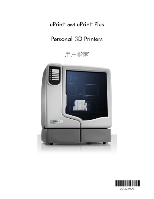
简介
指南使用说明................................................................................................................................................................ 1 了解更多信息！ ........................................................................................................................................................... 1 安全防范措施............................................................................................................................................................... 2
将打印机联网............................................................................................................................................................... 9 通过网络进行连接：......................................................................................................................................... 9 直接连接到工作站上：..................................................................................................................................... 9

1、下载文档前请自行甄别文档内容的完整性，平台不提供额外的编辑、内容补充、找答案等附加服务。
2、"仅部分预览"的文档,不可在线预览部分如存在完整性等问题,可反馈申请退款(可完整预览的文档不适用该条件!)。
3、如文档侵犯您的权益，请联系客服反馈,我们会尽快为您处理(人工客服工作时间：9:00-18:30)。

Key Challenge 主要挑战
Solution 解决方案
1. Record the ambient noise level 记录背景噪声平记录背景噪声电平 2. Measure STI when the place is deserted 测量安静条件下STI值 3. Mix the two data to g get the correct STI result 整合两组数据以得到正确的STI结果
Distortions 失真
SPL Frequency response 声压级频率响应
New Workflow 新测量流程
The new XL2 firmware offers an efficient workflow to measure STI and to optimize the PA system
XL2 measures noise, then STI
•
Test requirements 测量要求
STI measurement time 15 sec.
STI测试时间为15秒典型值： STI>0.6
Typical requirement: STI > 0.6 06
0.6 STI (typ. limit)
• takes 15 seconds 费时 15秒 • requires a special test signal 播放特定的测试信号 • must be repeated every 6 m 每6米间隔需重复测试 • is i affected ff t d by b human h noise i 受人群噪声影响
• Covered topics 涵盖主题
1. 2 2. 3. 4. 5. New STIPA measurement workflow of XL2 FW v2.50 XL2固件 V2.50中 STIPA测量 Practical presentation 实际演示 New edition of STIPA standard, best practices STIPA 新标准最佳范例 STIPA新标准，最佳范例 New reporting tool 新报告生成工具 Q&A, auxiliary information 问和答，其他信息
Reporting Tool
报告生成工具
• Import p the saved STIPA file with embedded noise data into the Excel template 将含环境噪声数据将包含环境噪声数据的 STIPA数据存储文件导入 Excel模板文件中 • Check the correctness of the acquired data 检查数据的正确性 • Add or remove data sets 添加或移除数据 • Print out the report sheet 打印报告文件
A+
A
0.74
B
0.7
Hi h speech High h intelligibility i t lli ibilit 高语言清晰度
C
0 66 0.66
High g speech p intelligibility g y 高语言清晰度
D
0.62
Good speech intelligibility 较好的语言清晰度
STIPA 测量范例 STIPA测量范例
NTi Audio has compiled a doc with information on how to measure STIPA in practice. NTi Audio 将如何在实际应用中测量 STIPA的相关信息整合在了文档中 Visit our website 访问官网 www.nti‐ to learn more or download our application li i note on Installed I ll d Sound, S d Evacuation Systems 学习或下载更多关于现场音频系统或疏疏散系统的应用手册统
F
0.54
Good quality PA systems 较好的扩声系统
G
0.5
Target value for VA systems 适用语音报警系统
H
0.46
Normal lower limit for VA systems 低标准语音报警系统
I
0.42
J U
0.38 < 0.36பைடு நூலகம்
STIPA Good Practices
Conclusion
结论
Questions welcome! 欢迎大家的提问！
Webinar download 网络研讨会下载: http://my.nti‐/partner/presentations.php
STI (be est case)
STI Qualification Bands
STI结果评估（1）
Category 级别 Nominal STI 典型值 > 0.76 Complex messages, unfamiliar words 复杂的信息，不熟悉的单词 Complex messages, f ili words d unfamiliar 复杂的信息，不熟悉的单词 Complex messages, unfamiliar words 复杂的信息，不熟悉的单词 Complex messages, familiar words 复杂的信息复杂的信息，熟悉的单词 Type of message information 信息类型 Examples of typical uses 典型应用 Recording studios 录音室 Theatres, speech auditoria, parliaments, courts, assistive hearing systems (AHS) 剧院，语音会议，国会，法院，辅助听觉系统（AHS） Theatres, speech auditoria, parliaments, courts, t assistive i ti hearing h i systems t (AHS) 剧院，语音会议，国会，法院，辅助听觉系统（AHS） Theatres, speech auditoria, parliaments, courts t 剧院，语音会议，国会，法院 Lecture theatres, classrooms, concert halls 演讲厅，教室，音乐厅 Comments 评价 Excellent intelligibility 极优异语言清晰度 High speech intelligibility 高语言清晰度
STIPA Measurement STIPA 测试
The presence of a public has a big influence on the STI results 公共环境噪声对 STI结果有很大影响
Reverberation time 混响时间
Ambient noise 环境噪声
Practical Presentation 实际演示
• Test setup 测试步骤
MR‐PRO plays ambient noise, then STIPA test signal via loudspeaker
MR-PRO播放环境噪声，并通过扬声器播放STIPA 测试信号 XL2测量噪声，然后测量STI
STI Qualification Bands STI结果评估（2）
E 0.58 Complex messages, familiar context 复杂的信息复杂的信息，熟悉的单词 Complex messages, familiar context 复杂的信息，熟悉的单词 Complex messages, familiar context 复杂的信息，熟悉的单词 Simple messages, familiar words 简单的信息，熟悉的单词 Simple messages, familiar context 简单的信息，熟悉的单词 Concert halls, modern churches 音乐厅现代化教堂音乐厅，现代化教堂 PA systems in shopping malls, public building offices, cathedrals 商场的扩声系统，公共办公区域，教堂 Shopping malls, public building offices, VA (voice alarm) systems 商场，公共办公区域，语音报警系统 VA and PA systems in difficult acoustic environments 困难声学环境下的语音与扩声系统 VA and PA systems in very difficult spaces 恶劣环境下的语音与扩声系统 Not suitable for PA systems 不适用于扩声系统 Not suitable for PA systems 不适用于扩声系统 High quality PA systems 高质量扩声系统
Key Challenge 主要挑战
Mission 任务
Evaluate the STIPA speech intelligibility in a public place 评估公共场合语言清晰度 STIPA
Challenge 挑战
Each STI measurement 每次 STI测量 STI 测量
优化扩声系统以获得较好的STI结果
Ambient noise (as in case of emergency) 环境噪声（譬如紧急情况下）
On‐board processing of noise & STIPA data adjust the PA‐ system 仪器内部直接处理环境噪声与STI数据调试扩声系统