A precise approximation for directed percolation in d=1+1

合集下载

运筹学英汉词汇ABC

运筹学英汉词汇(0,1) normalized ――0-1规范化Aactivity ――工序additivity――可加性adjacency matrix――邻接矩阵adjacent――邻接aligned game――结盟对策analytic functional equation――分析函数方程approximation method――近似法arc ――弧artificial constraint technique ――人工约束法artificial variable――人工变量augmenting path――增广路avoid cycle method ――避圈法Bbackward algorithm――后向算法balanced transportation problem――产销平衡运输问题basic feasible solution ――基本可行解basic matrix――基阵basic solution ――基本解basic variable ――基变量basic ――基basis iteration ――换基迭代Bayes decision――贝叶斯决策big M method ――大M 法binary integer programming ――0-1整数规划binary operation――二元运算binary relation――二元关系binary tree――二元树binomial distribution――二项分布bipartite graph――二部图birth and death process――生灭过程Bland rule ――布兰德法则branch node――分支点branch――树枝bridge――桥busy period――忙期Ccapacity of system――系统容量capacity――容量Cartesian product――笛卡儿积chain――链characteristic function――特征函数chord――弦circuit――回路coalition structure――联盟结构coalition――联盟combination me――组合法complement of a graph――补图complement of a set――补集complementary of characteristic function――特征函数的互补性complementary slackness condition ――互补松弛条件complementary slackness property――互补松弛性complete bipartite graph――完全二部图complete graph――完全图completely undeterministic decision――完全不确定型决策complexity――计算复杂性congruence method――同余法connected component――连通分支connected graph――连通图connected graph――连通图constraint condition――约束条件constraint function ――约束函数constraint matrix――约束矩阵constraint method――约束法constraint ――约束continuous game――连续对策convex combination――凸组合convex polyhedron ――凸多面体convex set――凸集core――核心corner-point ――顶点（角点）cost coefficient――费用系数cost function――费用函数cost――费用criterion ; test number――检验数critical activity ――关键工序critical path method ――关键路径法（CMP ）critical path scheduling ――关键路径cross job ――交叉作业curse of dimensionality――维数灾customer resource――顾客源customer――顾客cut magnitude ――截量cut set ――截集cut vertex――割点cutting plane method ――割平面法cycle ――回路cycling ――循环Ddecision fork――决策结点decision maker决――策者decision process of unfixed step number――不定期决策过程decision process――决策过程decision space――决策空间decision variable――决策变量decision决－－策decomposition algorithm――分解算法degenerate basic feasible solution ――退化基本可行解degree――度demand――需求deterministic inventory model――确定贮存模型deterministic type decision――确定型决策diagram method ――图解法dictionary ordered method ――字典序法differential game――微分对策digraph――有向图directed graph――有向图directed tree――有向树disconnected graph――非连通图distance――距离domain――定义域dominate――优超domination of strategies――策略的优超关系domination――优超关系dominion――优超域dual graph――对偶图Dual problem――对偶问题dual simplex algorithm ――对偶单纯形算法dual simplex method――对偶单纯形法dummy activity――虚工序dynamic game――动态对策dynamic programming――动态规划Eearliest finish time――最早可能完工时间earliest start time――最早可能开工时间economic ordering quantity formula――经济定购批量公式edge ――边effective set――有效集efficient solution――有效解efficient variable――有效变量elementary circuit――初级回路elementary path――初级通路elementary ――初等的element――元素empty set――空集entering basic variable ――进基变量equally liability method――等可能性方法equilibrium point――平衡点equipment replacement problem――设备更新问题equipment replacing problem――设备更新问题equivalence relation――等价关系equivalence――等价Erlang distribution――爱尔朗分布Euler circuit――欧拉回路Euler formula――欧拉公式Euler graph――欧拉图Euler path――欧拉通路event――事项expected value criterion――期望值准则expected value of queue length――平均排队长expected value of sojourn time――平均逗留时间expected value of team length――平均队长expected value of waiting time――平均等待时间exponential distribution――指数分布external stability――外部稳定性Ffeasible basis ――可行基feasible flow――可行流feasible point――可行点feasible region ――可行域feasible set in decision space――决策空间上的可行集feasible solution――可行解final fork――结局结点final solution――最终解finite set――有限集合flow――流following activity ――紧后工序forest――森林forward algorithm――前向算法free variable ――自由变量function iterative method――函数迭代法functional basic equation――基本函数方程function――函数fundamental circuit――基本回路fundamental cut-set――基本割集fundamental system of cut-sets――基本割集系统fundamental system of cut-sets――基本回路系统Ggame phenomenon――对策现象game theory――对策论game――对策generator――生成元geometric distribution――几何分布goal programming――目标规划graph theory――图论graph――图HHamilton circuit――哈密顿回路Hamilton graph――哈密顿图Hamilton path――哈密顿通路Hasse diagram――哈斯图hitchock method ――表上作业法hybrid method――混合法Iideal point――理想点idle period――闲期implicit enumeration method――隐枚举法in equilibrium――平衡incidence matrix――关联矩阵incident――关联indegree――入度indifference curve――无差异曲线indifference surface――无差异曲面induced subgraph――导出子图infinite set――无限集合initial basic feasible solution ――初始基本可行解initial basis ――初始基input process――输入过程Integer programming ――整数规划inventory policy―v存贮策略inventory problem―v货物存储问题inverse order method――逆序解法inverse transition method――逆转换法isolated vertex――孤立点isomorphism――同构Kkernel――核knapsack problem ――背包问题Llabeling method ――标号法latest finish time――最迟必须完工时间leaf――树叶least core――最小核心least element――最小元least spanning tree――最小生成树leaving basic variable ――出基变量lexicographic order――字典序lexicographic rule――字典序lexicographically positive――按字典序正linear multiobjective programming――线性多目标规划Linear Programming Model――线性规划模型Linear Programming――线性规划local noninferior solution――局部非劣解loop method――闭回路loop――圈loop――自环（环）loss system――损失制Mmarginal rate of substitution――边际替代率Marquart decision process――马尔可夫决策过程matching problem――匹配问题matching――匹配mathematical programming――数学规划matrix form ――矩阵形式matrix game――矩阵对策maximum element――最大元maximum flow――最大流maximum matching――最大匹配middle square method――平方取中法minimal regret value method――最小后悔值法minimum-cost flow――最小费用流mixed expansion――混合扩充mixed integer programming ――混合整数规划mixed Integer programming――混合整数规划mixed Integer ――混合整数规划mixed situation――混合局势mixed strategy set――混合策略集mixed strategy――混合策略mixed system――混合制most likely estimate――最可能时间multigraph――多重图multiobjective programming――多目标规划multiobjective simplex algorithm――多目标单纯形算法multiple optimal solutions ――多个最优解multistage decision problem――多阶段决策问题multistep decision process――多阶段决策过程Nn- person cooperative game ――n人合作对策n- person noncooperative game――n人非合作对策n probability distribution of customer arrive――顾客到达的n 概率分布natural state――自然状态nature state probability――自然状态概率negative deviational variables――负偏差变量negative exponential distribution――负指数分布network――网络newsboy problem――报童问题no solutions ――无解node――节点non-aligned game――不结盟对策nonbasic variable ――非基变量nondegenerate basic feasible solution――非退化基本可行解nondominated solution――非优超解noninferior set――非劣集noninferior solution――非劣解nonnegative constrains ――非负约束non-zero-sum game――非零和对策normal distribution――正态分布northwest corner method ――西北角法n-person game――多人对策nucleolus――核仁null graph――零图Oobjective function ――目标函数objective( indicator) function――指标函数one estimate approach――三时估计法operational index――运行指标operation――运算optimal basis ――最优基optimal criterion ――最优准则optimal solution ――最优解optimal strategy――最优策略optimal value function――最优值函数optimistic coefficient method――乐观系数法optimistic estimate――最乐观时间optimistic method――乐观法optimum binary tree――最优二元树optimum service rate――最优服务率optional plan――可供选择的方案order method――顺序解法ordered forest――有序森林ordered tree――有序树outdegree――出度outweigh――胜过Ppacking problem ――装箱问题parallel job――平行作业partition problem――分解问题partition――划分path――路path――通路pay-off function――支付函数payoff matrix――支付矩阵payoff――支付pendant edge――悬挂边pendant vertex――悬挂点pessimistic estimate――最悲观时间pessimistic method――悲观法pivot number ――主元plan branch――方案分支plane graph――平面图plant location problem――工厂选址问题player――局中人Poisson distribution――泊松分布Poisson process――泊松流policy――策略polynomial algorithm――多项式算法positive deviational variables――正偏差变量posterior――后验分析potential method ――位势法preceding activity ――紧前工序prediction posterior analysis――预验分析prefix code――前级码price coefficient vector ――价格系数向量primal problem――原问题principal of duality ――对偶原理principle of optimality――最优性原理prior analysis――先验分析prisoner’s dilemma――囚徒困境probability branch――概率分支production scheduling problem――生产计划program evaluation and review technique――计划评审技术(PERT) proof――证明proper noninferior solution――真非劣解pseudo-random number――伪随机数pure integer programming ――纯整数规划pure strategy――纯策略Qqueue discipline――排队规则queue length――排队长queuing theory――排队论Rrandom number――随机数random strategy――随机策略reachability matrix――可达矩阵reachability――可达性regular graph――正则图regular point――正则点regular solution――正则解regular tree――正则树relation――关系replenish――补充resource vector ――资源向量revised simplex method――修正单纯型法risk type decision――风险型决策rooted tree――根树root――树根Ssaddle point――鞍点saturated arc ――饱和弧scheduling (sequencing) problem――排序问题screening method――舍取法sensitivity analysis ――灵敏度分析server――服务台set of admissible decisions(policies) ――允许决策集合set of admissible states――允许状态集合set theory――集合论set――集合shadow price ――影子价格shortest path problem――最短路线问题shortest path――最短路径simple circuit――简单回路simple graph――简单图simple path――简单通路Simplex method of goal programming――目标规划单纯形法Simplex method ――单纯形法Simplex tableau――单纯形表single slack time ――单时差situation――局势situation――局势slack variable ――松弛变量sojourn time――逗留时间spanning graph――支撑子图spanning tree――支撑树spanning tree――生成树stable set――稳定集stage indicator――阶段指标stage variable――阶段变量stage――阶段standard form――标准型state fork――状态结点state of system――系统状态state transition equation――状态转移方程state transition――状态转移state variable――状态变量state――状态static game――静态对策station equilibrium state――统计平衡状态stationary input――平稳输入steady state――稳态stochastic decision process――随机性决策过程stochastic inventory method――随机贮存模型stochastic simulation――随机模拟strategic equivalence――策略等价strategic variable, decision variable ――决策变量strategy (policy) ――策略strategy set――策略集strong duality property ――强对偶性strong ε-core――强ε-核心strongly connected component――强连通分支strongly connected graph――强连通图structure variable ――结构变量subgraph――子图sub-policy――子策略subset――子集subtree――子树surplus variable ――剩余变量surrogate worth trade-off method――代替价值交换法symmetry property ――对称性system reliability problem――系统可靠性问题Tteam length――队长tear cycle method――破圈法technique coefficient vector ――技术系数矩阵test number of cell ――空格检验数the branch-and-bound technique ――分支定界法the fixed-charge problem ――固定费用问题three estimate approach一―时估计法total slack time――总时差traffic intensity――服务强度transportation problem ――运输问题traveling salesman problem――旅行售货员问题tree――树trivial graph――平凡图two person finite zero-sum game二人有限零和对策two-person game――二人对策two-phase simplex method ――两阶段单纯形法Uunbalanced transportation problem ――产销不平衡运输问题unbounded ――无界undirected graph――无向图uniform distribution――均匀分布unilaterally connected component――单向连通分支unilaterally connected graph――单向连通图union of sets――并集utility function――效用函数Vvertex――顶点voting game――投票对策Wwaiting system――等待制waiting time――等待时间weak duality property ――弱对偶性weak noninferior set――弱非劣集weak noninferior solution――弱非劣解weakly connected component――弱连通分支weakly connected graph――弱连通图weighed graph ――赋权图weighted graph――带权图weighting method――加权法win expectation――收益期望值Zzero flow――零流zero-sum game――零和对策zero-sum two person infinite game――二人无限零和对策。

SR05.TCT中文资料

Forward Voltage vs. Forward Current
10 9
% Change in Capacitance 0 -2 -4 -6 -8 -10 -12 -14 -16
Capacitance vs. Reverse Voltage
Forward Voltage - V F (V)
8 7 6 5 4 3 2 1 0 0 5 10 15 20 25 30 35 40 45 50 Forward Current - IF (A) Waveform Parameters: tr = 8µs td = 20µs
SR05

Mechanical Characteristics
JEDEC SOT-143 package UL 497B listed Molding compound flammability rating: UL 94V-0 Marking : R05 Packaging : Tape and Reel per EIA 481
0
25
50
75
100
125
150
Ambient Temperature - TA (oC)
Pulse Waveform
110 100 90 80 Percent of IPP 70 60 50 40 30 20 10 0 0 5 10 15 Time (µs) 20 25 30 td = IPP/2 e
10 Peak Pulse Power - PPk (kW)
Power Derating Curve
1IP 90 80 70 60 50 40 30 20 10 0
1
0.1

Quality-driven evaluation of trigger conditions on streaming time series

Evaluating Trigger Conditions on Streaming Time Series with User-given Quality Requirements1 Like Gao2Min Wang3X.Sean Wang2 2CS Dept.,Univ.of Vermont,VT,USA.{lgao,xywang}@3IBM T.J.Watson Research Center,NY,USA.min@ Abstract:For many applications,it is important to evaluate trigger conditions on streaming time series.In a resource constrained environment,users’needs should ul-timately decide how the evaluation system balances the competing factors such as evaluation speed,result precision,and load shedding level.This paper presents a ba-sic framework for evaluation algorithms that takes user-speciﬁed quality requirements into consideration.Three optimization algorithms,each under a diﬀerent set of user-deﬁned probabilistic quality requirements,are provided in the framework:(1)minimize the response time given accuracy requirements and without load shedding;(2)min-imize the load shedding given a response time limit and accuracy requirements;and (3)minimize one type of accuracy errors given a response time limit and without load shedding.Experiments show that these optimization algorithms eﬀectively achieve their optimization goals while satisfying the corresponding quality requirements.Key Words:QoS(Quality of Service),trigger,streaming time series,prediction model Category:H.21IntroductionIn many situations an application system needs to react to preset trigger con-ditions in a timely manner.For example,in network management systems,we may want to quickly divert traﬃc from certain area once a congestion is dis-covered;in road traﬃc control,we may want to immediately enact a camera when a car crosses a certain line while the traﬃc signal is red;and in environ-mental monitoring,we may want to start taking rain samples soon after certain event happens.In this paper,we tackle this monitoring problem in which trigger conditions need to be evaluated continuously on streaming time series.Consider a stock market monitoring system where each stock s i is a streaming time series.A stock broker may register many requests for his/her clients such as “notify Alice whenever stocks s1and s2are correlated with a correlation value above0.85during a one-hour period.”The system is to monitor the streaming stock data and trigger the actions in the requests whenever the corresponding conditions are evaluated true.A perfect system would trigger the corresponding action without any delay whenever a condition becomes true.However,delay is unavoidable in a resource constrained environment.This delay can be alleviated by allowing approximateevaluation and load shedding.We here deﬁne approximate evaluation as to allow some conditions that are actually true(false)to be reported false(true,resp.), and load shedding as to selectively skip a fraction of conditions from evaluation.Approximation and load shedding may lead to errors.However,their results may still be useful.These two methods have appeared in the literature in other contexts as well,e.g.,ANN[2]is developed to searching for approximate nearest neighbors and a load shedding strategy is deployed in Aurora system[13,1,4].Approximation can be useful in at least two ways.(1)End users may be satisﬁed with approximate results,but it is important that users are given the ability to specify an error bound.(2)Or an application system may use approxi-mate results for optimization purposes.For example,a“speculative optimization strategy”can use fast approximate results to prepare(e.g.,prefetch)for subse-quent complex activities,while precise results can later be used to correct any error made in the aggressive,speculative phase[14].In this scenario,precision and response time need to be balanced in order to achieve the best overall per-formance.In this case,the application system is the“user”,and it is important that the approximate algorithms can satisfy the“user”requirements.Response time,approximation error,and load shedding level are competing factors.In this paper,we advocate that it’s the users’needs that should ulti-mately decide how the evaluation system balances them.That is,the evaluation system should satisfy user-speciﬁed quality requirements in terms of these three factors.In other words,a concept of quality of service is needed.The resulting evaluation system is called quality-driven.For a quality-driven system,it is important to have the ability to measure the(intermediate)result quality during the evaluation process.However,it is impossible to measure the accuracy(i.e.,false positive and negative ratios)pre-cisely when an approximation method is used.Indeed,the precise accuracy can only be measured a posteriori,i.e.,only after we know the actual evaluation results of the trigger conditions.Instead,we measure accuracy in an a priori manner,i.e.,the false ratios are estimated before the conditions are evaluated. To do this,we build a prediction model based on historical data analysis.At the evaluation time,we use this prediction model to derive accuracy estimates that are used to guide the evaluation.Since the evaluation procedure is based on probabilistic prediction models, our system cannot satisfy accuracy in a strict sense.Instead,we use a concept similar to the soft quality of service(QoS)in computer networks[5].That is, the system guarantees with enough conﬁdence that the expected accuracy will be more than the given thresholds.Speciﬁcally,the system allows users to impose the following quality constraints:–Response time constraint:All evaluation results must be reported within a given time limit.–Drop ratio constraint:The percentage of the conditions that are skipped(no evaluation results are reported for them)cannot exceed a given threshold.–Accuracy constraints:The expected false positive and negative ratios must not exceed the given thresholds,with enough conﬁdence(the conﬁdence is deduced from the prediction model).Ideally,users should be able to impose any combination of the above con-straints.But the evaluation system may not be able to satisfy all the constraints simultaneously.To solve this problem,one way is to ask the users to give up on some constraints(i.e.,leave as unconstrained)and let the evaluation system to do its best in terms of these constraints,while satisfying the imposed constraints on the remaining parameters.In our scenario,if one constraint is left unspeciﬁed, the system can always satisfy all other constraints.This leads to three possible choices.For each choice,we provide an evaluation algorithm in this paper.This paper makes three contributions.First,we initiate the study of a quality-driven system for evaluating trigger conditions on streaming time series.Second, we show how to use a prediction model to deduce the accuracy estimates.Third, we provide quality-driven evaluation algorithms,and show their eﬀectiveness.The rest of the paper is organized as follows.In Section2,we review re-lated work.In Section3,we formally deﬁne the trigger conditions and the qual-ity parameters.In Section4,we introduce our prediction model and deﬁne the probabilistic quality constraints.We present evaluation algorithms in Section5 and present our experimental results in Section6.We conclude the paper with discussion on future research directions in Section7.2Related WorkThe quality-driven aspect of our work is similar to the QoS concept in computer networks[8,12].This paper adopts the QoS concept into trigger condition evalu-ation on streaming time series and presents a basic design strategy for developing such a quality-driven system.Aurora[13,1,4]seems to be the only data stream processing system that contains a QoS component.In Aurora,a user may register an application with a QoS speciﬁcation.Aurora tries to maximize an overall QoS function when it makes scheduling and load-shedding decisions.In our system,we allow multiple QoS parameters,and our system optimizes an unconstrained quality parameter while satisfying users-imposed constraints on all the remaining parameters.With limited resources,using approximation techniques in processing con-tinuous queries on data streams has been studied in[7,9,6,11].However,most approximate evaluation strategies only consider one quality aspect and neglect the others.For example,Chain[3]minimizes the memory usage without consid-ering the response time at all.Our work diﬀers from all such work in that we take diﬀerent user-speciﬁed quality requirements into consideration.3PreliminaryA time series is aﬁnite sequence of real numbers and the number of values in a time series is its length.A streaming time series,denoted s,is an inﬁnite sequence of real numbers.At each time position t,however,the streaming time series takes the form of aﬁnite sequence,assuming the last real number is the one that arrived at time t.In this paper,we assume that all streams are synchronized, that is,each stream has a new value available at the same time position.In general,a trigger condition can be any user-deﬁned predicate on streaming time series,and needs to be evaluated after every data arrival.We denote a set of conditions as C={c1,c2,...,c n}and the reported evaluation result of condition c i at time position t as r(c i,t).We denote the precise evaluation result (the actual value of the given condition if a precise evaluation process is used)of c i at time position t as R(c i,t).Obviously,we have r(c i,t)∈{True,False},and R(c i,t)∈{True,False}.4Note that r(c i,t)may not be equal to R(c i,t)due to the approximate nature of the system.Let C T denote all the conditions in C whose reported results are True at time position t,i.e.,C T={c i∈C|r(c i,t)=True}. Similarly,let C F={c i∈C|r(c i,t)=False}and C D={c i∈C|c i is dropped at time position t}.We call C T,C F and C D the reported-True set,reported-False set,and dropped set,respectively.Using the above notation,we deﬁne four parameters:1.Response Time,RT,is the duration from the data arrival time t to the timewhen last condition c i,r(c i,t)=True,is reported.2.Drop Ratio,DR,is the fraction of the conditions(among all the conditionsin C)that are dropped(not reported).3.False Positive Ratio,FPR,of a reported-True set C T is the fraction of theconditions(among all the conditions in C T)whose actual values are False.We deﬁne FPR=0if C T is an empty set.4.False Negative Ratio,FNR,of a reported-False set C F is similarly deﬁned.Note that response time is deﬁned only on conditions that are reported true.4Prediction ModelWhile it is easy and straightforward to measure the quality parameters RT and DR at any time,it is diﬃcult to measure the other two parameters,FPR and FNR,without actually evaluating all the conditions.A practical solution is to build a prediction model using historical evaluation results and calculate the expected FPR and FNR based on the model in a probabilistic manner.For each condition c i,we deﬁne a random variable X i to state the outcome of its evaluation.Clearly,X i follows Bernoulli distribution X i∼B(ρi),that is,X i= 1if R(c i)=True0if R(c i)=False with P(X i=1)=ρiP(X i=0)=1−ρi.In this paper,we make the simplifying assumption that all X i’s(for1≤i≤n) are mutually independent.Clearly,the meanρi is also the expected value of X i.Depending on how the system treats c i,we see three diﬀerent cases for ρi:(1)c i is precisely evaluated.In this case,we haveρi=1if c i is evaluated to be True andρi=0if c i is evaluated to be False.(2)c i’s result is reported based on an approximation procedure,e.g.,prediction.In this case,ρi cannot be known exactly.Instead,its estimateˆρi will be used.Speciﬁcally,ˆρi can be approximated by a normal distribution function Norm(µi,σ2i),where the meanvalueµi=¯X i and the varianceσ2i=(1−µi)µiN ).(Here,¯X i denotes the sample mean,and N the sample size.)We may obtain the above by analyzing the historical evaluation results for each condition,i.e.,by adopting a data mining approach.(Examples can be found in[10,14].)(3)Too little historical data to estimateρi.For all the three cases,the estimate ofρi can be viewed as a random variable that follows normal distribution as shown below.Caseσ2i1(or0)known True or FalseµiNotherwise0.255Optimization AlgorithmsIn this section,we provide optimization algorithms for the three optimization problems mentioned in the introduction.Each problem requires a diﬀerent strat-egy.For simplicity,in all these algorithms,we assume that the precise evaluation of each condition has the same cost.Thus,the response time can be measured by the number of conditions that have been precisely evaluated (to either True or False )before the last condition in the reported-True set is reported.As mentioned earlier,the user imposes constraints on all quality parameters except for one that is left unconstrained.The evaluation system will optimize for the unconstrained parameter while satisfying the constraints on others.For the cases that the unconstrained parameter is either FPR or FNR ,we just give the algorithm for the FNR unconstrained case since the other one is symmet-ric.Thus,we study three optimization problems,namely,1)minimize response time given accuracy requirements and no drop,2)minimize drop ratio given response time and accuracy requirements,and 3)minimize false negative ratio given response time and false positive error requirements and no drop.5.1Algorithm for minimizing response timeThe algorithm is shown in Fig.1.The basic idea is to increase the size of C T and C F aggressively,and at the same time,try to report as early as possible those trigger conditions in C T .We use a greedy algorithm for this purpose.In the algorithm,we need to exam if the F P R -quality of a set C T ={c 1,...,c m }satisﬁes a given FPR -constraint τFPR (using our predicted µi values).Since we already know that the expected value of FPR follows normal distribution,we can get the conﬁdence βT with the standard normal distribution function η:βT =η(z T ),where η(x )=12π x −∞e −t 2/2dt,and z T = m i =1(θE −(1−µi )) m i =1σ2i.Note z T value can be calculated incrementally.The algorithm uses a list (called µList )that contains all the conditions in C arranged in the order,say c 1,...,c n ,such that µ1≥···≥µn .The algo-rithm starts with using InitExpandC T to get initial report-True set C T .(This InitExpandC T procedure obtains,without evaluating any conditions,an ini-tial set of conditions that can be reported true without violating the user re-quirements.)The trigger conditions in C T are reported to be True .Both the FPR -constraint τFPR and µ>0.5are satisﬁed by C T by the property of InitExpandC T .These are the trigger conditions that can be reported True with-out doing any precise evaluation.This is Step 1.After Step 1,we need to precisely evaluate trigger conditions in order to report them true (without violating either τFPR or µ>0.5).In Step 2,as a greedy algorithm,we pick up the condition having the highest µvalue.This is the one immediately after the conditions in the initial C T .Hence,we pick it (i.e.,Consts.:minimize response time(RT)Form and report the reported-True set:Init.z T=0,[z T,i T]=InitExpandC T(z T)and report c1,...,c iT−1as True.Step2.{-Precisely evaluate c iT.Two outcomes:o If c iT is evaluated True,update z T with an extra reported-True condition,[z T,∆T]=ExpandC T(z T,i T+1),and report c iT ,...,c iT+∆Tas True.Continue the loop with i T=i T+∆T+1.Form the reported-False set:Init.z F=0,[z F,i F]=InitExpandC F(z F) Step4.{-Precisely evaluate c iT.Two outcomes:o If c iT is evaluated False,update z F with an extra reported-False condi-tion,[z F,∆F]=ExpandC F(z F,i F).Update i F=i F−∆F and continuethe loop with i T=i T+1.Report as False all those conditions that were not reported True.Figure1:Algorithm MinResponse.c iT)up for precise evaluation.If the condition is evaluated True,we add it to C T and try to expand C T without precise evaluation again(by calling Procedure ExpandC T),report the conditions in the expended C T and keep going.If the condition is evaluated False,then we just keep going to precisely evaluate the next condition.During Step2,if we run out of conditions inµList,we can stop(just report all the conditions that were evaluated False as false and thus achieve FNR=0). If theµList is not exhausted,then we need to reach theﬁrst trigger condition in theµLis t such that itsµvalue is no greater than0.5.Once we only have conditions withµno greater than0.5,we need to precisely evaluate them and report them as soon as they are evaluated True.However, there is a chance we may be able to report them False.Therefore,Step3tries to get the maximum set of trigger conditions to report False without precise evaluation(note that all the conditions that were evaluated False need to be taken into account,hence the z F value may not start with0in Step3).After Step3,if we still have trigger conditions that need to be processed (i.e.,if i T≤i F),we will pick them up for evaluation.Since we want to minimize the response time for the conditions in C T,we precisely evaluate the conditions starting from those with greaterµvalues.Again,if any condition is evaluated False,we will try to expand C F.5.2Algorithm for minimizing drop ratioIn this optimization problem,we have a deadline to report all conditions in the reported-True set,which is exactly the limit on the total number of conditions that can be precisely evaluated.In addition,we still want both C T and C F to satisfy the given quality constraints(i.e.,τFPR andτFNR).In this case,we want to reduce the number of conditions that are dropped,i.e.,minimizing DR.Fig.2 shows the pseudo-code for our algorithm.Consts.:minimize drop ratio(DR)For the reported-True set C T:init.z T=0,[z T,i T]=InitExpandC T(z T).Step2.Expand C T and C F:3.1.Let z′F=z F and update z F with an extra reported-False condition,then[z F,∆F]=ExpandC F(z F,i F)3.3.{-If∆T>∆F,k=i T+∆T,else k=i F−∆F;o If c k is evaluated True,do Step3.1again,then continue the loop;}Step4.Report all conditions that were evaluated True or are in C T as True.Reportall conditions that were evaluated False or are in C F as False.The remainingconditions are dropped.Figure2:Algorithm MinDrop.The diﬀerence between this algorithm and MinResponse lies in what we em-phasize on.In MinResponse,we want to report the trigger conditions in C T as soon as possible(to minimize the response time).For that,we always precisely evaluate,as early as possible,trigger conditions that are most likely to be True. However,if we use the same strategy,we are not aggressively increasing the size of C F,which may be more beneﬁcial to decrease the number of dropped condi-tions.Therefore,to minimize DR,we also need to precisely evaluate,as soon as possible,the trigger conditions that are most likely to be False.In MinDrop,we try to maximize C T and C F at the same time.Steps1and 2respectively get the initial C T and C F without precisely evaluating any con-dition.In Steps3.1and3.2,we obtain the potential increases of C T and C F if we add an additional reported-True(reported-False)condition into C T(C F, respectively).If C T can increase faster,we will precisely evaluate the condition (not in C T)that is most likely to be True.Otherwise,we precisely evaluate theone that is most likely to be False.After each precise evaluation,we will again see the potential increases to C T and C F and repeat the process.This is Step3.3.We will continue Step3until either the response deadline is reached or all the remaining trigger conditions haveµvalues equal to0.5.In the former case, we just drop all the trigger conditions that are in neither C T nor C F.In the latter case,we will just need to precisely evaluate all these trigger conditions untilθRT is reached.This is Step4.5.3Algorithm for minimizing FNROur last optimization situation is when there are a response time deadline and a quality constrain on C T only(i.e.,τFPR).Diﬀerent from the second problem, this one does not allow any drop of conditions,i.e.,all trigger conditions must be reported either True(in C T)or False(in C F).The optimization target is to min-imize the false negative ratio FNR,and hence,there is no quality constraint on set C F and no individual quality constraint for each condition c i in C F(i.e.,we do not requireµi<0.5for each condition c i in C F).Fig.3shows this algorithm in pseudo-code.Consts.:minimize false negative ratio(FNR)Form the reported-True set C T:init.z T=0,[z T,i T]=InitExpandC T(z T). Step2.{-Precisely evaluate c iT.There are two outcomes:o If c iT is evaluated True,update z T with an extra reported-True condition,[z T,∆T]=ExpandC T(z T,i T+1),and continue the loop with i T=i T+∆T+1.Report all the conditions that were evaluated True or are in C T as True,and report the remaining conditions as False.Figure3:Algorithm MinFNR.This algorithm turns out to be the simplest.Since no drop is allowed,to reduce the false negative ratio,we want to spend time on trigger conditions that is most unlikely to be False.So the algorithmﬁrst looks for an initial C T.After that,the trigger condition immediately after the conditions in C T is most unlikely to be False,and hence we precisely evaluate that condition.If this condition turns out to be False,we just pick up the next one for precise evaluation.If it turns out to be True,we expand C T and repeat.When the response time deadline is reached,we just report C F to be all conditions that are neither reported True(in C T)nor precisely evaluated.6Experimental ResultsIn this section,we present our experimental results.Data set:We generate synthetic data for the experiments.The data set consists of100streaming time series.Each time series is independently generated with a random walk function.For stream s= v1,v2,..., ,v i=v i−1+rand, where rand is a random variable uniformly distributed in the range of[−0.5,0.5].Condition set:The trigger condition set includes400conditions deﬁned over these100streams.Each condition may contain one or more correlation(or distance)functions.Each function is deﬁned on two streams that are randomly selected from the100streams.A prediction model for each condition is built based on the method in[14] on the data sets generated above.We assume that when a condition is precisely evaluated,the corresponding feature values(used for prediction)are extracted. When the prediction of a condition is required,we will look back in time toﬁnd the nearest time position when the condition was precisely evaluated.We use the extracted feature values and the prediction model to predict the probability for the condition to be true.Performance parameters:We use the four quality parameters described in Section3(i.e.,RT,DR,FPR and FNR)to measure the performance of our algorithms.Note that DR,FPR and FNR are all real numbers in[0,1]and can be computed precisely by comparing the reported results with the precise evaluation results(done for the purpose of performance evaluation).The response time is measured by the number of conditions that are precisely evaluated(either to True or False)before all the conditions in the reported-True set are reported. By using this measure(instead of using real time),we can clearly separate the overhead of the optimization procedure and the condition evaluation time.6.1Results for minimizing response timeThis set of experiments is to assess MinResponse that minimizes the response time under quality constraints on C T and C F and no drop allowed.Here,we set the conﬁdence thresholdα=95%for both FPR-and FNR-constraints and DR=0.We vary the expected-mean thresholdθE from0.05to0.3and execute the algorithm for1,000time positions in each run.Fig.4(a)and(b)show the evaluation quality achieved in terms of actual FPR and FNR.The two plots of Fig.4(a)present the actual FPR and FNR values at each time position for200time positions withθE=0.01(for bothτFPR andτFNR).We can see that these actual FPR(FNR)values are in the range [0.01,0.04]with a mean of0.008(which is very close to the givenθE=0.01). Fig.4(b)presents how well FPR(FNR)constraints with various mean thresholds (varying from0.01to0.3)are satisﬁed by our algorithm.We calculate the average of the actual FPR(FNR)values over1000time positions for each run,and we can see that the average is either below or very close to the corresponding required expected-mean thresholdθE for all the runs.Time Position Time Position A c t u a F P RA c t u a F N RFigure 4:Quality (and performance)of MinResponse .Fig.4(c)shows the performance of MinResponse in terms of response time.For comparison,a naive algorithm is implemented:It randomly picks up a con-dition for precise evaluation,until it has reported k True s,where k is the number of real True s in the reported-True set from MinResponse (i.e.,k is the number of c i s such that R (c i )=True and c i ∈C T ).This is to make the naive algo-rithm report the same number of true conditions.We compare the response time of MinResponse with this naive algorithm for diﬀerent runs with θE val-ues in [0.01,0.3].We can see that MinResponse consistently outperforms the naive algorithm.Note that the response time of MinResponse decreases as θE increases,because the greater the θE value,the coarser approximation is allowed,and thus fewer precise evaluations are needed.The performance gain of MinResponse is signiﬁcant.For example,givenθE =0.01,MinResponse only takes about 1/15time of the naive algorithm,but maintains the quality of FPR and FNR at around 1%.When θE is set to higher values,the performance gain becomes more signiﬁcant.A c t u a F P RA c t u a F N RTime Position D R (a)Actual FPR ,FNR ,and DR for one run withFigure 5:Quality and Performance of MinDrop .6.2Results for minimizing drop ratioThis set of experiments is to assess the performance of Algorithm MinDrop ,which aims at minimizing the drop ratio under quality constraints for both C T and C F and a response time limit (deadline).Here,we set θE =0.01and α=0.95(for both τFPR and τFNR ),and vary the response time limit θRT for diﬀerent runs over 1000time positions.Fig.5(a)shows the results from one run in detail.In this run,θRT is set to beequivalent to 20%of the time for a full scan.More precisely,since we have a total of 400conditions,θRT is set to be the time to precisely evaluate 80conditions.We can see from Fig.5(a)that MinDrop achieves the quality constraints very well (top two plots of Fig.5(a))with an average drop ratio of 14%(bottom plot of Fig.5(a)).That means among the 400conditions,only about 55conditions are dropped on average.Fig.5(b)presents how the FPR (FNR )constraints are satisﬁed in variousruns with diﬀerent deadlines ranging from 10%to 50%of the full scan time.The average actual FPR(FNR)is close to the required mean threshold(0.01) in most cases.Of course,the tougher the deadline(i.e.,smallerθRT value),the greater the actual FPR(FNR)is.Fig.5(c)compares the drop ratio of MinDrop with a naive algorithm,which precisely evaluates all conditions in a random order until the deadline is reached. We can see that MinDrop out-performs the naive algorithm signiﬁcantly.6.3Results for minimizing FNRFigure6:Quality and Performance of MinFNR.This set of experiments is to assess the performance of Algorithm MinFNR, which aims at minimizing FNR under a quality constraint for C T and a response time limit(deadline)when no drop is allowed.Here,we setθE=0.01and α=0.95forτFPR,and vary the response time limitθRT for diﬀerent runs over 1000time positions.Fig.6(a)presents the results from one run in detail.In this run,θRT is set to be20%of full scan(same as the experiment setting in the previous subsection). We can see that MinFNR achieves very high quality for C F with a mean FNR of0.024(bottom plot of Fig.6(a))while satisfying the quality constraint on C T very well with a mean FPR of0.006(top plot of Fig.6(a)).Fig.6(b)compares MinFNR with the naive algorithm described in the previous subsection.We can see that MinFNR provides much better FNR quality(i.e., smaller FNR value)than the naive algorithm.Also,when more time is allowed (i.e.,greaterθRT values),the FNR achieved by MinFNR decreases very quickly.。

Pin Assignment for Multi-FPGA Systems 1 (Extended Abstract)

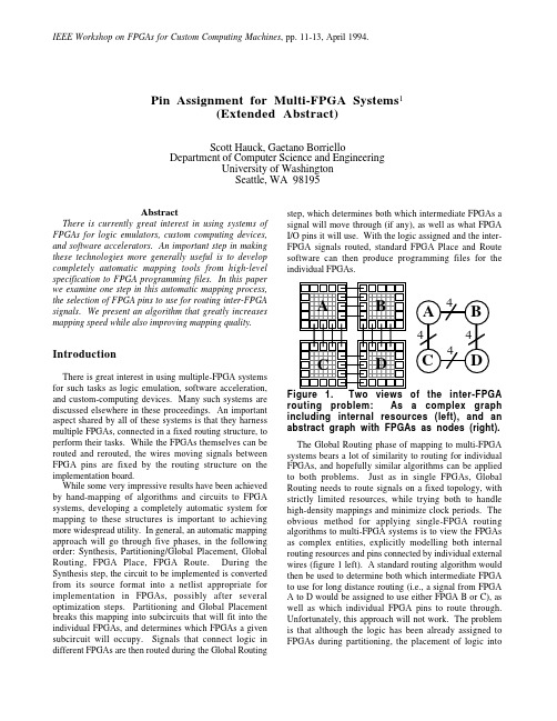
IEEE Workshop on FPGAs for Custom Computing Machines, pp. 11-13, April 1994.Pin Assignment for Multi-FPGA Systems1(Extended Abstract)Scott Hauck, Gaetano BorrielloDepartment of Computer Science and EngineeringUniversity of WashingtonSeattle, WA 98195AbstractThere is currently great interest in using systems of FPGAs for logic emulators, custom computing devices, and software accelerators. An important step in making these technologies more generally useful is to develop completely automatic mapping tools from high-level specification to FPGA programming files. In this paper we examine one step in this automatic mapping process, the selection of FPGA pins to use for routing inter-FPGA signals. We present an algorithm that greatly increases mapping speed while also improving mapping quality. IntroductionThere is great interest in using multiple-FPGA systems for such tasks as logic emulation, software acceleration, and custom-computing devices. Many such systems are discussed elsewhere in these proceedings. An important aspect shared by all of these systems is that they harness multiple FPGAs, connected in a fixed routing structure, to perform their tasks. While the FPGAs themselves can be routed and rerouted, the wires moving signals between FPGA pins are fixed by the routing structure on the implementation board.While some very impressive results have been achieved by hand-mapping of algorithms and circuits to FPGA systems, developing a completely automatic system for mapping to these structures is important to achieving more widespread utility. In general, an automatic mapping approach will go through five phases, in the following order: Synthesis, Partitioning/Global Placement, Global Routing, FPGA Place, FPGA Route. During the Synthesis step, the circuit to be implemented is converted from its source format into a netlist appropriate for implementation in FPGAs, possibly after several optimization steps. Partitioning and Global Placement breaks this mapping into subcircuits that will fit into the individual FPGAs, and determines which FPGAs a given subcircuit will occupy. Signals that connect logic in different FPGAs are then routed during the Global Routing step, which determines both which intermediate FPGAs a signal will move through (if any), as well as what FPGA I/O pins it will use. With the logic assigned and the inter-FPGA signals routed, standard FPGA Place and Route software can then produce programming files for the individual FPGAs.Figure 1. Two views of the inter-FPGA routing problem: As a complex graph including internal resources (left), and an abstract graph with FPGAs as nodes (right).The Global Routing phase of mapping to multi-FPGA systems bears a lot of similarity to routing for individual FPGAs, and hopefully similar algorithms can be applied to both problems. Just as in single FPGAs, Global Routing needs to route signals on a fixed topology, with strictly limited resources, while trying both to handle high-density mappings and minimize clock periods. The obvious method for applying single-FPGA routing algorithms to multi-FPGA systems is to view the FPGAs as complex entities, explicitly modelling both internal routing resources and pins connected by individual external wires (figure 1 left). A standard routing algorithm would then be used to determine both which intermediate FPGA to use for long distance routing (i.e., a signal from FPGA A to D would be assigned to use either FPGA B or C), as well as which individual FPGA pins to route through. Unfortunately, this approach will not work. The problem is that although the logic has been already assigned to FPGAs during partitioning, the placement of logic intoindividual logic blocks will not be done until the next step, FPGA placement. Thus, since there is no specific source or sink for the individual routes, standard routing algorithms cannot be applied.The approach we take here is to abstract entire FPGAs into single nodes in the routing graph, with the arcs between the nodes representing bundles of wires. This solves the unassigned source and sink problem mentioned above, since while the logic hasn’t been placed into individual logic blocks, partitioning has assigned the logic to the FPGAs. It also simplifies the routing problem, since the graph is much simpler, and similar resources are grouped together (i.e. all wires connecting the same FPGAs are grouped together into a single edge in the graph). Unfortunately, the routing algorithm can no longer determine the individual FPGA pins a signal should use, since those details have been abstracted away. It is this problem, the assignment of interchip routing signals to FPGA I/O pins, that the rest of this paper addresses. Pin assignment for multi-FPGA systems One solution to the pin assignment problem is quite simple: ignore it. After Global Routing has routed signals through intermediate FPGAs, those signals are then randomly assigned to individual pins. While this simple approach can quickly generate an assignment, it gives up some optimization opportunities. A poor pin assignment can not only result in greater delay and lower logic density, but can also slow down the place and route software, which must deal with a more complex mapping problem.A second solution is to use a topology that simplifies the problem. Specifically, topologies such as bipartite graphs only connect logic-bearing FPGAs with routing-only FPGAs. In this way, the logic-bearing FPGAs can be placed initially, and it is assumed that the routing-only FPGAs can handle any possible pin assignment. More details on such an approach can be found in [1]. However, it is important to note that these approaches only apply to topologies such as bipartite graphs and partial crossbars, topologies where logic-bearing FPGAs are not directly connected.A third approach is to allow the FPGA placement tool to determine its own assignment. This requires that the placement tool allow the user to restrict the locations where an I/O pin can be assigned (e.g., Xilinx APR and PPR placement and routing tools [4]). With such a system, I/O signals are restricted to only those pin locations that are wired to the proper destinations. Once the placement tool determines the pin assignment for one FPGA, this assignment is propagated to the attached FPGAs. It is important to note that this does limit the number of placement runs that can be performed in parallel. Specifically, since the assignment from one FPGA is propagated to adjacent FPGAs only after that entire FPGA has been placed, no two adjacent FPGAs can be placed simultaneously. Since the placement and routing steps can be the most time-consuming steps in the mapping process, achieving the greatest parallelism in this task can be critical. Also, while the iterative placement approach can optimize locally, creating good results in a single FPGA, it ignores more global optimization opportunities. Finally, there are some topologies for which iterative placement may be unable to determine a correct pin assignment, because the placement of one FPGA may use up resources required in another FPGA. Force-directed pin assignment for multi-FPGA systemsAs we have discussed, pin assignment via sequential placement of individual FPGAs can be slow, cannot optimize globally, and may not work at all for some topologies. What is necessary is a more global approach which optimizes the entire mapping, while avoiding sequentializing the placement step. Intuitively, the best approach to pin assignment would be to simultaneously place all FPGAs, with the individual placement runs communicating with each other to balance the pin assignment demands of each FPGA. In this way a global optimum could be reached, and the mapping of all FPGAs would be completed as quickly as any single placement could be accomplished. Unfortunately, tools to do this do not exist, and the communication necessary to perform this task could become prohibitive. Our approach is similar to simultaneous placement, but we will perform the assignment on a single machine within a single process. Obviously, with the placement of a single FPGA consuming considerable CPU time, complete placement of all FPGAs simultaneously on a single processor is impractical, and thus simplification of the problem will be key to a workable solution.Our approach is to use force-directed placement of the individual FPGAs [3]. In force-directed placement, the signals that connect logic in a mapping are replaced by springs between the signal’s source and each sink, and the placement process consists of seeking a minimum net force placement of the logic. By finding this minimum net force configuration, we expect to minimize wirelength in the resulting mapping. To find this configuration, the software randomly chooses a logic block and moves it to its minimum net force location. This hill-climbing process continues until a local optimum is found, at which point the software accepts the current configuration.Force-directed placement may seem a poor choice for pin assignment, and is generally felt to be inferior tosimulated annealing for FPGA placement. Two reasons for this are the difficulty force-directed placement has with optimizing for goals other than wirelength, and the inaccuracy of the spring approximation to routing costs. However, force-directed placement can handle all of the optimization tasks involved in pin assignment, and the spring metric is the key to efficient handling of multi-FPGA systems.Figure 2. Example of spring simplification rules. Source circuit at top has node U replaced at middle, and any springs created in parallel to others are merged at bottom.As implied earlier, we will not simply place individual FPGAs, but will in fact use force-directed placement simultaneously on all FPGAs in the system. To make this tractable, we can simplify the mapping process. Specifically, since we are only performing pin assignment, we do not care where the individual logic blocks are placed. Thus, we can examine the system of springs built for the circuit mapping, and use the laws of physics to remove nodes corresponding to FPGA logic blocks, leaving only I/O pins. As shown in the example of figure 5, the springs connected between an internal logic node and its neighbors can be replaced with a set of springs connected between the node’s neighbors while maintaining the exact same forces on the other nodes. By repeatedly applying these simplification rules to the logic nodes in the system, we end up with a mapping consisting only of I/O pins, with spring connections that act identically to the complete mapping they replace. In this way, we simplify the problem enough to allow the pin assignment of a large system of FPGAs to be performed efficiently.We have performed comparisons of our force-directed approach with iterative placement approaches, as well as random pin assignments, on several current multi-FPGA systems. The results have shown that the force directed approach is faster than all other alternatives, including random, by up to almost a factor of ten. It also produces higher-quality results than the other approaches, yielding up to an 8.5% decrease in total wirelength in the system. Our algorithm works on arbitrary topologies, including those for which iterative placement approaches generate incorrect results. Complete results, along with a more thorough discussion of this topic, can be found in [2]. References[1] P. K. Chan, M. D. F. Schlag, "Architectural Tradeoffs in Field-Programmable-Device-Based Computing Systems", IEEE Workshop on FPGAs for Custom Computing Machines, pp. 152-161, 1993.[2] S. Hauck, G. Borriello, "Pin Assignment for Multi-FPGA Systems", University of Washington, Dept. of Computer Science & Engineering Technical Report #94-04-01, April 1994.[3] K. Shahookar, P. Mazumder, “VLSI Cell Placement Techniques”, ACM Computing Surveys, Vol. 23, No. 2, pp. 145-220, June 1991.[4] Xilinx Development System Reference Guide and The Programmable Logic Data Book, Xilinx, Inc., San Jose, CA, 1993.1 This paper is an extended abstract of University of Washington, Dept. of Computer Science & Engineering Technical Report #94-04-01, April 1994.。

WRCP

Achieving fast convergence for max-min fair rate allocation in Wireless Sensor NetworksAvinash Sridharan and Bhaskar Krishnamachari{asridhar,bkrishna}@Dept.of Electrical Engineering,University of Southern CaliforniaABSTRACTThe state of the art congestion control algorithms for wire-less sensor networks respond to coarse-grained feedback re-garding available capacity in the network with an additive in-crease multiplicative decrease mechanism to set source rates. Providing precise feedback is challenging in wireless net-works because link capacities vary with trafﬁc on interfering links.We address this challenge by applying a receiver ca-pacity model that associates capacities with nodes instead of links,and use it to develop an iterative algorithm that prov-ably converges to lexicographic max-min fair rate allocation. We use this algorithm as the basis for the design and imple-mentation of theﬁrst explicit and precise distributed rate-based congestion control protocol for wireless sensor net-works—the wireless rate control protocol(WRCP),which can operate in asynchronous networks with dynamic trafﬁc conditions.We show through extensive results from experi-ments that WRCP offers substantial improvements over the state of the art inﬂow completion times as well as in end-to-end packet delays.1.INTRODUCTIONIn event driven sensor networks,one of the primary modes of operations is for nodes to remain dormant for long dura-tions,and becoming active for short durations on sensing an event.In order to reduce the lag between sensing at the edges and detection at the base station,it is imperative to get the sensed data efﬁciently to base station within the uptime of the network.The duration of uptime in these networks has signiﬁcant ramiﬁcations on the network life time.Apart from event driven sensor networks,networks that are con-tinuously monitoring the environment need to employ duty cycling when they require to achieve network life times to the order of years.For such networks,data sensed during the dormant phase is stored on boardﬂash,bulk data trans-fer then takes place during the periodic wake up phase of the network.A characteristic of sensor networks in general, is the low data rates that these networks operate at(∼250 kbps/sec).Due to interference,even in networks that are as small as20nodes,the per node available rate is to the order of2pkts/sec(where the packet size is as small as40 bytes).Given the constrained bandwidth resources available,for these class of sensor networks which need to maintain small uptime,it is imperative to have rate control mecha-nisms for fast and efﬁcient delivery of data.In the absence of rate control mechanisms the networks might experience congestion collapse if nodes are greedily aggressive in try-ing to minimize their up time.The occurrence of congestion collapse in event driven systems in the absence of rate con-trol mechanisms has been highlighted in[19]and[18].Fur-ther,for these class of networks,given the requirement of maintaining short uptime,it is important that rate control al-gorithms are responsive and hence exhibit fast convergence times allowing the sources to send at the achievable rate as fast as possible.In wireless sensor networks the philosophy of performing congestion control has largely been based on a router-centric approach which uses explicit congestion feedback from in-termediate nodes.However,existing schemes still assume a lack of knowledge of achievable network capacity.The key reason has been the difﬁculty in computing capacity given that the bandwidth of each link is affected by interference from other links in its vicinity.The core AIMD mechanism is therefore a component of nearly all distributed conges-tion control protocols proposed for wireless sensor networks (ARC[25],CODA[23],FUSION[12],IFRC[19]).AIMD-based schemes have the advantage that the proto-col is agnostic to the underlying link layer,allowing for mod-ular protocol design.They can also be designed to guaran-tee efﬁcient and fair rate allocation in steady state.However, AIMD mechanisms take a long time to converge and can ex-hibit long queue backlogs as the rates constantly exceed the available capacity(which is required to obtain a signal from the network that it is time to cut back).This is illustrated in Figure1,which presents the performance of IFRC[19], the state of the art for congestion control in wireless sensor networks,in a simple4-node experiment(see Figure6).In this particular example it can be observed that the rate allo-cation takes more than300seconds to converge,and queue sizes routinely reach8-10packets.We therefore believe that a fresh look at the problem of rate control design for sensor networks is required,with emphasis on convergence times and end-to-end packet delays.Our principal contribution in this work is the design of aFigure1:The behavior of allocated rate and queue back logs for IFRC.distributed rate control protocol,that we refer to as the Wire-less Rate Control Protocol(WRCP),which uses an ap-proximation of the available capacity in order to provide ex-plicit and precise feedback to sources.This approximation is obtained by exploiting knowledge of the performance of the underlying CSMA MAC protocol.The key idea in our ap-proach is to associate a constant capacity with nodes instead of links.The gains of this approach in terms of convergence times(few tens of seconds for WRCP as compared to hun-dreds of seconds for IFRC)and smaller queue back logs are highlighted in Figure2.The fast convergence times trans-lates to fastﬂow completion times and the reduced queue size improves end-to-end packet delays.The rest of the paper is organized as follows.First,in section2,we present a useful notion of capacity in a wire-less sensor network operating a CSMA protocol,which is referred to as receiver capacity.This determines the con-straints that deﬁne an achievable rate region forﬂows in a collection tree.In Section3we describe a idealized syn-chronous algorithm,which acts as the motivation for the WRCP protocol,and which provably converges to a lexico-graphic max-min fair rate allocation under this receiver ca-pacity ing the intuition presented by the idealized algorithm(section3)we design the Wireless Rate Control Protocol,presented in Section4,which handles real-world concerns of asynchrony,trafﬁc-dynamics and stochastic in the underlying network,link and physical layers.We then describe the software architecture of WRCP(in Section5), which is designed to be integrated easily with the TinyOS2.x collection tree architecture for wireless sensor networks.We undertake an experimental evaluation of WRCP on Tmote Sky devices using the IEEE802.15.4-compliant CC2420ra-dios.We give details of our experimental methodology in Section6.We then compare our protocol extensively over both static and dynamic-trafﬁc scenarios with IFRC,the state of the art distributed rate control protocol for wireless sensor networks,over a20-node experimental testbed(Section7). The results show substantial improvements inﬂowcomple-Figure2:The behavior of allocated rate,queue back logs for WRCP.tion times and end-to-end packet delays.We place our con-tributions in light of prior work in Section8,and present concluding comments on future work in Section9.2.RECEIVER CAPACITYThe primary requirement for designing an explicit and precise rate control algorithm is a usable notion of achiev-able capacity.In traditional wired networks,the notion of capacity is associated with a link existing between any two nodes.Allﬂows traversing the link are assumed to linearly share the constant capacity of the link.In wireless networks the capacity of a link is not constant,but rather affected by activity on interfering links in its vicinity.We therefore need to redeﬁne the notion of capacity.Each node can be perceived as having a receiver domain consisting of all transmitting nodes within range,including itself.The crux of our approach is to associate the concept of capacity with nodes instead of links,we refer to this as receiver capacity.This capacity is to be shared linearly by allﬂows traversing the corresponding receiver’s domain.Al-though in general the region of achievable rates in a given re-ceiver domain is not linear,we approximate it with a linear rate region by making the receiver capacity a constant that depends only upon on the number of neighboring nodes(not their rates).Although we believe on intuitive grounds that this is a good approximation for wireless sensor networks due to the small packet sizes(≈40bytes)that are prevalent in such networks,we do not prove here rigorously how good this approximation is.We rely on the empirical results pre-sented in our evaluation of WRCP which is designed based on this approximation,to show that it is extremely useful in practice.Most sensor networks today use a randomized CSMA MAC as the de facto data link layer.In order to associate a value to the receiver capacity,we equate the capacity of a receiver with the saturation throughput of the CSMA MAC.The sat-uration throughput[5]of a CSMA MAC is deﬁned as the throughput observed by the receiver when all senders are10 20 30 40 50 60 70 80 90 100 110 120 130 140 150 160 170 180 190 200 1 2 3 4 5 6 7 8 9 10 11 12 13 14 15 16 17 18 19 20 21 22 23 24 25S a t u r a t i o n T h r o u g h p u t (P k t s /s e c )Number of SendersFigure 3:Saturation throughput for multi-ple senders for the CC2420CSMA MAC on TinyOS-2.0.2.2backlogged and are within each others interference range.While this does not cover all possible sender-conﬁgurations possible in a receiver domain,our experience with WRCP shows that although this estimate is potentially conservative,it leads to equal or better performance in terms of achievable goodput compared to the state of the art.Our implementation is performed on the Tmote sky mote [1],which use the CC2420radios,running TinyOS-2.0.2.2.Fig-ure 3presents the empirically measured saturation through-put for this platform as the number of senders in-range is varied.This graph allows us to associate a value with the receiver capacity for each node in a WSN collection ing the notion of receiver capacity,we can determine constraints on rate allocation to ﬂows in a WSN collection tree.Let N i be the set of all neighbors of i (consisting of i itself,all its immediate children,and all other nodes in its interference-range);C i the set denoting the subtree rooted at i (including itself);r i the rate at which data generated at source node i is being transmitted;and B i the value of node i ’s receiver capacity.The receiver capacity constraint at a node i is then given as follows:j ∈N ik ∈C jr k ≤B i (1)We explain this with an example.Figure 4shows an 8node topology.The solid lines indicate a parent-child rela-tionship in the tree.The dashed lines are interference links.Rates indicated on interference links 1quantify the amount of interference generated by a neighboring node when it is transmitting data to its parent.Thus,when node 2sends its data to node 1at some rate,node 2not only consumes the corresponding amount of capacity at node 1but also at node 3;the rate label on interference link 2→3is the same as that on link 2→1.Based on our model,the constraint on the rates at node 3would be as follows:r tot 2+r tot 3+r 6≤B 3(2)where B 3is the receiver capacity of node 3and r 6is theDefinition 2.Max-Min Fair Rate Vector We say a feasible rate vector is max-min fair,if for each i,r i cannot be increased while maintaining feasibility without decreasing r j for some source j for which r j≤r i Intuitively,a max-min fair rate allocation ensures that the most-starved node gets as much rate as possible;conditioned on this,it then ensures that the second most-starved node gets as much rate as possible;and so on.Weﬁrst present an illustrative example to show how this objective can be achieved in the toy8node topology of Figure4.We then present a general iterative distributed algorithm and prove that it will ensure that source rates converge to a rate alloca-tion that is max-min fair for a WSN collection tree under the receiver capacity model.3.1An Illustrative ExampleTo determine the max-min fair rate allocation for the topol-ogy of Figure4,weﬁrst need to calculate the perﬂow avail-able capacity at each node.For this calculation we divide the receiver capacity at each node by the total number ofﬂows incident and exiting the node.For example there are4ﬂows incident on node2(2from4and5,and2from node3),and 3ﬂows exiting node2(2from its children and1of its own), giving a totalﬂow count at node2of7.Thus,the perﬂow available capacity for node2is B26,for node7it would be B74,B53and B87≥B37since the sum would add up toB2and allﬂows at node2would get an equal share.In the given topology this would apply toﬂows from nodes2,3, 4,5and6.Flows from nodes7and8do not consume node 2’s bandwidth and hence their rates should be constrained bynode7(assuming B73),resulting inﬂows from7and8being allocated a max-min rate of B7Pj∈N iF j2.γmini(n+1)=minj∈Sγj(n+1)3.γpathi(n+1)=minj∈A iγj(n+1)4.ifγpathi(n+1)>05.then r i(n+1)=r i(n)+γmini(n+1)•F i is the the total number ofﬂows forwarded by nodei,whoseγpath>0.F i counts only thoseﬂows whodo not have a single node in their path whose capacityhas been exhausted.•S is the set of all nodes i whoseγi>0.Theorem 1.Algorithm MMF-RC converges in aﬁ-nite number of steps.Proof.At every time step n,in step2of MMF-RC a node i is picked whoseγi(n)>0and is the minimum amongst the set S.In step3every source k calculates itsγpathk(n),which corresponds to the minimum of the avail-able perﬂow capacity amongst all nodes in the set A k,whosebandwidth source k consumes.Every source k whoseγpathk> 0increments its allocated rate r k(n)byγi(n).Thus,at time step n since allﬂows in the set F i have increased their rates byγi(n)>0,at time step n+1,γi(n+1)=0.Thus, at time step n+1all sources k which have i∈A k willhaveγpathk=0and hence will not increase their rate after time step n+1.Since i was any arbitrary node and n was any arbitrary time step,for n>0at every n+1time stepthere will be at least1source k,whoseγpathk(n+1)=0. Since the total number of sources in the system areﬁnite, in aﬁnite number of steps N′>N,where N is the total number of source’s in the system,all sources i in the systemwill haveγpathi(N′)=0and hence MMF-RC will have converged.Definition 3.We say a node i is a bottleneck node with respect to a source j whoseﬂow consumes band-width at i if its receiver capacity is completely consumed and r j≥r k for all sources k whoseﬂow consumes band-width at i.Lemma 1.A feasible rate vector is max-min fair if and only if in the rate vector every source has a bottle-neck node.We omit a proof of this lemma due to space limitations, but note that it can be proved by a fairly straightforward modiﬁcation of the similar proposition in Section6.5.2of [4]which applies to max-min fair rate allocation in wired networks.The key differences are in substituting bottleneck nodes instead of bottleneck links,and the set A i of all nodes whose bandwidth is consumed by aﬂow instead of the set of links on the path.Theorem 2.The rate vector that Algorithm MMF-RC converges to is max-min fair.Proof.From lemma1,it sufﬁces to show that each node has a bottleneck node when??converges.In theorem1it was shown that at every step n>0,there will be at least one source k whoseγpathk(n)=0,such thatγpath k (n−1)>0.Also,the node k would have increasedits allocated rate by someγmin(n−1)at time step n−1sinceγpathk (n−1)>0.We claim that the node i,whoseγi(n−1)=γmin(n−1),will be the bottleneck node for node k,since at time step nγi(n)=0and till time step n all ﬂows j who were consuming capacity at node i,and whoseγpath j (n−1)>0were experiencing equal increments.Thus,there can be noﬂow j,for whom i∈A j such that r j(N′)> r k(N′)for N′>n.Hence our claim that i is the bottleneck node of k is justiﬁed.Further,since for some N′′>N,where N is the totalnumber of sources,for all sources j,γpathj (N′′)=0,atN′′all sources j will have a bottleneck node.Thus,from lemma1,for some N′′>N MMF-RC converges to the max-min fair rate vector.4.THE WIRELESS RATE CONTROL PRO-TOCOLIn Section3,we presented the MMF-RC algorithm and showed that it achieves max-min fairness over a collection tree.However that algorithm operates in an idealized setting;it assumes synchronous execution,rapid global coordina-tion,constant-bit-rate staticﬂows from backlogged sources, and lossless links.A real world sensor network on the other hand would have asynchronous communication,stochastic introduced due to randomized CSMA MAC,lossy links and dynamicﬂows which might result from the on-demand na-ture of the sensing application.To implement the algorithmin a practical setting,we need to relax these assumptions.To this end we have designed the Wireless Rate Control Protocol(WRCP)which incorporates a number of mech-anisms to handle these real-world concerns.A single time step execution of the protocol is presented in the form of the WRCP algorithmSome additional notation used in the description of the WRCP algorithm is as follows;P i is the parent of node i;r i is the maximum allocated rate at whichﬂows consuming ca-pacity at node i can operate;r tot i is total transmission rateof node i,it is essential to note that for a source its de-mand might be less then its allocated rate,which implies that r tot i≤ j∈C i,∀j r i.Algorithm WRCP1.Calculate Per Flow Available Capacity:2.γi((n+1)T)=B i(nT)−Pj∈N i(nT)r totj(nT)Pj∈N i(nT)F j(nT)7.RateT hresh=0.1×MaxRate8.if r i(nT)>r Pi(nT)9.then r i(nT)=r Pi(nT)10.if r i(nT)≤MaxRate11.then ifγmini((n+1)T)<−RateT hresh12.orγmini((n+1)T)>013.thenα=αdef ault14.elseα=015.if r i(nT)>MaxRate16.then ifγmini((n+1)T)<017.thenα=0.518.else ifγmini((n+1)T)>RateT hresh19.thenα=αdef ault20.elseα=021.r i((n+1)T)=r i(nT)+α×γmini((n+1)T)22.Broadcast to j∈N i:23.γi((n+1)T),γmini((n+1)T),r i((n+1)T)WRCP retains the essential elements of the MMF-RC algorithm(steps2,4,21)and builds on it.Wedescribe the essential components of this protocol be-low.4.1Local TimersWRCP relies on a T second timer to present nodeswith an interval to calculate their rate updates.Intu-itively T should be large enough for a node to be ablegather information from all nodes in the set A i in orderto perform accurate rate updates.Thus,T should beatleast as large as the delay in sending information fromthe sink to the leaf at the largest depth.4.2Estimating Receiver CapacityAs mentioned earlier,we approximate the receivercapacity by the saturation throughput,which is a func-tion of the number of senders in the receiver’s range.The saturation throughput function is pre-calculatedand stored as a lookup table.Figure3shows that thereceiver capacity will almost remain a constant as longas the number of senders is greater than4.4.3Estimating Active Flow CountsIn a dynamic environment,the number of active neigh-bors and the number of activeﬂows in a given neighbor-hood is going to change.To handle the ephemeralﬂowcount,an activeﬂow state tag is associated with eachneighbor entry and aging this entry in the absence ofpackets from the neighbor helps give a correct estimateof activeﬂows in the network.The number ofﬂows in aneighborhood determine the perﬂow available capacityat a receiver.A conservativeﬂow count will calculateﬂows from all the senders that a node has heard fromwithout regard for their link quality.The active neigh-bor andﬂow count is estimated by looking up both thetotal number of active neighbors,and the active sourcesthat each neighbor is forwarding.However,recent em-pirical results have shown that capture eﬀects are quitedominant in these networks[21].These results suggest that nodes with stronger links will cause more inter-ference(or consume more capacity)than nodes with weaker links.We therefore take an optimistic approach and weigh the number ofﬂows from a sender j to a re-ceiver i by its link quality p ij∈[0,1].Our experimental results(section7)show that this gives us a much better estimate of the achievable max-min rate than adoptinga conservative approach.4.4Estimating Transmission RatesDue to the stochastic introduced by random access CSMA schemes which are common in sensor networks, as well as stochastic that might be introduced due to non CBR traﬃc,instantaneous estimates of transmis-sion rates would be erroneous.Hence we maintain an exponential weighted moving average of transmission rates instead of instantaneous estimates as follows:P kts T ransmitted r tot i((n+1)T)=(1−β)r tot i(nT)+βFigure5:Software Architecture for WRCP guarantee the stability and performance of WRCP as well.Since the primary objective of this work is to show that explicit capacity rate control algorithms can be de-signed for sensor networks using a simple model such as the receiver capacity model,we perceive the complete evaluation of parameter selection process for WRCP tobe out of the scope of the current work and target it as part of our future work.For empirical evaluation,we have set the parameters for WRCP intuitively.SinceT needs to cater to the largest delay in the maximum size network that WRCP is going to be operational in, we set it to1000ms(the largest network we have con-sidered is a20node network with4hops).To ensure stabilityαneeds to be set to a small value and the moving average needs to be conservative.Thus,for our evaluation we setα=0.1andβ=0.8.5.SOFTWARE ARCHITECTURE FOR WRCPIN TINYOS-2.XFigure5shows the software architecture of WRCP implementation in TinyOS-2.0.2.2.TinyOS2.0.2.2,al-ready provides a framework for building collection treesin the form of the collection tree protocol(CTP)(TEP 123[2]).Since WRCP aims to achieve lexicographic max-min fairness among sources over a collection tree, we have integrated WRCP with the collection tree pro-tocol.The only modiﬁcation required to the existing MAC (the CC2420CSMA MAC)was the addition ofﬁeldsto the header to support rate control information and provide acknowledgements to broadcast packets using the software acknowledgement feature of TinyOS2.0.2.2 (TEP126[3]).We also modiﬁed the routing engine in CTP to store additional per-neighbor information re-quired by WRCP(current transmission rate,per-ﬂow available capacity,current allocated per-ﬂow rate,ac-tiveﬂow state,number of descendants).We also had to make a major modiﬁcation to the forwarding engine of CTP,since the default forwardingFigure6:A4-node fully connected linear topol-ogy.engine of the collection tree protocol does not imple-ment a FIFO queue.It implements a form of priority queuing which restricts the number of packets originat-ing from an application in the node itself to one,giving higher priority toﬂows from its descendants.Since,our algorithm explicitly assumes that the forwarding engine treats allﬂows equally,we needed to implement a vari-ant of the forwarding engine that implements a FIFO queue.In our software architecture,the core functionalityof WRCP is implemented in the Rate Controller.The Rate Controller performs the per-ﬂow rate calculations, and sets the token generation rate on the leaky bucket[4]. The Flow Controller then uses tokens from the leaky bucket to admit packets into the system.6.EXPERIMENTAL METHODOLOGY6.1Basic Experimental SetupOur implementation is performed on the Tmote sky motes,which have CC2420radios,running TinyOS-2.0.2.2.The experiments are conducted over a small stand alone4-node topology(Figure6)and a larger20-node topology(Figure7)on the USC TutorNet testbed[15]. The smaller topology highlights the behavior of WRCP when a small number ofﬂows exist,pertaining to a scenario when the perﬂow available capacity is high. The larger topology is representative of a network witha large number ofﬂows,pertaining to a scenario witha small available perﬂow capacity.Experiments were conducted over a period of few months to ascertain any change in the performance of the protocols due to link quality variations in the topologies.It was observed that the link quality variations for the topologies over this large time frame were negligible,lending validity to the results.The state of the art for distributed rate control in wireless sensor networks is the Interference Aware Rate Control Protocol(IFRC)[19].We therefore use IFRCas the benchmark for evaluating the performance of WRCP.IFRC is an AIMD scheme and hence a com-parison of WRCP and IFRC will clearly highlight the advantages of designing a rate control protocol in a sensor network setting in terms of allocated rates,Figure7:A20node topology. convergence times,ﬂow completion times and end-to-end delays.To have an unbiased comparison between IFRC and WRCP,we ported IFRC from its TinyOS-1.x2implementation to TinyOS-2.x using the same software architecture used for WRCP(ﬁgure5). Similar to WRCP,IFRC was implemented as the rate controller block in the given software architecture.Due to space constraints we omit the description of IFRC and refer the reader to[19]for protocol speciﬁc details. For comparative evaluation between IFRC and WRCP we consider3scenarios,a static scenario and two dy-namic scenarios.The static scenario pertains to the case whenﬂows are active for the complete duration of the experiment.The two dynamic scenarios highlight the protocol behavior whenﬂow joins andﬂow departures are taking place during the operation of the network. We believe these three cases test the correctness of the protocols(in terms of achieving max-min fair rates)and capture a broad class ofﬂow dynamics that might exist in real sensor networks.7.BENCHMARKING RESULTSFor all experimental results presented in this section, the size of the payload was10bytes.WRCP adds16 bytes,where as IFRC adds26bytes of overhead to each packet.Since both protocols exchange control informa-tion over the data path using a promiscuous mode of operation,WRCP exhibits better overhead eﬃciency. For the purposes of comparison we have set the IFRC parameters r init=0.1pkts/sec,φ=0.0125,ǫ=0.02. The upper queue threshold was set to8packets.These parameters were calculated as per the analysis presented in[19]for a20node topology,since this is the maximum size network we are dealing with in our experiments. For WRCP we setα=0.1,as per the arguments pre-sented in section4.6,and T was set to1000ms to cater2 4 6 8 10 12 14 16 18 20 22 24 26 28 30 0 200 400 600 800 1000 1200 1400A l l o c a t e d R a t e (P k t s /s e c )Time (secs)Src 2 Allocated Src 3 Allocated Src 4 Allocated(a)IFRC rate alloca-tion. 02 4 6 8 10 12 14 16 18 20 22 24 26 28 30 0100200300400500600700800900100011001200130014001500A l l o c a t e d R a t e (P k t s /s e c )Time (secs)Src 2 Allocated Src 3 Allocated Src 4 Allocated(b)WRCP rate alloca-tion. 05000 10000 15000 20000 2500030000 01002003004005006007008009001000110012001301400N u m b e r o f P a c k e t s R e c i e v e d a t B STime (secs)WRCP Src 4 Flow Completion IFRC Src 2 Flow Completion(c)WRCP and IFRC ﬂow completion times.Node ID(d)WRCP and IFRC goodput.(e)WRCP and IFRC end-to-end packet delayFigure 8:The convergence time of the allocated rate,ﬂow completion time,goodput and end-to-end packet delay for WRCP and IFRC on the 4-node fully connected topology,in a static scenario.2 4 6 8 10 030060090012001500A l l o c a t e d R a t e (P k t s /s e c )Time (secs)Src 2 Allocated (One hop)Src 18 Allocated (Two hops)Src 19 Allocated (Three hop)Src 20 Allocated (Four hops)(a)IFRC rate alloca-tion. 02 4 6 8 10 030060090012001500A l l o c a t e d R a t e (P k t s /s e c )Time (secs)Src 2 Allocated (One Hop)Src 18 Allocated (Two Hops)Src 19 Allocated (Three Hops)Src 20 Allocated (Four Hops)(b)WRCP rate alloca-tion. 01000 2000 3000 4000 5000 6000 0100200300400500600700800900100011001200130014001500N u m b e r o f P a c k e t s R e c i e v e d a t B STime (secs)WRCP Src 2 Packet Completion IFRC Src 2 Packet Completion WRCP Src 17 Packet Completion IFRC Src 17 Packet Completion(c)Flow completion times.A v e r a g e R a t e (P k t s /s e c )Node ID(d)Goodput.A v e r a g e D e l a y (m s )Node ID(e)End-to-End packetdelays.Figure 9:The convergence time of the allocated rate,ﬂow completion time,goodput and average delay for WRCP and IFRC on the 20-node topology when all ﬂows start simultaneously (static scenario).and ??.The ﬂow dynamics for this experiment are as follows:•Flows from sources 2,3,8and 12(ﬁrst hop sources)start at the beginning of the experiment and re-main active for the complete duration of the ex-periment.•Flows from sources 5,6,9,11,14,15,18,4,10(second hop sources)become active after the ﬁrst 1000seconds.•Flows from sources 7,13,16and 19(third hop sources)become active after the ﬁrst 2000seconds.•Flows from sources 17and 20(fourth hop sources)become active after the ﬁrst 3000seconds.In this experiment all nodes keep their rate controllers on from the start of the experiments.For IFRC,the advantage of the rate controllers always being on,irre-spective of whether a node is sending out a ﬂow or not,is that rates are pre-computed,and hence,when a ﬂow joins the network it starts a much higher rate exceeding network capacity and forcing sources to perform multi-plicative decrease (since the rates computed before the ﬂow joined the network was for a smaller number of ﬂows).This leads to faster convergence times in terms of the allocated rate.However,it leads to a patho-logical case which can be seen in Figure 10(a)at 3000Node IDFigure 11:Goodput (Case 1).seconds.If the congestion is large,due to multiple ﬂow joins,and the multiplicative decrease of IFRC is not ag-gressive enough,it might lead to the multiplicative de-crease setting the threshold value([19])quite low.Since the rate controllers have always been on,all nodes in the network are in the additive increase phase.In this phase,since the rate of increase is solely dependent on the threshold value value,the slope of the increments is severely aﬀected by the excessive congestion experi-enced by sources.For WRCP,the above scenario does not present a problem since the number of ﬂows are actively com-puted and even though ﬂows start at a higher rate the decrements are aggressive and accurate,since the。

抽象词

Exmaple:…be a descryiptive distinction rather than an empirical observation and consequently lacks explanatory value.
这句话所用的单词大家都认识，可是为什么不易读懂呢？就在于构成这句话的单词全是一些这样的抽象词，下面列了一些抽象词，大家看一看，有没有大家不认识的？
问题我们已经找出来了，该如何云解决呢？
阅读抽象词训练法
第一步、在阅读完每一篇GRE或GMAT文章之后，按照上面所说的三个标准找出这些抽象词来。
第二步、把这些单词记在小本上或存在电脑里，也可以补充到本书所列的三百多个抽象词中；读文章或背单词感到疲劳了，就可以拿来翻一翻，想一想。
注意这里所说的想的方法。比如在刚才作为例子所举出的抽象词中的appraise，大家应该都知道其中文释义叫做评估，可是如果你只知道在现场的阅读中把翻译成中文的评估，再云想评估的意思是什么，这种速度是无法满足GRE或GMAT考试对阅读的要求的。那么什么叫appraise呢？比如说这瓶矿泉水，我们对其评估的过程是这样的：先把它拿出来观察，找出其性质特点与同类(或一个标准)作比较，根据优缺点对共价值做出估测，然后再找到它在当前市场情况下的合理价位，这么一个完整的过程才叫做appraise，如果我们到考场上去把appraise翻译成评估，再云想这个过程，纯属浪费时间；最快的方法，就是一看到appraise这个单词，你就下意识地直觉性地反映出这样一个过程来。
GRE和GMAT文章的特殊性就在于涉及的因素之多，是其他任何部分都无法与之相比的，因此才在两种考试中都成为最难的一个部分。如果说文章是高楼大厦，段落就是房间，句子就是一面面的墙，单词就是一块块的砖。以上几个环节中的任何一个环节出了问题，都会影响我们对整篇文章的理解。为了解决上述问题，本书着重研究了如何克服GRE或GMAT难句的问题，这里来谈一谈单词的问题。

Scenario reduction in stochastic programming_ an approach using probability

1. Introduction Various important real-life decision problems can be formulated as convex stochastic programs which can be mostly written in the form min EP f (ω, x) =
An approach using probability metrics
Received: July 2000 / Accepted: May 2002 Published online: February 14, 2003 – c Springer-Verlag 2003 Abstract. Given a convex stochastic programming problem with a discrete initial probability distribution, the problem of optimal scenario reduction is stated as follows: Determine a scenario subset of prescribed cardinality and a probability measure based on this set that is the closest to the initial distribution in terms of a natural (or canonical) probability metric. Arguments from stability analysis indicate that Fortet-Mourier type probability metrics may serve as such canonical metrics. Efﬁcient algorithms are developed that determine optimal reduceal experience is reported for reductions of electrical load scenario trees for power management under uncertainty. For instance, it turns out that after 50% reduction of the scenario tree the optimal reduced tree still has about 90% relative accuracy. Key words. stochastic programming – quantitative stability – Fortet-Mourier metrics – scenario reduction – transportation problem – electrical load scenario tree

DISORT

***********************************************************************Documentation File for 'DISORT', A Discrete Ordinates RadiativeTransfer Fortran-90 Program for a Multi-Layered Plane-Parallel Medium (VERSION 1.3)***********************************************************************NOTE: If you have not received DISORT directly from its main anonymous ftp siteftp:///pub/wiscombe/Multiple_Scatt/you should check there for the latest version, and any updates.FORTRAN-90: This is the first version of DISORT requiring a Fortran-90 compiler. So far, the only Fortran-90 actually used is in RDI1MACH.f, since these routines in their f77 form were by far the most unpopular among DISORT users; their f90 implementation, by contrast, is clean andsimple. The rest of DISORT will gradually migrate to Fortran-90, for reasons given in RDI1MACH.readme and in the DISORT Report, Appendix B.Note that any f77 code can be compiled by an f90 compiler, as long as the filename has a .f extension indicating fixed source form.Those without access to an f90 compiler can either(a) use version 1.2; or(b) use this version but substitute R1MACH.f and D1MACH.f from version1.2.Send us e-mail if you find that, after a reasonable effort, you cannot gain access to an f90 compiler; this will help us understand the extent to which f90 compilers are available (or not) among our user base.----------------------------------------------------------------------CODE HISTORY:version 1.0, 1988 (Fall): built upon code foundation developed by Si-cheeTsay in his thesis under Knut Stamnes, largely during an intensefour-weekvisit by Wiscombe to the University of Alaska, Fairbanks;version 1.1 1993 (Jan): small bug fixes since 1988, mostly in ASYMTX and IBCND=1 special case; NCUT option no longer applied if thermal emission present; zero optical depth layers handled better; other mostly cosmetic changes (printing formats, etc.)version 1.2, 1997 (Feb): put under RCS control; many small cosmetic changes; ALBTRN and SOLVE1 reorganized; fewer significant digits printed in test problems, in order to reduce trivial differenceswhen comparing two outputs; in test problems, SIGNIFICANTLY NON-UNIT RATIOS only counted when flux or intensity above noise level;SQT calculation moved up to DISORT;version 1.3, 2000 (Mar): LAPACK used instead of LINPACK to do linear algebra (but not for eigenvalue problem yet); first Fortran-90 version; R1MACH, D1MACH use Fortran-90 intrinsic functions;(Many thanks to Robert Pincus for the conversion to LAPACK)NOTE: Even though there have been many small changes to DISORT,there have been no significant bug reports for many years. Thebugs found have tended to be obscure and unlikely to affect the vast majority of users in any significant way.-------------------------------------------------------------------This program package consists of the following files (in addition to the file you are reading, DISORT.doc):DISORT.fThe user entry point (subroutine DISORT), and most of the routines it calls. All routines are in single precision except for theeigenvalue routine ASYMTX and the quadrature-angles routine QGAUSN.DISORTsp.fLike DISORT.f, but EVERYTHING is in single precision. Singleprecision may be adequate for many applications, but this variantis also necessary if you want to use the auto-doubling option now available on many compilers (if you auto-double, however, you needtochange all instances of 'R1MACH' to 'D1MACH'). This is also the version to use on Cray and other high-accuracy machines.DISOTEST.fA program for checking DISORT on a comprehensive set of test problems. Be sure to run this before using DISORT.DISOTEST.docDocumentation for DISOTEST.fDISOTEST.outOutput from running DISOTEST.f in normal mixed single-double precisionon an IEEE-arithmetic Unix workstation. Filename may have aversion number included.RDI1MACH.fFortran-90 Routines for returning machine constants, from netlib authorEric Grosse; also see file RDI1MACH.readme.DISORTlapack.fRoutines used by DISORT from the linear-equation-solving public-domainpackage LAPACK. Included only to make DISORT self-contained. The user is encouraged to employ the local compiled LAPACK library (if one exists)rather than this file, because it will be optimized for the local environment. More information about LAPACK is given in the fileLapackBlas.readme.DISORTblas.fRoutines used by DISORT from the Basic Linear Algebra Subroutinespublic-domain package BLAS-1,2,3. Included only to make DISORTself-contained. The user is encouraged to employ the local BLAS library (if one exists) rather than this file, because it will beoptimized for the local environment. Even if there is not a locallyoptimized LAPACK, there may well be a locally optimized BLAS. More information about BLAS is given in the file LapackBlas.readme.ErrPack.fError-handling routines. Standard across almost all programs on the wiscombe anonymous ftp site.rundis1.3Example C-shell script to run DISORT. Shows how to put the various pieces together, and how to handle single, double, and mixed single- double precision runs in an automated way.---------------------------------------------------------------------All the DISORT code has passed tests by 'flint', 'ftnchek', and'nag_pfort' -- tools that test the semantics of Fortran programs at ahigher level than compilers do. These tools were helpful in exposing subtle bugs in DISORT in the early days, and remain useful for ensuring that new bugs are not introduced. 'ftnchek' is free and available from ; the others are commercial products (see the FortranMarket, /) but well worth the investment.Remarks on Computer Precision-----------------------------DISORT has certain intrinsic limitations because of computer precision. These limitations are related to ordinary computer "roundoff error" and have nothing to do with user-controllable (through the number of streams NSTR) "truncation error". DISORTis free of the *catastropic* growth of roundoff error thatplagued pre-1980 discrete ordinate programs, but certain partsof the calculation (the eigenvalue/vector and Gauss quadraturerule computations, and to a much lesser extent the linearequation solving computations) are just inherently more sensitiveto roundoff than the rest of DISORT, because they involve so many arithmetic operations.The reason DISORT.f does the eigenvalue/vector and Gauss quadrature rule computations in double precision is that DISORTwas originally developed on 32-bit-single-precision computers (VAXen and IBMs) which were too inaccurate for those computations. Running DISORT.f on a typical 32-bit-single-precision computer usually gives results precise to at least 2-3 significant digits, although for certain special situations the precision can fall to one significant digit. Results can even have NO significant digits when they fall below about 10**(-8) times the driving radiation, as one can see in the fluxes in some of the test problems.IEEE Underflow: On some Unix workstations (notably an HP9000), turning on certain compiler options can also cause IEEE underflowsto trigger an error condition and abort the test run. On theHP9000, this option was +T, which ostensibly produces a tracebackbut as a side effect bombs the run. DISORT will never pass underflow tests because it has potential underflows all over the place, esp.in the computations of exponentials.Memory Usage------------DISORT defines a considerable number of local arrays, whose default sizes are rather large to accommodate the test problems. The sizeof these arrays can be reduced by the user simply by altering the PARAMETER statements (for MX...) just following the internalvariable documentation in subroutine DISORT. This can give adramatic reduction in memory usage for typical applications.Elimination of this annoyance through use of dynamically dimensioned arrays is one of the first goals of the f90 conversion of DISORT.---------------------------------------------------------------------AUTHORS :Knut Stamnes and Collaborators (kstamnes@)Stevens Institute of TechnologyHoboken, New JerseySi-Chee Tsay (Tsay@)NASA Goddard Space Flight CenterCode 913Greenbelt, MD 20771Warren Wiscombe (Warren.Wiscombe@)NASA Goddard Space Flight CenterCode 913Greenbelt, MD 20771Stuart Freidenreich (vr@)NOAA Geophysical Fluid Dynamics LaboratoryPrinceton, NJ 08540Istvan Laszlo (laszlo@)University of MarylandDept. of MeterologyCollege Park, MD 20742Robert Pincus (Robert.Pincus@)Ran SongNASA Goddard Space Flight CenterCode 913Greenbelt, MD 20771Collaborators: cf. REFERENCES---------------------------------------------------------------------REFERENCES (cited in the programs using the acronyms shown) :DGIS: Devaux, C., Grandjean, P., Ishiguro, Y. and C.E. Siewert,1979: On Multi-Region Problems in Radiative Transfer, Astrophys. Space Sci. 62, 225-233GS: Garcia, R.D.M. and C.E. Siewert, 1985: BenchmarkResults in Radiative Transfer, Transport Theoryand Statistical Physics 14, 437-483L: Lenoble, J., ed., 1985: Radiative Transfer in Absorbingand Scattering Atmospheres: Standard ComputationalProcedures, Deepak Publishing, Hampton, VirginiaNT: Nakajima, T. and M. Tanaka, 1988: Algorithms for Radiative Intensity Calculations in Moderately Thick Atmospheres Using a Truncation Approximation, J.Q.S.R.T. 40, 51-69OS: Ozisik, M. and S. Shouman, 1980: Source FunctionExpansion Method for Radiative Transfer in a Two-Layer Slab, J.Q.S.R.T. 24, 441-449SS: Stamnes, K. and R. Swanson, 1981: A New Look atthe Discrete Ordinate Method for Radiative TransferCalculations in Anisotropically ScatteringAtmospheres, J. Atmos. Sci. 38, 387-399SD: Stamnes, K. and H. Dale, 1981: A New Look at theDiscrete Ordinate Method for Radiative TransferCalculations in Anisotropically ScatteringAtmospheres. II: Intensity Computations,J. Atmos. Sci. 38, 2696-2706S1: Stamnes, K., 1982: On the Computation of AngularDistributions of Radiation in PlanetaryAtmospheres, J.Q.S.R.T. 28, 47-51S2: Stamnes, K., 1982: Reflection and Transmission bya Vertically Inhomogeneous Planetary Atmosphere,Planet. Space Sci. 30, 727-732SC: Stamnes, K. and P. Conklin, 1984: A New Multi-LayerDiscrete Ordinate Approach to Radiative Transferin Vertically Inhomogeneous Atmospheres,J.Q.S.R.T. 31, 273-282SW: Sweigart, A., 1970: Radiative Transfer in AtmospheresScattering According to the Rayleigh Phase Functionwith Absorption, The Astrophysical JournalSupplement Series 22, 1-80STWJ: Stamnes, K., S.-C. Tsay, W. Wiscombe and K. Jayaweera, 1988: A Numerically Stable Algorithm forDiscrete-Ordinate-Method Radiative Transfer inMultiple Scattering and Emitting Layered Media,Appl. Opt. 27, 2502-2509.STWL: Stamnes, K., S.C. Tsay, W. Wiscombe and I. Laszlo:A General-Purpose Numerically Stable ComputerCode for Discrete-Ordinate-Method RadiativeTransfer in Scattering and Emitting Layered Media,to appear as NASA report (1995)VH1,VH2: Van de Hulst, H.C., 1980: Multiple Light Scattering,Tables, Formulas and Applications, Volumes 1 and 2, Academic Press, New York.W: Wiscombe, W., 1977: The Delta-M Method: Rapid YetAccurate Radiative Flux Calculations, J. Atmos. Sci. 34, 1408-1422----------------------------------------------------------------------PREFACEDISORT was designed to be the most general and versatileplane-parallel radiative transfer program available, applicableto problems from the ultraviolet to the radar regions of the electromagnetic spectrum. As such, it has a rather large listof input variables. This list is more easily comprehended if several simple facts are borne in mind :* there is one vertical coordinate, measured in optical depthunits, and two angular coordinates, one polar and one azimuthal;* the layers and polar angles necessary for computationalpurposes are *entirely decoupled* from the levelsand polar angles at which the user desires results.The computational layering is usually constrained by the problem, in the sense that each computational layer must be reasonably homogeneous and not have a temperature variation of more thanabout 5-10 K across it (if thermal sources are important).For example, a dusty boundary layer topped by a cloud topped by clear sky would suggest three computational layers, in the absence of thermal sources.Computational polar angles ('streams') are constrained by the need for accuracy; for example, 4 streams may be enough for accurate fluxes, while 16 streams or more may be necessary for accurate intensities.But the radiant quantities can be returned to the user at ANY level and ANY angle. For example, the user may have picked 3 computational layers and 16 streams, but he can then requestintensities from only the middle of the 2nd layer, and onlyin the nadir direction.+---------------------------------------------------------------------+Developing a package such as this is a humbling experience.Every time we thought it was finally free of errors, furt hertesting would reveal another. What seemed only a 6-month project thus stretched into 3 years; however, we think the result is worth it. We believe this package to be freer of errors than any other similar package available today, and more full-featured to boot.Of course, we would be foolhardy to claim that a package aslarge and complex as this one is entirely error-free. We have followed two cardinal principles of software development in aneffort to minimize errors:(1) offloading hard but standard computational tasks onto excellent software written by experts (in our case, the linear equation and eigenvalue/vector computations)(2) "unit testing" many subroutines outside the program, using specially developed test drivers (for example, the Gauss andPlanck routines)We are confident that the remaining errors are subtle and unlikely to be encountered by the average user. If you do find any errors, please report them to the authors, and we will do our best,time permitting, to find a solution.B E W A R E :It is very easy to introduce errors into this package. We didit many times ourselves in the course of developing it. The most seemingly innocent, casual changes are fraught with danger. After a several-year debugging process, we are not prepared to find bugs that YOU introduce. If you change the code, you are on your own.+---------------------------------------------------------------------+INDEX CONVENTIONS ( for all variables described below ) :IU : for user polar angles (where intensities are computed)IQ : for computational polar angles ('quadrature angles')J : for user azimuthal anglesK : for Legendre expansion coefficientsLU : for user levels (where fluxes and intensitiesare computed)LC : for computational layers (each having a differentsingle-scatter albedo and/or phase function)LEV : for computational levelsLAYERING CONVENTION:Layers are numbered from the top boundary down.ANGLE CONVENTION:Polar (zenith) angles are measured from the upward direction:straight up is zero degrees and straight down is 180 degrees.There is a small inconsistency in that, for historical reasons, the cosine of the incident beam angle (UMU0) is positive,whereas according to this convention it should be negative.Azimuth angles are measured in an absolute frame of reference,rather than from the plane of the incident beam; hence theazimuth angle of the incident beam is an input variable.There is nothing in this version of DISORT which canintroduce any further azimuth dependence, however, althoughin Nature such things as plowed fields and oriented icecrystals can introduce further absolute origins of azimuthangle.UNITS CONVENTION:The radiant output units are determined by the sources ofradiation driving the problem. Lacking thermal emission, theradiant output units are the same as the units of the beamsource FBEAM and the isotropic source FISOT. The whole problemcould then be non-dimensionalized by setting these to unity.If thermal emission of any kind is included, subprogram PLKAVGdetermines the units. The default PLKAVG has MKS units (W/sq m).Several users have rewritten PLKAVG to return just the temperature(i.e. their only executable statement in PLKAVG is PLKAVG = temp.),an approximation which is widely used in the long-wavelength limit; in this case, all radiant quantities are in degrees Kelvin. If you rewrite PLKAVG, however, you must also put in new self-test'correct answers' in subroutine SLFTST (or bypass it).NOTE: make sure FBEAM and FISOT have the same units as PLKAVGwhen thermal emission is present.CAVEATS:(1) The case single-scatter-albedo=1 causes removable 0/0-typesingularities in our general-case formulae. These can beeliminated by applying L'Hospital's Rule. However, thiscreates large amounts of special-case code whose IF-statements in some cases ruined the possibility of loop vectorization.It also led to quantum jumps in results as one crossed froms.s.-albedo near unity to s.s.-albedo exactly unity.Thus, we chose instead to use a "dithering method" in whicha very small quantity (about 10x machine precision) issubtracted from the single-scatter albedo. This workssurprisingly well, but also causes some loss of accuracy,which can be seen in the test problems for whichsingle-scatter-albedo=1. A better method would be towork out some kind of Laurent expansion near s.s.-albedo=1that merged smoothly with the general-case formulae.(2) Another removable 0/0-type singularity condition ariseswhen the Sun (beam) angle coincides with one of the anglesat which output intensities are desired. In thiscase, the user would be advised to slightly change theirsun angle or their output angle so that they no longercoincide. The program handles this case using L'Hospital'sRule to get the correct limit, but it is not sophisticatedand may amplify the error by not expanding to a higherlevel of approximation.This singularity also occurs when the beam angle coincideswith one of the quadrature angles, but the latter are notunder user control, and they take such unusual values thatthe odds of such a coincidence are practically zero. Theproblem is most likely to occur when NSTR/2 is odd andUMU0 = 0.5, and it can easily be corrected by changing NSTR.In general, it may be better to avoid requiring intensitiesexactly at the beam angle. In the direct backscatteringregion, real phase functions are most poorly known, especially in the low order of Legendre approximation in which they are represented in DISORT, and if one is looking for theheiligenschein or opposition effect such as seenwhen flying over vegetation, forget it -- DISORTdoesn't calculate that. The region of direct forwardscattering is also difficult for DISORT, because in order todo as well as it does at other angles it has to fiddle withthe photons scattered within a few degrees of the forwarddirection; thus its exact forward intensity may be lessaccurate than at other angles.(3) If you flip between ONLYFL = TRUE and ONLYFL = FALSE in thesame run, your input UMU values in USRANG = TRUE cases willbe destroyed. Since such flip-flopping is an extremelyunlikely usage scenario, no guards against this disasterhave been implemented. If you reset UMU before each callto DISORT, this problem cannot occur.+---------------------------------------------------------------------+I N P U T V A R I A B L E S+---------------------------------------------------------------------+******** COMPUTATIONAL LAYER STRUCTURE ********NLYR Number of computational layersDTAUC(LC) LC = 1 to NLYR,Optical depths of computational layersSSALB(LC) LC = 1 to NLYR,Single-scatter albedos of computational layersPMOM(K,LC) K = 0 to NSTR, LC = 1 to NLYR,£¨momentCoefficients in Legendre polynomial expansions ofphase functions for computational layers :P(mu) = sum,K=0 to NSTR( (2K+1) PMOM(K) PK(mu) )WHERE P = phase functionmu = cos(scattering angle)PK = K-th Legendre polynomialThe K = 0 coefficient should be unity (it will bereset to unity in any case). Subroutine GETMOM,supplied in the test problem file, may be used toset coefficients in special cases.TEMPER(LEV) LEV = 0 to NLYR, Temperatures (K) of levels.(Note that temperature is specified at LEVELSrather than for layers.) Be sure to put top leveltemperature in TEMPER(0), not TEMPER(1). Top andbottom level values do not need to agree with top and bottom boundary temperatures (i.e. temperaturediscontinuities are allowed).Needed only if PLANK is TRUE.******** USER LEVEL STRUCTURE ********USRTAU = FALSE, Radiant quantities are to be returnedat boundary of every computational layer.= TRUE, Radiant quantities are to be returnedat user-specified optical depths, as follows:NTAU Number of optical depthsUTAU(LU) LU = 1 to NTAU, user optical depths,in increasing order. UTAU(NTAU) mustnot exceed the total optical depthof the medium, as deduced from DTAUC.******** COMPUTATIONAL POLAR ANGLE STRUCTURE ********NSTR Number of computational polar angles to be used(= number of 'streams') ( should be even and .GE. 2 ). NOte that these are Gaussian angles and hence the user has no control over what values are used.In general, the more streams used, the more accuratethe calculated fluxes and intensities will be. However, there is no rigorous proof that increasing NSTRproduces a monotonic decrease in error; hence it ispossible that small increases in NSTR may makethe error slightly worse. Large increases in NSTR(like doubling it), on the other hand, are almostcertain to reduce the error.For NSTR = 2 a two-stream program should be usedinstead, since DISORT is not optimized for this caseexcept in the eigenvalue/vector routine. Also,intensities will be totally unreliable for NSTR = 2,since they are just extrapolations from a single point. We only allow this case for our own consistency tests.******** USER POLAR ANGLE STRUCTURE ********USRANG = FALSE, Radiant quantities are to be returnedat computational polar angles. Also, UMU willreturn the cosines of the computational polarangles and NUMU will return their number( = NSTR). UMU must be large enough tocontain NSTR elements (cf. MAXUMU).= TRUE, Radiant quantities are to be returnedat user-specified polar angles, as follows:NUMU No. of polar angles ( zero is a legalvalue only when ONLYFL = TRUE )UMU(IU) IU=1 to NUMU, cosines of output polarangles in increasing order -- startingwith negative (downward) values (if any)and on through positive (upward)values;*** MUST NOT HAVE ANY ZERO VALUES ***** NOTE ** If only fluxes are desired (ONLYFL = TRUE), thenUMU will return the computational polar angles if it isbig enough to contain them (and NUMU will return the number ofsuch angles). This is so the user will know the angles that the returned azimuthally-averaged intensities refer to. But a badbyproduct is that if the user flips between ONLYFL = TRUE andONLYFL = FALSE in the same run, his input UMU in USRANG = TRUEcases will be destroyed. Thus, he should reset his input UMUvalues prior to every DISORT call. (For USRANG = FALSE casesthere is no difficulty because UMU always returns computational angles.)********* AZIMUTHAL ANGLE STRUCTURE ***********NPHI : Number of azimuthal angles at which to returnintensities ( zero is a legal value only whenONLYFL = TRUE )PHI(J) : J = 1 to NPHI, Azimuthal output angles (in degrees)( not used when ONLYFL = TRUE )********* TOP AND BOTTOM BOUNDARY CONDITIONS **********IBCND = 0 : General case: boundary conditions any combination of: * beam illumination from the top ( see FBEAM )* isotropic illumination from the top ( see FISOT )* thermal emission from the top ( see TEMIS, TTEMP ) * internal thermal emission sources ( see TEMPER )* reflection at the bottom ( see LAMBER, ALBEDO, HL ) * thermal emission from the bottom ( see BTEMP )= 1 : Return only albedo and transmissivity of the entire medium vs. incident beam angle; see S2 for details.(There can be no Planck sources in this case.)Technically, this is accomplished by assuming anisotropically-incident source of radiation at thetop boundary, but this is of no real concern to the user.Many users overlook this option even though itturns out to be exactly what they need.The only input variables considered in this caseare NLYR, DTAUC, SSALB, PMOM, NSTR, USRANG, NUMU, UMU, ALBEDO, DELTAM, PRNT, HEADER and the array dimensions (see below). PLANK is assumed FALSE, LAMBER is assumed TRUE, and the bottom boundary can have any ALBEDO. The sole output is ALBMED, TRNMED; since these are justratios, this option does not use source strengthinformation in FBEAM or FISOT.UMU is interpreted as the array of beamangles in this case. If USRANG = TRUE they must bepositive and in increasing order, and will be returned this way; internally, however, the negatives of theUMU's are added, so MAXUMU must be at least 2*NUMU.If USRANG = FALSE, UMU is returned as the NSTR/2positive quadrature angle cosines, in increasingorder.FBEAM : Intensity of incident parallel beam at top boundary. [same units as PLKAVG (default W/sq m) if thermalsources active, otherwise arbitrary units].Corresponding incident flux is UMU0 times FBEAM.Note that this is an infinitely wide beam, not asearchlight beam.UMU0 : Polar angle cosine of incident beam (positive).If this equals the negative of one of the UMU values, special-case formulae must be invoked to preventa 0/0-type removable singularity.** WARNING ** If this equals one of thecomputational polar angle cosines, a singularityoccurs; hence this is treated as a fatalerror. The problem is most likely tooccur when NSTR/2 is odd and UMU0 = 0.5;otherwise, it is almost impossible to hit acomputational angle by chance. The problem caneasily be corrected by changing NSTR.PHI0 : Azimuth angle of incident beam (0 to 360 degrees)FISOT : Intensity of top-boundary isotropic illumination.[same units as PLKAVG (default W/sq m) if thermalsources active, otherwise arbitrary units].Corresponding incident flux is pi (3.14159...)times FISOT.LAMBER : TRUE, isotropically reflecting bottom boundary.In this case must also specify :ALBEDO : bottom-boundary albedoFALSE, bidirectionally reflecting bottom boundary.** NOTE ** This option is NOT RECOMMENDED as itdoes not correspond to observed BDRF functions,which do not just depend on the angle between theincident and reflected beams (if they did, grazingincidence would produce the same radiance straightupward as straight downward incidence would produceat grazing angles). A more general BDRF formulationhas been added to DISORT version 2.In FALSE case must also specify :HL(K) : K = 0 to NSTR. Coefficients in Legendre-polynomial expansion of bottom bidirectionalreflectivity, regarded as a function of thecosine of the angle between incident andreflected beams (as for P(mu), cf. PMOM).(NOTE: if HL(1) = HL(2) = ... = 0,then HL(0) becomes the albedo andthe reflection becomes Lambertian.)** NOTE ** Flux albedos calculated from HLwill be checked to be sure they lie betweenzero and one for all possible incidenceangles. (These flux albedos are exact andwill only agree with the DISORT flux albedosin the limit as NSTR goes to infinity.)BTEMP : Temperature of bottom boundary (K) (bottom emissivity is calculated from ALBEDO or HL, so it need notbe specified).。

1、下载文档前请自行甄别文档内容的完整性，平台不提供额外的编辑、内容补充、找答案等附加服务。
2、"仅部分预览"的文档,不可在线预览部分如存在完整性等问题,可反馈申请退款(可完整预览的文档不适用该条件!)。
3、如文档侵犯您的权益，请联系客服反馈,我们会尽快为您处理(人工客服工作时间：9:00-18:30)。

a r X i v :c o n d -m a t /0205490v 2 [c o n d -m a t .s t a t -m e c h ] 28 M a y 2002A precise approximation for directed percolation in d =1+1Cl´e ment SireLaboratoire de Physique Quantique (UMR 5626du CNRS)Universit´e Paul Sabatier,F-31062Toulouse Cedex 4,FranceClement.Sire@irsamc.ups-tlse.frAbstractWe introduce an approximation speciﬁc to a continuous model for directed percolation,which is strictly equivalent to 1+1dimensional directed bond percolation.We ﬁnd that the critical exponent associated to the order parameter (per-colation probability)is β=1√p 2n (p )=2p −1p 2,ρMF (p )=2(1−p )so that there is a non zero probability that x 1(t +1)=x 2(t +1)exactly.Hence,the two-point correlation func-tion of the x i ’s,ρ2(x 1,x 2),should include a δ(x 1−x 2)contribution (δ(.)is the Dirac peak distribution).Thus,in all generality,we write ρ2(x 1,x 2)in the following form:ρ2(x 1,x 2)=˜ρ2(x 1,x 2)+ρ(x 1)g (x 1)δ(x 1−x 2),(10)which deﬁnes g (p )as the probability that x 2=p ,con-ditional to the fact that its neighbor x 1=p .We then deﬁne f (x 1,x 2)through the relation˜ρ2(x 1,x 2)=ρ(min(x 1,x 2))f (x 1,x 2),(11)noting that as ρ(p )diverges near p c (since β<1),ρ(min(x 1,x 2))>ρ(max(x 1,x 2)),at least near p c (numer-ically ρ(p )appears to be a strictly decreasing function,like in mean ﬁeld theory).We expect that f (x 1,x 2)is a smooth function of order unity.Indeed,contrary to the MF approach (where one assumes that n 1n 2 ∼[n (p )]2),correlationfunctionsallbehaveas n(p )nearp c .Indeed,as p c >1/2,Eq.(5)implies that n 1n 2 ∼n (p )∼(p −p c )β,such that ˜ρ2(p,p )∼ρ(p )∼(p −p c )−(1−β)(instead of ρ(p )2∼(p −p c )−2(1−β),predicted by MF).A natural guess for f (x 1,x 2)is provided by the general statement that although MF is inept at describing cor-relation functions near p c ,it still leads to reasonably ac-curate amplitude ratios between them,for all values of p (at least for short range correlation functions like n 1n 2 ).Hence,this prompts the introduction of the key approx-imationf (x 1,x 2)≈f MF (x 1,x 2),(12)=ρMF (x 1)ρMF (x 2)n MF (x )−g (x )dx ,(17)g (p )+1pf (x )dx +f (p )n (p )p 2c,(20)β=1−g ′(p c )p (resp. ••pp +p (1−p ) ••pp •••pp •= •• .For instance,the ﬁrst term (2p −p 2)2 ••• represents thefact that a conﬁguration ••(x 1(t +1)=x 2(t +1)=p )at time t +1can arise from a conﬁguration •••(x 1(t )=x 2(t )=x 3(t )=p )at time t ,provided that x 1and x 2are preserved by the transformation of Eq.(2).This happens with probability(p min +p max )2=(p +p (1−p ))2=(2p −p 2)2,(23)hence the coeﬃcient in Eq.(22)(p min and p max have been deﬁned in Eq.(8)and Eq.(9)).Eq.(22)relates g (p )to three-point correlation func-tions,and cannot be exploited unless an additional ap-proximation is introduced.We will factor these three-point correlation functions into products of two-point correlation functions,according to the usual mean ﬁeldscheme.Introducing p +as the probability that x 2>p ,conditional to the fact that x 1=p ,we obtain[1−g (p )]p +=1p ˜ρ2(x,p )dx p 2,(25)where Eq.(24)is an exact identity.We givebelowafewexamplesofthree-pointcorrelation functionscomputed according to this MF factorization scheme:••• =g (p )2,(26) ••p 2,(27) p p =[1−g (p )]2p +(1−p +),(28)=2p −1p 2.(29)Inserting the MF form for the three-point correlation functions into Eq.(22),we ﬁnally obtain a closed equa-tion for g (p ),g (p )=(1−p +pg (p ))2+(1−p )2g (p )(1−g (p )),(30)which can be readily solved,leading tog (p )=(1−p )2p as ob-tained from numerical simulations (full lines),and as given by Eq.(26)and Eq.(27)(dashed lines),where the numerical value of g (p )has been inserted in these expressions.Note that ••• ≈g (p )2,especially near p c .These functions all vanish as (1−p )4near p =1,as predicted by Eq.(26)and Eq.(27).Insert:comparison between the numerical g (p )and the present theory.In all ﬁgures of this letter,we have simulated a system of N =300000sites,averaged over 100samples.Physical quantities in the stationary state have been estimated by averaging them between t =300000and t =310000.p c and βcan now be calculated by expressing the con-ditions of Eq.(20)and Eq.(21).We obtainp c =g (p c )=τ=√2=0.618033989...,(32)β=1√p are plotted withtheir theoretical counterpart.Now,f (p )and g (p )being known,the percolation prob-ability can be easily computed by using Eq.(17):n (p )=p −2(x −τ)(2+τ−x )1+τ1−β.In Fig.2,we compare this result with the numerically extrapolated stationary percolation probability,and to the MF result of Eq.(7).Finally,in Fig.3,in order to test the validity of our basic approximation Eq.(14),we plot f(x1,x2)(deﬁned in Eq.(11))as a function of max(x1,x2).Weﬁnd that this scatter plot is reasonably aligned around an eﬀec-tive curve,and that f MF(x1,x2)=ρMF(max(x1,x2)) appears to be a lower bound for the actual f(x1,x2).a In conclusion,we have introduced a new approxi-mation for a continuous model equivalent to directed bond percolation.In this language,this approximation amounts to properly modelizing the correlation function ρ2(p1,p2),relating the properties of directed bond per-colation for two diﬀerent percolation parameters p1and p2.By assuming that amplitude ratios are correctly de-scribed by meanﬁeld theory,we end up with a precise description of the percolation probability.In particular, weﬁnd an exponentβin remarkable agreement with the best available numerical simulations.It would be interesting to exploit the present approach in order to describe the dynamical properties of DP.This study is currently in progress.This approach could also prove useful in tackling the notably diﬃcult problem of parity conserving branching annihilating walks[3].This universality class is exempli-ﬁed by the reaction-diﬀusion model of diﬀusing particles A,involving annihilation(A+A→∅)and branching (A→A+A+A)processes.This problem has so far eluded all manner of theoretical approaches in d=1+1.ACKNOWLEDGMENTSI am very grateful to P.J.Basson for useful comments concerning this manuscript.。