s_l函数
sql中各个函数的执行顺序_概述及解释说明

sql中各个函数的执行顺序概述及解释说明1. 引言1.1 概述在SQL(Structured Query Language)中,函数是一种用于执行特定任务的命令。
SQL函数可以接收参数并返回一个结果,这个结果可以是标量值、表或查询结果集等。
函数在执行SQL语句时起到非常重要的作用,可以实现数据的计算、转换和过滤等操作。
本文将深入讨论SQL中各个函数的执行顺序,并解释其详细说明。
通过了解函数的执行顺序,我们可以更好地理解和优化SQL语句的性能。
1.2 文章结构本文结构如下:- 第1部分为引言,介绍文章的概述和结构;- 第2部分对SQL函数的执行顺序进行概述,包括SQL函数的定义及分类;- 第3部分对SQL函数的执行顺序进行详细解释说明,包括数据库连接与查询准备阶段、WHERE子句中函数的执行顺序以及SELECT子句中函数的执行顺序;- 第4部分通过示例与案例分析具体展示SQL函数在不同情景下的使用方法;- 第5部分为文章结论,总结本文所探讨内容。
1.3 目的本文旨在帮助读者全面理解SQL中各个函数的执行顺序,并提供详细说明和案例分析。
通过学习本文内容,读者可以更好地应用SQL函数,正确理解和优化SQL查询语句的执行过程,提高数据库操作的效率。
2. SQL函数的执行顺序概述:2.1 什么是SQL函数在SQL中,函数是用于返回特定计算或操作结果的特殊代码块。
SQL函数可以接受参数并返回一个值。
它们可以在查询语句的不同部分使用,例如SELECT、WHERE和ORDER BY子句中。
2.2 SQL函数的分类SQL函数可以分为聚合函数和标量函数两种类型。
- 聚合函数用于计算一组值的汇总结果,如COUNT、SUM、AVG、MIN和MAX等。
- 标量函数用于对每个行进行计算,并返回单个值作为结果,如UPPER、LOWER、SUBSTRING等。
2.3 SQL函数的执行顺序在SQL查询中,根据规则确定了各个函数的执行顺序。
sql 离散函数
sql 离散函数SQL离散函数是用来处理非连续或不规则数据的函数。
这些函数可以将数据集分成不同的组,或将数据转换为类别变量。
常见的 SQL 离散函数包括:COUNT(DISTINCT)、GROUP BY、HAVING、CASE WHEN 等。
COUNT(DISTINCT) 函数用于计算某个字段中不同值的数量。
例如,COUNT(DISTINCT customer_id) 可以用来计算有多少个不同的客户。
GROUP BY 函数用于将数据集按照一个或多个字段进行分组,并对每个分组进行聚合计算。
例如,SELECT product_category,SUM(sales) FROM sales_data GROUP BY product_category 可以用来计算每个产品类别的总销售额。
HAVING 函数用于对 GROUP BY 分组后的结果进行筛选。
例如,SELECT product_category, SUM(sales) FROM sales_data GROUP BY product_category HAVING SUM(sales) > 10000 可以用来筛选销售额大于 10000 的产品类别。
CASE WHEN 函数用于根据条件将一个字段转换为类别变量。
例如,SELECT customer_id, CASE WHEN age < 18 THEN '少年' WHEN age < 30 THEN '青年' ELSE '中老年' END AS age_group FROMcustomer_data 可以用来将客户根据年龄分为少年、青年和中老年三个类别。
SQL 离散函数可以帮助我们更好地理解数据,提取有用的信息,从而做出更准确的决策。
- 1 -。
sql执行函数方法
sql执行函数方法【原创版4篇】目录(篇1)1.SQL 概述2.SQL 中的函数3.执行 SQL 函数的方法4.实例分析正文(篇1)1.SQL 概述SQL(Structured Query Language,结构化查询语言)是一种用于管理关系型数据库的编程语言。
它可以用于查询、插入、更新和删除数据库中的数据,还可以用于创建和管理数据库表、视图和索引等。
SQL 具有丰富的功能和高度的灵活性,广泛应用于各种数据库管理系统,如 MySQL、Oracle、SQL Server 等。
2.SQL 中的函数在 SQL 中,函数是一种可以对数据进行操作和处理的预定义功能。
SQL 函数可以帮助我们简化查询语句,提高查询效率,减少编程复杂度。
SQL 函数可以分为以下几类:(1)聚合函数:如 SUM、AVG、MAX、MIN 等,用于对一组数据进行统计计算。
(2)数学函数:如 ABS、ROUND、TRUNC、MOD 等,用于对数值进行数学运算。
(3)字符串函数:如 LENGTH、SUBSTRING、CHARINDEX、REPLACE 等,用于对字符串进行操作和处理。
(4)日期和时间函数:如 DATE、TIME、YEAR、MONTH 等,用于对日期和时间进行操作和处理。
(5)条件函数:如 CASE、IF、IIF 等,用于根据条件返回不同的结果。
3.执行 SQL 函数的方法在 SQL 中,执行函数的方法通常有两种:(1)在 SELECT 语句中使用函数:在 SELECT 语句的 SELECT 子句或 HAVING 子句中,可以直接使用函数对查询结果进行筛选和计算。
例如,查询一个部门中工资最高的员工,可以使用如下 SQL 语句:```sqlSELECT 部门,MAX(工资) AS 最高工资FROM 员工GROUP BY 部门;```(2)在 WHERE 子句中使用函数:在 WHERE 子句中使用函数,可以对表中的数据进行条件筛选。
sql 统计函数

sql 统计函数SQL统计函数是SQL语言中一类非常重要的函数,能够帮助我们快速地从数据库中获取所需的统计信息。
本篇文章将介绍SQL统计函数的常见用法及示例。
一、COUNT函数COUNT函数用于统计指定列的行数,常常用于统计某个表中的记录数量。
例如,在一个客户信息表中,我们可以使用如下语句统计客户表中的记录数量:SELECT COUNT(*) FROM customers;这将返回客户表中的总记录数。
如果我们只想统计某个特定列(如客户姓名)的记录数,可以将其替换为列名:SELECT COUNT(customer_name) FROM customers;二、SUM函数SUM函数用于计算指定列的总和。
例如,在一个销售记录表中,我们可以使用如下语句计算某个销售员的总销售额:SELECT SUM(sales_amount) FROM sales_records WHEREsalesperson_name='John';这将返回John销售员的总销售额。
三、AVG函数AVG函数用于计算指定列的平均值。
例如,在一个学生分数表中,我们可以使用如下语句计算某个科目的平均分:SELECT AVG(score) FROM student_scores WHERE subject='Math';这将返回数学科目的平均分。
四、MAX函数MAX函数用于获取指定列中的最大值。
例如,在一个员工信息表中,我们可以使用如下语句获取最高薪水的员工信息:SELECT * FROM employees WHERE salary=(SELECT MAX(salary) FROM employees);这将返回薪水最高的员工信息。
五、MIN函数MIN函数用于获取指定列中的最小值。
例如,在一个商品价格表中,我们可以使用如下语句获取最便宜的商品信息:SELECT * FROM products WHERE price=(SELECT MIN(price) FROM products);这将返回价格最低的商品信息。
sql常用的窗口函数

sql常用的窗口函数SQL常用的窗口函数窗口函数是SQL中非常强大且常用的功能,它可以在查询结果中根据指定的窗口范围进行计算,并返回相应的结果。
窗口函数可以在SELECT语句中使用,通过OVER子句来定义窗口范围。
本文将介绍SQL中常用的窗口函数,包括排名函数、聚合函数和分析函数。
一、排名函数排名函数用于对结果集中的行进行排名操作,常用的排名函数有ROW_NUMBER、RANK和DENSE_RANK。
1. ROW_NUMBER函数ROW_NUMBER函数为结果集中的每一行分配一个唯一的整数值,用于标识行的顺序。
例如,可以使用ROW_NUMBER函数来对销售额进行排序,并为每个销售额分配一个排名值。
示例代码如下:```sqlSELECT ROW_NUMBER() OVER (ORDER BY sales_amount DESC) as rank, sales_amountFROM sales_table;```2. RANK函数RANK函数用于计算结果集中每一行的排名,相同值的行将获得相同的排名,并且下一个排名将被跳过。
例如,可以使用RANK函数来计算销售额的排名,并处理相同销售额的情况。
示例代码如下:```sqlSELECT RANK() OVER (ORDER BY sales_amount DESC) as rank, sales_amountFROM sales_table;```3. DENSE_RANK函数DENSE_RANK函数与RANK函数类似,但是不会跳过排名。
即相同值的行将获得相同的排名,但下一个排名将不会被跳过。
例如,可以使用DENSE_RANK函数来计算销售额的密集排名。
示例代码如下:```sqlSELECT DENSE_RANK() OVER (ORDER BY sales_amount DESC) as rank, sales_amountFROM sales_table;```二、聚合函数聚合函数用于在窗口范围内计算结果集中的行的聚合值,常用的聚合函数有SUM、AVG、COUNT和MAX/MIN。
sql 计算函数
sql 计算函数
SQL计算函数是一种用于执行各种数学计算的SQL函数。
这些函数可以用于计算数值类型的列、表达式或变量,并返回一个结果。
SQL 计算函数包括数学函数、数据类型转换函数、字符串函数、日期和时间函数等等。
数学函数包括常用的加减乘除、取绝对值、取余数等函数。
数据类型转换函数用于将一种数据类型转换为另一种数据类型,如将字符串转换为数字、将日期转换为字符串等。
字符串函数用于文本处理,包括搜索、替换、截取等操作。
日期和时间函数用于处理日期和时间类型的数据,包括日期加减、日期比较、时间差计算等操作。
对于使用SQL的数据分析师和数据库开发人员,熟练掌握SQL计算函数是非常必要的。
- 1 -。
sql中函数的创建用法
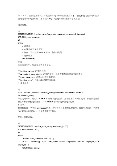
在SQL中,函数是用于执行特定任务并返回结果的数据库对象。
创建和使用函数可以提高查询的效率和可重用性。
下面是在SQL中创建和使用函数的常见用法:创建函数:sqlCREATE FUNCTION function_name (parameter1 datatype, parameter2 datatype)RETURNS return_datatypeASBEGIN--函数体--在这里编写函数逻辑--例如,可以使用SELECT语句、条件语句等--返回结果RETURN result;END;在上述语法中,你需要提供以下信息:* `function_name`:函数的名称。
* `parameter1, parameter2`:函数的参数。
每个参数都需要指定数据类型。
* `return_datatype`:函数返回的数据类型。
* `function_body`:包含函数逻辑的代码块。
2. 使用函数:sqlSELECT column1, column2, function_name(parameter1, parameter2) AS resultFROM table_name;在上述语法中,你可以在SELECT语句中使用函数,并将结果作为列名返回。
你需要将函数的名称和参数传递给函数,并在SELECT语句中选择要返回的列。
3. 示例:假设我们有一个名为employees的表,其中包含员工的姓名和薪水。
我们可以创建一个函数来计算员工的总收入,并在查询中使用它。
首先,创建函数:sqlCREATE FUNCTION calculate_total_salary (employee_id INT)RETURNS DECIMAL(10, 2)ASBEGINDECLARE total_salary DECIMAL(10, 2);SELECT SUM(salary) INTO total_salary FROM employees WHERE employee_id = employee_id;RETURN total_salary;END;然后,在查询中使用该函数:sqlSELECT employee_name, calculate_total_salary(employee_id) AS total_salary FROM employees;。
sql条件函数
sql条件函数
SQL条件函数是用于查询数据时,根据特定条件返回相应的结果集的函数。
常用的条件函数包括:
1. WHERE函数:根据指定的条件筛选出符合条件的数据。
例如,SELECT * FROM table WHERE column1='value';
2. LIKE函数:用于模糊匹配数据。
例如,SELECT * FROM table WHERE column1 LIKE '%value%';
3. IN函数:用于查询符合多个条件中的任意一个条件的数据。
例如,SELECT * FROM table WHERE column1 IN ('value1', 'value2', 'value3');
4. BETWEEN函数:查询介于两个值之间的数据。
例如,SELECT * FROM table WHERE column1 BETWEEN value1 AND value2;
5. EXISTS函数:用于判断查询的子查询是否存在数据。
例如,SELECT * FROM table1 WHERE EXISTS (SELECT * FROM table2 WHERE table1.column1 = table2.column2);
6. NOT函数:用于取反查询结果。
例如,SELECT * FROM table WHERE NOT column1='value';
这些条件函数可以组合使用,以实现更复杂的查询需求。
在实际应用中,需要根据具体的查询需求选择合适的条件函数。
- 1 -。
- 1、下载文档前请自行甄别文档内容的完整性,平台不提供额外的编辑、内容补充、找答案等附加服务。
- 2、"仅部分预览"的文档,不可在线预览部分如存在完整性等问题,可反馈申请退款(可完整预览的文档不适用该条件!)。
- 3、如文档侵犯您的权益,请联系客服反馈,我们会尽快为您处理(人工客服工作时间:9:00-18:30)。
Sturm–Liouville theoryFrom Wikipedia, the free encyclopediaIn mathematics and its applications, a classical Sturm–Liouville equation , named after Jacques Charles François Sturm (1803–1855) and Joseph Liouville (1809–1882), is a real second-order linear differential equation of the formwhere y is a function of the free variable x . Here the functions p (x ) > 0, q (x ), and w (x ) > 0 arespecified at the outset. In the simplest of cases all are continuous on the finite closed interval [a ,b ], and p has continuous derivative . In addition, the function y is typically required to satisfy some boundary conditions at a and b . The function w (x ), which is sometimes called r (x ), is called the "weight" or "density" function.The value of λ is not specified in the equation; finding the values of λ for which there exists a non-trivial solution of (1) satisfying the boundary conditions is part of the problem called the Sturm–Liouville (S L) problem .Such values of λ when they exist are called the eigenvalues of the boundary value problem defined by (1) and the prescribed set of boundary conditions. The corresponding solutions (for such a λ) are the eigenfunctions of this problem. Under normal assumptions on the coefficient functions p (x ), q (x ), and w (x ) above, they induce a Hermitian differential operator in some function space defined by boundary conditions. The resulting theory of the existence and asymptotic behavior of theeigenvalues, the corresponding qualitative theory of the eigenfunctions and their completeness in a suitable function space became known as Sturm–Liouville theory . This theory is important in applied mathematics, where S–L problems occur very commonly, particularly when dealing with linear partial differential equations that are separable.Sturm–Liouville theoryUnder the assumptions that the S–L problem is regular, that is, p (x ), w (x ) > 0, and p (x ), p'(x ), q (x ), and w (x ) are continuous functions over the finite interval [a , b ], with separated boundary conditionsof the form(1)Contents1 Sturm–Liouville theory2 Sturm–Liouville form 2.1 Examples3 Sturm–Liouville equations as self-adjoint differential operators4 Example5 Application to normal modes6 See also7 References(2)wherethe main tenet of Sturm–Liouville theory states that:The eigenvalues λ1, λ2, λ3, ... of the regular Sturm–Liouville problem (1)-(2)-(3) are real and can be ordered such thatCorresponding to each eigenvalue λn is a unique (up to a normalization constant)eigenfunction y n (x ) which has exactly n − 1 zeros in (a , b ). The eigenfunction y n (x ) is called the n -th fundamental solution satisfying the regular Sturm–Liouville problem (1)-(2)-(3).The normalized eigenfunctions form an orthonormal basisin the Hilbert space L 2([a , b ],w (x ) dx ). Here δmn is a Kronecker delta.Note that, unless p (x ) is continuously differentiable and q (x ), w (x ) are continuous, the equation has to be understood in a weak sense.Sturm–Liouville formThe differential equation (1) is said to be in Sturm–Liouville form or self-adjoint form . Allsecond-order linear ordinary differential equations can be recast in the form on the left-hand side of (1) by multiplying both sides of the equation by an appropriate integrating factor (although the same is not true of second-order partial differential equations, or if y is a vector.)ExamplesThe Bessel equation:can be written in Sturm–Liouville form asThe Legendre equation,can easily be put into Sturm–Liouville form, since D (1 − x 2) = −2x, so, the Legendre equation is equivalent to(3)Less simple is such a differential equation asDivide throughout by x 3:Multiplying throughout by an integrating factor ofgiveswhich can be easily put into Sturm–Liouville form sinceso the differential equation is equivalent toIn general, given a differential equationdividing by P (x ), multiplying through by the integrating factorand then collecting gives the Sturm–Liouville form.Sturm–Liouville equations as self-adjoint differential operatorsThe mapcan be viewed as a linear operator mapping a function u to another functionLu. We may study thislinear operator in the context of functional analysis. In fact, equation (1) can be written asThis is precisely the eigenvalue problem; that is, we are trying to find the eigenvalues λ1, λ2, λ3, ... and the corresponding eigenvectors u 1, u 2, u 3, ... of the L operator. The proper setting for this problem is the Hilbert space L 2([a , b ],w (x ) dx ) with scalar productIn this space L is defined on sufficiently smooth functions which satisfy the above boundary conditions. Moreover, L gives rise to a self-adjoint operator. This can be seen formally by using integration by parts twice, where the boundary terms vanish by virtue of the boundary conditions. It then follows that the eigenvalues of a Sturm–Liouville operator are real and that eigenfunctions of L corresponding to different eigenvalues are orthogonal. However, this operator is unbounded and hence existence of an orthonormal basis of eigenfunctions is not evident. To overcome this problem one looks at the resolventwhere z is chosen to be some real number which is not an eigenvalue. Then, computing the resolvent amounts to solving the inhomogeneous equation, which can be done using the variation of parameters formula. This shows that the resolvent is an integral operator with a continuoussymmetric kernel (the Green's function of the problem). As a consequence of the Arzelà–Ascoli theorem this integral operator is compact and existence of a sequence of eigenvalues αn which converge to 0 and eigenfunctions which form an orthonormal basis follows from the spectraltheorem for compact operators. Finally, note that (L − z ) − 1u = αu is equivalent to Lu = (z + α − 1)u . If the interval is unbounded, or if the coefficients have singularities at the boundary points, one calls L singular. In this case the spectrum does no longer consist of eigenvalues alone and can contain a continuous component. There is still an associated eigenfunction expansion (similar to Fourier series versus Fourier transform). This is important in quantum mechanics, since the one-dimensional Schrödinger equation is a special case of a S–L equation.ExampleWe wish to find a function u (x ) which solves the following Sturm–Liouville problem:where the unknowns are λ and u (x ). As above, we must add boundary conditions, we take for exampleObserve that if k is any integer, then the function(4)is a solution with eigenvalue λ = −k 2. We know that the solutions of a S–L problem form an orthogonal basis, and we know from Fourier series that this set of sinusoidal functions is anorthogonal basis. Since orthogonal bases are always maximal (by definition) we conclude that the S–L problem in this case has no other eigenvectors.Given the preceding, let us now solve the inhomogeneous problemwith the same boundary conditions. In this case, we must write f (x ) = x in a Fourier series. The reader may check, either by integrating ∫exp(ikx )x d x or by consulting a table of Fourier transforms, that we thus obtainThis particular Fourier series is troublesome because of its poor convergence properties. It is not clear a priori whether the series converges pointwise. Because of Fourier analysis, since the Fourier coefficients are "square-summable", the Fourier series converges in L 2 which is all we need for this particular theory to function. We mention for the interested reader that in this case we may rely on a result which says that Fourier's series converges at every point of differentiability, and at jump points (the function x , considered as a periodic function, has a jump at π) converges to the average of the left and right limits (see convergence of Fourier series). Therefore, by using formula (4), we obtain that the solution isIn this case, we could have found the answer using antidifferentiation. This technique yields u = (x 3 − π2x )/6, whose Fourier series agrees with the solution we found. The antidifferentiation technique is no longer useful in most cases when the differential equation is in many variables.Application to normal modesSuppose we are interested in the modes of vibration of a thin membrane, held in a rectangular frame, 0 < x < L 1, 0 < y < L 2. We know the equation of motion for the vertical membrane's displacement, W (x , y , t ) is given by the wave equation:The equation is separable (substituting W = X (x ) × Y (y ) × T (t )), and the normal mode solutions that have harmonic time dependence and satisfy the boundary conditions W = 0 at x = 0, L 1 and y = 0, L 2 are given bywhere m and n are non-zero integers, A mn is an arbitrary constant andSince the eigenfunctions W mn form a basis, an arbitrary initial displacement can be decomposed into a sum of these modes, which each vibrate at their individual frequencies ωmn . Infinite sums are also valid, as long as they converge.See alsoNormal modeSelf-adjointReferencesP. Hartman, Ordinary Differential Equations , SIAM, Philadelphia, 2002 (2nd edition). ISBN 978-0-898715-10-1A. D. Polyanin and V. F. Zaitsev, Handbook of Exact Solutions for Ordinary Differential Equations , Chapman & Hall/CRC Press, Boca Raton, 2003 (2nd edition). ISBN 1-58488-297-2G. Teschl, Ordinary Differential Equations and Dynamical Systems , http://www.mat.univie.ac.at/~gerald/ftp/book-ode/ (Chapter 5)G. Teschl, Mathematical Methods in Quantum Mechanics and Applications to Schrödinger Operators , http://www.mat.univie.ac.at/~gerald/ftp/book-schroe/ (see Chapter 9 for singular S-L operators and connections with quantum mechanics)A. Zettl, Sturm–Liouville Theory , American Mathematical Society, 2005. ISBN 0-8218-3905-5.Retrieved from "/wiki/SturmâLiouville_theory" Categories: Ordinary differential equations | Operator theory | Spectral theoryThis page was last modified on 29 August 2010 at 21:35.Text is available under the Creative Commons Attribution-ShareAlike License; additional terms may apply. See Terms of Use for details.Wikipedia® is a registered trademark of the Wikimedia Foundation, Inc., a non-profit organization. Privacy policy About WikipediaDisclaimers。