ABAQUS用户子程序
ABAQUS子程序

Home浅谈ABAQUS用户子程序李青清华大学工程力学系摘要本文首先概要介绍了ABAQUS的用户子程序和应用程序,然后从参数,功能两方面详细论述了DLOAD, UEXTERNALDB, URDFIL三个用户子程序和GETENVVAR,POSFIL,DBFILE三个应用程序,并详细介绍了ABAQUS的结果文件(.FIL)存储格式。
关键字ABAQUS,用户子程序,应用程序,结果文件一、前言:ABAQUS为用户提供了强大而又灵活的用户子程序接口(USER SUBROUTINE)和应用程序接口(UTILITY ROUTINE)。
ABAQUS 6.2.5一共有42个用户子程序接口,13个应用程序接口,用户可以定义包括边界条件、荷载条件、接触条件、材料特性以及利用用户子程序和其它应用软件进行数据交换等等。
这些用户子程序接口使用户解决一些问题时有很大的灵活性,同时大大的扩充了ABAQUS的功能。
例如:如果荷载条件是时间的函数,这在ABAQUS/CAE 和INPUT 文件中是难以实现的,但在用户子程序DLOAD中就很容易实现。
二.在ABAQUS中使用用户子程序ABAQUS的用户子程序是根据ABAQUS提供的相应接口,按照FORTRAN语法用户自己编写的代码。
在一个算例中,用户可以用到多个用户子程序,但必须把它们放在一个以.FOR为扩展名的文件中。
运行带有用户子程序的算例时有两种方法,一是在CAE中运行,在EDIT JOB菜单的GENERAL子菜单的USER SUBROUTINE FILE对话框中选择用户子程序所在的文件即可;另外是在ABABQUS COMMAND用运行,语法如下:ABAQUS JOB=[JOB] USER¡[.FOR]¡C用户在编写用户子程序时,要注意以下几点:1.用户子程序不能嵌套。
即任何用户子程序都不能调用任何其他用户子程Home序,但可以调用用户自己编写的FORTRAN子程序和ABAQUS应用程序。
Abaqus 用户子程序uinter介绍
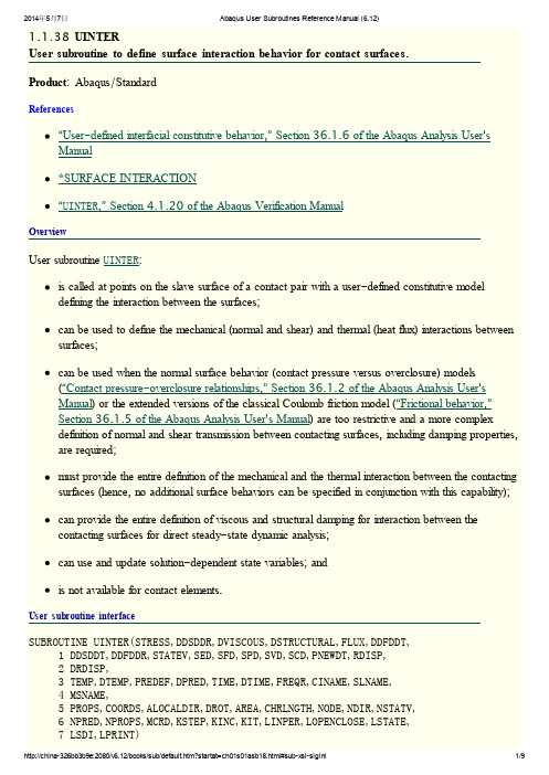
1.1.38 UINTERUser subroutine to define surface interaction behavior for contact surfaces.Product: Abaqus/StandardReferences“User-defined interfacial constitutive behavior,” Section 36.1.6 of the Abaqus Analysis User'sManual*SURFACE INTERACTION“U I N T E R,” Section 4.1.20 of the Abaqus Verification ManualOverviewUser subroutine U I N T E R:is called at points on the slave surface of a contact pair with a user-defined constitutive modeldefining the interaction between the surfaces;can be used to define the mechanical (normal and shear) and thermal (heat flux) interactions between surfaces;can be used when the normal surface behavior (contact pressure versus overclosure) models(“Contact pressure-overclosure relationships,” Section 36.1.2 of the Abaqus Analysis User'sManual) or the extended versions of the classical Coulomb friction model (“Frictional behavior,”Section 36.1.5 of the Abaqus Analysis User's Manual) are too restrictive and a more complexdefinition of normal and shear transmission between contacting surfaces, including damping properties, are required;must provide the entire definition of the mechanical and the thermal interaction between the contacting surfaces (hence, no additional surface behaviors can be specified in conjunction with this capability);can provide the entire definition of viscous and structural damping for interaction between thecontacting surfaces for direct steady-state dynamic analysis;can use and update solution-dependent state variables; andis not available for contact elements.User subroutine interfaceS U B R O U T I N E U I N T E R(S T R E S S,D D S D D R,D V I S C O U S,D S T R U C T U R A L,F L U X,D D F D D T,1D D S D D T,D D F D D R,S T A T E V,S E D,S F D,S P D,S V D,S C D,P N E W D T,R D I S P,2D R D I S P,3T E M P,D T E M P,P R E D E F,D P R E D,T I M E,D T I M E,F R E Q R,C I N A M E,S L N A M E,4M S N A M E,5P R O P S,C O O R D S,A L O C A L D I R,D R O T,A R E A,C H R L N G T H,N O D E,N D I R,N S T A T V,6N P R E D,N P R O P S,M C R D,K S T E P,K I N C,K I T,L I N P E R,L O P E N C L O S E,L S T A T E,7L S D I,L P R I N T)CI N C L U D E'A B A_P A R A M.I N C'CC H A R A C T E R*80C I N A M E,S L N A M E,M S N A M ED I ME N S I O N S T R E S S(N D I R),D D S D D R(N D I R,N D I R),F L U X(2),D D F D D T(2,2),1D D S D D T(N D I R,2),D D F D D R(2,N D I R),S T A T E V(N S T A T V),2R D I S P(N D I R),D R D I S P(N D I R),T E M P(2),D T E M P(2),P R E D E F(2,N P R E D),3D P R E D(2,N P R E D),T I M E(2),P R O P S(N P R O P S),C O O R D S(M C R D),4A L O C A L D I R(3,3),D R O T(2,2),D V I S C O U S(N D I R,N D I R),5D S T R U C T U R A L(N D I R,N D I R)user coding to define S T R E S S,D D S D D R,F L U X,D D F D D T,D D S D D T,D D F D D R,and, optionally,S T A T E V,S E D,S F D,S P D,S V D,S C D,P N E W D T,L O P E N C L O S E,L S T A T E,L S D I,D V I S C O U S,D S T R U C T U R A LR E T U R NE N DVariables to be definedS T R E S S(N D I R)This array is passed in as the stress between the slave and master surfaces at the beginning of theincrement and must be updated in this routine to be the stress at the end of the increment. The stress must be defined in a local coordinate system (see A L O C D I R). This variable must be defined for astress/displacement, a fully coupled temperature-displacement, or a coupled thermal-electrical-structural analysis. The sign convention for stresses is that a positive stress indicates compression across contact surfaces, while a negative stress indicates tension.D D S D D R(N D I R,N D I R)Interface stiffness matrix. D D S D D R(I,J)defines the change in the Ith stress component at the end of the time increment caused by an infinitesimal perturbation of the Jth component of the relativedisplacement increment array. Unless you invoke the unsymmetric equation solution capability in the contact property model definition (“Use with the unsymmetric equation solver in Abaqus/Standard” in “User-defined interfacial constitutive behavior,” Section 36.1.6 of the Abaqus Analysis User'sManual), Abaqus/Standard will use only the symmetric part of D D S D D R. For a particular off-diagonal (I,J) entry, the symmetrization is done by halving the sum of (I,J) and (J,I) components. D D S D D R must be defined for a stress/displacement, a fully coupled temperature-displacement, or a coupled thermal-electrical-structural analysis to ensure proper convergence characteristics.F L U X(2)Magnitude of the heat flux flowing into the slave and master surfaces, respectively. This array is passed in as the value at the beginning of the increment and must be updated to the flux at the end of theincrement. The convention for defining the flux is that a positive flux indicates heat flowing into asurface, while a negative flux indicates heat flowing out of the surface. This variable must be defined fora heat transfer, a fully coupled temperature-displacement, or a coupled thermal-electrical-structuralanalysis. The sum of these two flux terms represents the heat generated in the interface, and thedifference in these flux terms represents the heat conducted through the interface.D D F D D T(2,2)The negative of the variation of the flux at the two surfaces with respect to their respectivetemperatures, for a fixed relative displacement. This variable must be defined for a heat transfer, a fully coupled temperature-displacement, or a coupled thermal-electrical-structural analysis to ensure proper convergence characteristics. The entries in the first row contain the negatives of the derivatives ofF L U X(1)with respect to T E M P(1)and T E M P(2), respectively. The entries in the second row containthe negatives of the corresponding derivatives of F L U X(2).D D S D D T(N D I R,2)Variation of the stress with respect to the temperatures of the two surfaces for a fixed relativedisplacement. This variable is required only for thermally coupled elements (in a fully coupledtemperature-displacement or a coupled thermal-electrical-structural analysis), in which the stress is a function of the surface temperatures. D D S D D T(N D I R,1)corresponds to the slave surface, andD D S D D T(N D I R,2)corresponds to the master surface.D D F D D R(2,N D I R)Variation of the flux with respect to the relative displacement between the two surfaces. This variable is required only for thermally coupled elements (in a fully coupled temperature-displacement or a coupled thermal-electrical-structural analysis), in which the flux is a function of the relative displacement.D D F D D R(1,N D I R)corresponds to the slave surface, and D D F D D R(2,N D I R)corresponds to the mastersurface.Variables that can be updatedD V I S C O U S(N D I R,N D I R)Interface viscous damping matrix that can be used only in direct steady-state dynamic analysis.D V I S C O U S(I,J)defines an element in the material viscous damping matrix at the current frequency.Abaqus/Standard requires that this element is defined as a damping value for each of the (I, J) entries times the current frequency value F R E Q R obtained from the argument list.Unless you invoke the unsymmetric equation solution capability in the contact property model definition (“Use with the unsymmetric equation solver in Abaqus/Standard” in “User-defined interfacialconstitutive behavior,” Section 36.1.6 of the Abaqus Analysis User's Manual), Abaqus/Standard uses only the symmetric part of D V I S C O U S. For a particular off-diagonal (I, J) entry the symmetrization is done by halving the sum of the (I, J) and (J, I) components.D S T R U C T U R A L(N D I R,N D I R)Interface structural damping matrix that can be used only in direct steady-state dynamic analysis.D S T R U C T U R A L(I,J)defines an element in the material structural damping matrix.Unless you invoke the unsymmetric equation solution capability in the contact property model definition(“Use with the unsymmetric equation solver in Abaqus/Standard” in “User-defined interfacialconstitutive behavior,” Section 36.1.6 of the Abaqus Analysis User's Manual), Abaqus/Standard uses only the symmetric part of D S T R U C T U R A L. For a particular off-diagonal (I, J) entry the symmetrization is done by halving the sum of the (I, J) and (J, I) components.S T A T E V(N S T A T V)An array containing the solution-dependent state variables. These are passed in as values at thebeginning of the increment and must be returned as values at the end of the increment. You define the number of available state variables as described in“Allocating space” in “User subroutines: overview,”Section 18.1.1 of the Abaqus Analysis User's Manual.S E DThis variable is passed in as the value of the elastic energy density at the start of the increment and should be updated to the elastic energy density at the end of the increment. This variable is used for output only and has no effect on other solution variables. It contributes to the output variable ALLSE. S F DThis variable should be defined as the incremental frictional dissipation. The units are energy per unit area. This variable is used for output only and has no effect on other solution variables. It contributes to the output variables ALLFD and SFDR (and related variables). For computing its contribution toSFDR, S F D is divided by the time increment.S P DThis variable should be defined as the incremental dissipation due to plasticity effects in the interfacial constitutive behavior. The units are energy per unit area. This variable is used for output only and has no effect on other solution variables. It contributes to the output variable ALLPD.S V DThis variable should be defined as the incremental dissipation due to viscous effects in the interfacial constitutive behavior. The units are energy per unit area. This variable is used for output only and has no effect on other solution variables. It contributes to the output variable ALLVD.S C DThis variable should be defined as the incremental dissipation due to creep effects in the interfacialconstitutive behavior. The units are energy per unit area. This variable is used for output only and has no effect on other solution variables. It contributes to the output variable ALLCD.P N E W D TRatio of suggested new time increment to the time increment currently being used (D T I M E, see below).This variable allows you to provide input to the automatic time incrementation algorithms inAbaqus/Standard (if automatic time incrementation is chosen).P N E W D T is set to a large value before each call to U I N T E R.If P N E W D T is redefined to be less than 1.0, Abaqus/Standard must abandon the time increment and attempt it again with a smaller time increment. The suggested new time increment provided to theautomatic time integration algorithms is P N E W D T × D T I M E, where the P N E W D T used is the minimum value for all calls to user subroutines that allow redefinition of P N E W D T for this iteration.If P N E W D T is given a value that is greater than 1.0 for all calls to user subroutines for this iteration and the increment converges in this iteration, Abaqus/Standard may increase the time increment. Thesuggested new time increment provided to the automatic time integration algorithms is P N E W D T ×D T I M E, where the P NE W D T used is the minimum value for all calls to user subroutines for this iteration.If automatic time incrementation is not selected in the analysis procedure, values of P N E W D T greater than1.0 will be ignored and values of P N E W D T less than 1.0 will cause the job to terminate.L O P E N C L O S EAn integer flag that is used to track the contact status in situations where user subroutine U I N T E R is used to model standard contact between two surfaces, like the default hard contact model inAbaqus/Standard. It comes in as the value at the beginning of the current iteration and should be set to the value at the end of the current iteration. It is set to –1 at the beginning of the analysis beforeU I N T E R is called. You should set it to 0 to indicate an open status and to 1 to indicate a closed status.A change in this flag from one iteration to the next will have two effects. It will result in output relatedto a change in contact status if you request a detailed contact printout in the message file (“TheAbaqus/Standard message file” in “Output,” Section 4.1.1 of the Abaqus Analysis User's Manual). In addition, it will also trigger a severe discontinuity iteration. Any time this flag is reset to a value of –1, Abaqus/Standard assumes that the flag is not being used. A change in this flag from –1 to another value or vice versa will not have any of the above effects.L S T A T EAn integer flag that should be used in non-standard contact situations where a simple open/close status is not appropriate or enough to describe the state. It comes in as the value at the beginning of thecurrent iteration and should be set to the value at the end of the current iteration. It is set to –1 at the beginning of the analysis before U I N T E R is called. It can be assigned any user-defined integer value, each corresponding to a different state. You can track changes in the value of this flag and use it to output appropriate diagnostic messages to the message file (unit 7). You may choose to outputdiagnostic messages only when a detailed contact printout is requested (“The Abaqus/Standardmessage file” in “Output,” Section 4.1.1 of the Abaqus Analysis User's Manual). In the latter case, the L P R I N T parameter is useful. In conjunction with the L S T A T E flag, you may also utilize the L S D I flag to trigger a severe discontinuity iteration any time the state changes from one iteration to the next. Any time this flag is reset to a value of –1, Abaqus/Standard assumes that the flag is not being used.L S D IThis flag is set to 0 before each call to U I N T E R and should be set to 1 if the current iteration should be treated as a severe discontinuity iteration. This would typically be done in non-standard contactsituations based on a change in the value of the L S T A T E flag from one iteration to the next. The use of this flag has no effect when the L O P E N C L O S E flag is also used. In that case, severe discontinuityiterations are determined based on changes in the value of L O P E N C L O S E alone.Variables passed in for informationR D I S P(N D I R)An array containing the current relative positions between the two surfaces at the end of the increment.The first component is the relative position of the point on the slave surface, with respect to the master surface, in the normal direction. The second and third components, if applicable, are the accumulated incremental relative tangential displacements, measured from the beginning of the analysis. For therelative position in the normal direction a negative quantity represents an open status, while a positive quantity indicates penetration into the master surface. For open points on the slave surface for which no pairing master is found, the first component is a very large negative number (–1 × 1036). The local directions in which the relative displacements are defined are stored in A L O C A L D I R.D R D I S P(N D I R)An array containing the increments in relative positions between the two surfaces.T E M P(2)Temperature at the end of the increment at a point on the slave surface and the opposing mastersurface, respectively.D TE M P(2)Increment in temperature at the point on the slave surface and the opposing master surface,respectively.P R E D E F(2,N P R E D)An array containing pairs of values of all the predefined field variables at the end of the currentincrement (initial values at the beginning of the analysis and current values during the analysis). The first value in a pair, P R E D E F(1,N P R E D), corresponds to the value at the point on the slave surface, and the second value, P F R E D E F(2,N P R E D), corresponds to the value of the field variable at the nearest point on the opposing surface.D P RE D(2,N P R E D)Array of increments in predefined field variables.T I M E(1)Value of step time at the end of the increment.T I M E(2)Value of total time at the end of the increment.D T I M ECurrent increment in time.F R E Q RCurrent frequency for direct steady-state dynamic analysis in rad/time.C I N A M EUser-specified surface interaction name, left justified.S L N A M ESlave surface name.M S N A M EMaster surface name.P R O P S(N P R O P S)User-specified array of property values to define the interfacial constitutive behavior between thecontacting surfaces.C O O RD S(M C R D)An array containing the current coordinates of this point.A L O C A L D I R(3,3)An array containing the direction cosines of the local surface coordinate system. The directions are stored in columns. For example, A L O C A L D I R(1,1), A L O C A L D I R(2,1), and A L O C A L D I R(3,1)give the (1, 2, 3) components of the normal direction. Thus, the first direction is the normal direction to the surface, and the remaining two directions are the slip directions in the plane of the surface. The local system is defined by the geometry of the master surface. The convention for the local directions is the same as the convention in situations where the model uses the built-in contact capabilities inAbaqus/Standard (described in“Contact formulations in Abaqus/Standard,” Section 37.1.1 of the Abaqus Analysis User's Manual, for the tangential directions).D R O T(2,2)Rotation increment matrix. For contact with a three-dimensional rigid surface, this matrix represents the incremental rotation of the surface directions relative to the rigid surface. It is provided so that vector-or tensor-valued state variables can be rotated appropriately in this subroutine. Relative displacement components are already rotated by this amount before U I N T E R is called. This matrix is passed in as a unit matrix for two-dimensional and axisymmetric contact problems.A R E ASurface area associated with the contact point.C H R L N G T HCharacteristic contact surface face dimension.N O D EUser-defined global slave node number (or internal node number for models defined in terms of an assembly of part instances) involved with this contact point. Corresponds to the predominant slave node of the constraint if the surface-to-surface contact formulation is used.N D I RNumber of force components at this point.N S T A T VNumber of solution-dependent state variables.N P R E DNumber of predefined field variables.N P R O P SUser-defined number of property values associated with this interfacial constitutive model (“Interfacial constants” in “User-defined interfacial constitutive behavior,” Section 36.1.6 of the Abaqus Analysis User's Manual).M C R DNumber of coordinate directions at the contact point.K S T E PStep number.K I N CIncrement number.K I TIteration number. K I T=0 for the first assembly, K I T=1 for the first recovery/second assembly,K I T=2 for the second recovery/third assembly, and so on.L I N P E RLinear perturbation flag. L I N P E R=1 if the step is a linear perturbation step. L I N P E R=0 if the step is a general step. For a linear perturbation step, the inputs to user subroutine U I N T E R represent perturbation quantities about the base state. The user-defined quantities in U I N T E R are also perturbation quantities.The Jacobian terms should be based on the base state. No change in contact status should occurduring a linear perturbation step.L P R I N TThis flag is equal to 1 if a detailed contact printout to the message file is requested and 0 otherwise (“The Abaqus/Standard message file” in “Output,” Section 4.1.1 of the Abaqus Analysis User'sManual). This flag can be used to print out diagnostic messages regarding changes in contact statusselectively only when a detailed contact printout is requested.。
UEL

ABAQUS 6.1版本发布会暨99中国地区用户会议
编程要求
单元采用数值积分;因此,需要在UEL中 定义下面的量: 单元[B]矩阵,用于联系轴向应变、曲 率与单元位移{ue}:
Bue
本构律矩阵[D],用于联系轴向力F、 弯矩M与轴向应变、曲率 :
*USER ELEMENT, TYPE=Un, NODES=, COORDINATES=, PROPERTIES=, I PROPERTIES=, VARIABLES=, UNSYMM Data lines(s) *ELEMENT,TYPE=Un, ELSET=UEL Data line(s) *UEL PROPERTY,ELSET=UEL Data line(s) *USER SUBROUTINE, (INPUT=file_name)
清华大学工程力学系
ABAQUS 6.1版本发布会暨99中国地区用户会议
编写和测试UEL
编写ABAQUS用户子程序的基本规则: 遵从FORTRAN 77或C的语法。 确保所有的变量都定义和初始化过。 为状态变量分配足够的存储空间。 ABAQUS 5.8-10版本要求FORTRAN编译器 的版本为5.0;从ABAQUS 5.8-14开始, 要求FORTRAN编译器的版本为6.0。
分析中定义接触面或节点之间的热传导系数 的用户子程序
清华大学工程力学系
ABAQUS 6.1版本发布会暨99中国地区用户会议
GAPELECTR-在热-电耦合分析中定义
表面间导电系数的用户子程序
HARDINI-定义初始等效塑性应变和初
始背应力张量的用户子程序
HETVAL-在热传导分析中定义内部热
SIGINI-定义初应力场的用户子程序
完整word版ABAQUS中Fortran子程序调用方法—自己总结
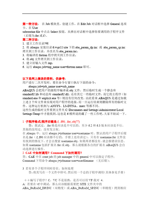
第一种方法:在Job模块里,创建工作,在Edit Job对话框中选择General选项卡,在Usersubroutine file中点击Select按钮,从弹出对话框中选择你要调用的子程序文件(后缀为.for或.f)。
第二种方法:1. 建立工作目录?崠2. 将Abaqus安装目录\6.4-pr11\site下的aba_param_dp.inc 或aba_param_sp.inc 拷贝到工作目录,并改名为aba_param.inc;3. 将编译的fortran程序拷贝到工作目录;4.将.obj文件拷贝到工作目录;5. 建立好输入文件.inp;6. 运行abaqus job=inp_name user=fortran name即可。
以下是网上摘录的资料,供参考:用户进行二次开发时,要在命令行窗口执行下面的命令:abaqus job=job_name user=sub_nameABAQUS会把用户的源程序编译成obj文件,然后临时生成一个静态库standardU.lib和动态库standardU.dll,还有其它一些临时文件,而它的主程序(如standard.exe和explicit.exe等)则没有任何改变,由此看来ABAQUS是通过加载上述2个库文件来实现对用户程序的连接,而一旦运行结束则删除所有的临时文件。
这种运行机制与ANSYS、LS-DYNA、marc等都不同。
这些生成的临时文件要到文件夹C:\Documents and Settings\Administrator\Local Settings\Temp\中才能找到,这也是6楼所说的藏了一些工作吧,大家不妨试一下。
1子程序格式(程序后缀是.f; .f90; .for;.obj??)答:我试过,.for格是应该是不可以的,至少6.2和6.3版本应该是不行,其他的没用过,没有发言权。
在Abaqus中,运行abaqus j=jobname user=username时,默认的用户子程序后缀名是.for(.f,.f90应该都不行的,手册上也有讲过),只有在username.for文件没有找到的情况下,才会去搜索username.obj,如果两者都没有,就会报错误信息。
abaqus 子程序 简单案例

abaqus 子程序简单案例1. 案例一:ABAQUS子程序在计算机辅助工程中的应用在计算机辅助工程中,ABAQUS子程序是一种被广泛应用的工具,用于求解各种复杂的物理问题。
它可以在ABAQUS有限元软件中调用,通过编写用户自定义的子程序来实现特定的功能。
下面将介绍一些常见的ABAQUS子程序案例。
2. 案例二:ABAQUS子程序在材料力学中的应用ABAQUS子程序在材料力学中的应用非常广泛。
例如,可以通过自定义的子程序来模拟材料的非线性行为、塑性变形、断裂行为等。
通过在子程序中编写相应的材料本构模型和损伤模型,可以准确地预测材料的力学性能。
3. 案例三:ABAQUS子程序在流体力学中的应用ABAQUS子程序在流体力学中也有重要的应用。
例如,可以通过自定义的子程序来模拟流体的非牛顿性、多相流动、湍流等现象。
通过在子程序中编写相应的流体本构模型和湍流模型,可以准确地模拟流体的流动行为。
4. 案例四:ABAQUS子程序在结构力学中的应用ABAQUS子程序在结构力学中也非常有用。
例如,可以通过自定义的子程序来模拟结构的非线性行为、接触和摩擦、动力响应等。
通过在子程序中编写相应的结构本构模型和接触模型,可以准确地预测结构的力学性能。
5. 案例五:ABAQUS子程序在热传导中的应用ABAQUS子程序在热传导中的应用也非常广泛。
例如,可以通过自定义的子程序来模拟材料的热传导行为、热辐射、相变等。
通过在子程序中编写相应的热传导模型和相变模型,可以准确地预测材料的热学性能。
6. 案例六:ABAQUS子程序在电磁场中的应用ABAQUS子程序在电磁场中的应用也有一定的研究价值。
例如,可以通过自定义的子程序来模拟电磁场的非线性行为、磁饱和、电磁感应等。
通过在子程序中编写相应的电磁场模型和电磁感应模型,可以准确地模拟电磁场的行为。
7. 案例七:ABAQUS子程序在声学中的应用ABAQUS子程序在声学领域中也有一定的应用。
abaqus子程序实例
abaqus子程序实例
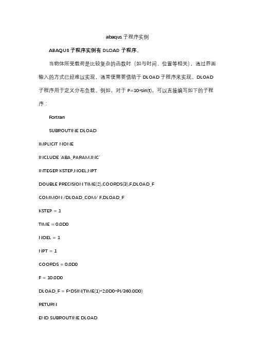
ABAQUS子程序实例有DLOAD子程序。
当物体所受载荷是比较复杂的函数时(如与时间、位置等相关),通过界面输入的方式已经难以实现,通常便需要借助于DLOAD子程序来实现。
DLOAD 子程序用于定义分布负载。
例如,对于P=10*sin(t),可以直接编写如下的子程序:
Fortran
SUBROUTINE DLOAD
IMPLICIT NONE
INCLUDE 'ABA_PARAM.INC'
INTEGER KSTEP,NOEL,NPT
DOUBLE PRECISION TIME(2),COORDS(3),F,DLOAD_F
COMMON /DLOAD_COM/ F,DLOAD_F
KSTEP = 1
TIME = 0.0D0
NOEL = 1
NPT = 1
COORDS = 0.0D0
F = 10.0D0
DLOAD_F = F*DSIN(TIME(1)*2.0D0*PI/360.0D0)
RETURN
END SUBROUTINE DLOAD
上述程序中,已经明确指出user coding to define F,即表示需要用户自己去定义变量F的值,F的值便表示所加载的载荷大小。
该数值的正负符号有明确的物理意义,对于压力,正数表示压力,负数表示拉力。
也就是说只有F这个变量需要我们去定义,其它的一些变量都是输入变量,是软件传递给我们去使用的,不需要我们去定义。
ABAQUS_Standard用户材料子程序实例

ABAQUS/Standard 用户材料子程序实例-Johnson-Cook 金属本构模型卢剑锋 庄茁* 张帆清华大学工程力学系 北京 100084摘要:用户材料子程序是ABAQUS 提供给用户定义自己的材料属性的Fortran 程序接口,使用户能使用ABAQUS 材料库中没有定义的材料模型。
ABAQUS 中自有的Johnson-Cook 模型只能应用于显式ABAQUS/Explicit 程序中,而我们希望能在隐式ABAQUS/Standard 程序中更精确的实现本构积分,而且应用Johnson-Cook 模型的修正形式。
这就需要通过ABAQUS/Standard 的用户材料子程序UMAT 编程实现。
在UMAT 编程中使用了率相关塑性理论以及完全隐式的应力更新算法。
1 Johnson-Cook 强化模型简介Johnson-Cook (JC )模型用来模拟高应变率下的金属材料。
JC 强化模型表示为三项的乘积,分别反映了应变硬化,应变率硬化和温度软化。
这里使用JC 模型的修正形式:()()*01ln 11n mA B C T εσεε=+++−&& 并使参考应变率01ε=&,这样公式中的A 即为材料的静态屈服应力。
公式中包含,,,,A B n C m 五个参数,需要通过实验来确定。
2 ABAQUS 用户材料子程序用户材料子程序(User-defined Material Mechanical Behavior ,简称UMAT )通过与ABAQUS 主求解程序的接口实现与ABAQUS 的数据交流。
在输入文件中,使用关键字“*USER MATERIAL”表示定义用户材料属性。
子程序概况与接口UMAT 子程序具有强大的功能,使用UMAT 子程序:(1) 可以定义材料的本构关系,使用ABAQUS 材料库中没有包含的材料进行计算,扩充程序功能。
(2)几乎可以用于力学行为分析的任何分析过程,几乎可以把用户材料属性赋予ABAQUS中的任何单元;(3)必须在UMAT中提供材料本构模型的雅可比(Jacobian)矩阵,即应力增量对应变增量的变化率。
abaqus 子程序中coord程序的用法
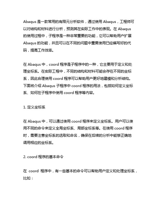
Abaqus是一款常用的有限元分析软件,通过使用Abaqus,工程师可以对结构和材料进行分析,预测其在实际工作中的表现。
在Abaqus的使用过程中,子程序是一种非常重要的功能,它可以帮助用户扩展Abaqus的功能,并且可以在不同的问题中重复使用已经编写好的代码,提高工作效率。
在Abaqus中,coord程序是子程序中的一种,它主要用于定义和处理坐标系。
在实际工程中,不同的结构和材料可能会存在不同的坐标系,因此合理使用coord程序可以帮助用户更好地建模和分析结构。
下面将介绍Abaqus子程序中coord程序的用法,包括如何定义坐标系、如何在子程序中使用coord程序等内容。
1. 定义坐标系在Abaqus中,可以通过使用coord程序来定义坐标系。
用户可以使用不同的命令来定义全局坐标系、局部坐标系等。
在使用coord程序时,需要注意坐标系的选取和命名,确保在后续的分析中能够正确地调用相应的坐标系。
2. coord程序的基本命令在coord程序中,有一些基本的命令可以帮助用户定义和处理坐标系,比如:- `Csys`: 定义坐标系的命令,可以用于定义全局坐标系、局部坐标系等。
- `Transform`: 用于坐标变换,可以将一些特定的坐标系转换到其他坐标系中。
- `Ang`: 定义角度,可以用于在坐标系中定义一些特定的角度。
通过合理地使用这些命令,用户可以很好地定义和处理坐标系,为后续的分析奠定基础。
3. 在子程序中使用coord程序除了在Abaqus的交互式界面中使用coord程序外,用户还可以在子程序中使用coord程序来定义和处理坐标系。
在实际工程中,很多情况下需要重复使用一些特定的坐标系,此时可以将这些操作封装在子程序中,方便在不同的问题中重复使用。
为了在子程序中使用coord程序,用户需要加入一些特定的命令,并且需要注意在子程序中正确地调用和处理坐标系,确保在后续的分析中能够得到正确的结果。
- 1、下载文档前请自行甄别文档内容的完整性,平台不提供额外的编辑、内容补充、找答案等附加服务。
- 2、"仅部分预览"的文档,不可在线预览部分如存在完整性等问题,可反馈申请退款(可完整预览的文档不适用该条件!)。
- 3、如文档侵犯您的权益,请联系客服反馈,我们会尽快为您处理(人工客服工作时间:9:00-18:30)。
当用到某个用户子程序时,用户所关心的主要有两方面:一是ABAQUS提供的用户子程序的接口参数。
有些参数是ABAQUS传到用户子程序中的,例如SUBROUTINE DLOAD中的KSTEP,KINC,COORDS;有些是需要用户自己定义的,例如F。
二是ABAQUS何时调用该用户子程序,对于不同的用户子程序ABAQUS调用的时间是不同的。
有些是在每个STEP的开始,有的是STEP结尾,有的是在每个INCREMENT的开始等等。
当ABAQUS 调用用户子程序是,都会把当前的STEP和INCREMENT利用用户子程序的两个实参KSTEP和KINC传给用户子程序,用户可编个小程序把它们输出到外部文件中,这样对ABAQUS何时调用该用户子程序就会有更深的了解。
(子程序中很重要的就是要知道由abaqus提供的那些参量的意义,如下)首先介绍几个子程序:一.SUBROUTINE DLOAD(F,KSTEP,KINC,TIME,NOEL,NPT,LAYER,KSPT,COORDS, JLTYP,SNAME)参数:1.F为用户定义的是每个积分点所作用的荷载的大小;2.KSTEP,KINC为ABAQUS传到用户子程序当前的STEP和INCREMENT值;3.TIME(1),TIME(2)为当前STEP TIME和INCREMENT TIME的值;4.NOEL,NPT为积分点所在单元的编号和积分点的编号;5.COORDS为当前积分点的坐标;6.除F外,所有参数的值都是ABAQUS传到用户子程序中的。
功能:1.荷载可以被定义为积分点坐标、时间、单元编号和单元节点编号的函数。
2.用户可以从其他程序的结果文件中进行相关操作来定义积分点F的大小。
例1:这个例子在每个积分点施加的荷载不仅是坐标的函数,而且是随STEP变化而变化的。
SUBROUTINE DLOAD(P,KSTEP,KINC,TIME,NOEL,NPT,LAYER,KSPT,COORDS,1 JLTYP,SNAME)INCLUDE 'ABA_PARAM.INC' CDIMENSION TIME(2),COORDS(3)CHARACTER*80 SNAMEPARAMETER (PLOAD=100.E4)IF (KSTEP.EQ.1) THEN !当STEP=1时的荷载大小P=PLOADELSE IF (KSTEP.EQ.2) THEN !当STEP=2时的荷载大小P=COORDS(1)*PLOAD !施加在积分点的荷载P是坐标的函数ELSE IF (KSTEP.EQ.3) THEN !当STEP=3时的荷载大小P=COORDS(1)**2*PLOADELSE IF (KSTEP.EQ.4) THEN !当STEP=4时的荷载大小P=COORDS(1)**3*PLOADELSE IF (KSTEP.EQ.5) THEN !当STEP=5时的荷载大小P=COORDS(1)**4*PLOADEND IFRETURNENDUMAT 子程序具有强大的功能,使用UMAT 子程序:(1) 可以定义材料的本构关系,使用ABAQUS 材料库中没有包含的材料进行计算,扩充程序功能。
(2) 几乎可以用于力学行为分析的任何分析过程,几乎可以把用户材料属性赋予ABAQUS 中的任何单元;(3) 必须在UMAT 中提供材料本构模型的雅可比(Jacobian)矩阵,即应力增量对应变增量的变化率。
(4) 可以和用户子程序“USDFLD”联合使用,通过“USDFLD”重新定义单元每一物质点上传递到UMAT 中场变量的数值。
由于主程序与UMAT 之间存在数据传递,甚至共用一些变量,因此必须遵守有关UMAT 的书写格式,UMAT 中常用的变量在文件开头予以定义,通常格式为:SUBROUTINE UMAT(STRESS,STATEV,DDSDDE,SSE,SPD,SCD,1 RPL,DDSDDT,DRPLDE,DRPLDT,2 STRAN,DSTRAN,TIME,DTIME,TEMP,DTEMP,PREDEF,DPRED,CMNAME,3 NDI,NSHR,NTENS,NSTATV,PROPS,NPROPS,COORDS,DROT,PNEWDT,4 CELENT,DFGRD0,DFGRD1,NOEL,NPT,LAYER,KSPT,KSTEP,KINC)INCLUDE 'ABA_PARAM.INC'CHARACTER*80 CMNAMEDIMENSION STRESS(NTENS),STATEV(NSTATV),1 DDSDDE(NTENS,NTENS),DDSDDT(NTENS),DRPLDE(NTENS),2 STRAN(NTENS),DSTRAN(NTENS),TIME(2),PREDEF(1),DPRED(1),3 PROPS(NPROPS),COORDS(3),DROT(3,3),DFGRD0(3,3),DFGRD1(3,3)user coding to define DDSDDE, STRESS, STATEV, SSE, SPD, SCDand, if necessary, RPL, DDSDDT, DRPLDE, DRPLDT, PNEWDTRETURNENDUMAT 中的应力矩阵、应变矩阵以及矩阵DDSDDE ,DDSDDT ,DRPLDE 等,都是直接分量存储在前,剪切分量存储在后。
直接分量有NDI 个,剪切分量有NSHR 个。
各分量之间的顺序根据单元自由度的不同有一些差异,所以编写UMAT 时要考虑到所使用单元的类别。
下面对UMAT 中用到的一些变量进行说明:DDSDDE(NTENS,NTENS)是一个NTENS 维的方阵,称作雅可比矩阵,,是应力的增量,是应变的增量,DDSDDE(I,J)表示增量步结束时第J 个应变分量的改变引起的第I 个应力分量的变化。
通常雅可比是一个对称矩阵,除非在“*USER MATERIAL”语句中加入了“UNSYMM”参数。
STRESS (NTENS)应力张量矩阵,对应NDI 个直接分量和NSHR 个剪切分量。
在增量步的开始,应力张量矩阵中的数值通过UMAT 和主程序之间的接口传递到UMAT 中,在增量步的结束UMAT 将对应力张量矩阵更新。
对于包含刚体转动的有限应变问题,一个增量步调用UMAT 之前就已经对应力张量的进行了刚体转动,因此在UMAT 中只需处理应力张量的共旋部分。
UMAT 中应力张量的度量为柯西(真实)应力。
STATEV (NSTATEV)用于存储状态变量的矩阵,在增量步开始时将数值传递到UMAT 中。
也可在子程序USDFLD或UEXPAN 中先更新数据,然后增量步开始时将更新后的数据传递到UMAT 中。
在增量步的结束必须更新状态变量矩阵中的数据。
和应力张量矩阵不同的是:对于有限应变问题,除了材料本构行为引起的数据更新以外,状态变量矩阵中的任何矢量或者张量都必须通过旋转来考虑材料的刚体运动。
状态变量矩阵的维数,等于关键字“*DEPVAR”定义的数值。
状态变量矩阵的维数通过ABAQUS 输入文件中的关键字“*DEPVAR”定义,关键字下面数据行的数值即为状态变量矩阵的维数。
材料常数的个数,等于关键字“*USER MATERIAL”中“CONSTANTS”常数设定的值。
PROPS (NPROPS)材料常数矩阵,矩阵中元素的数值对应于关键字“*USER MATERIAL”下面的数据行。
SSE , SPD ,SCD分别定义每一增量步的弹性应变能,塑性耗散和蠕变耗散。
它们对计算结果没有影响,仅仅作为能量输出。
其他变量:STRAN( NTENS) :应变矩阵;DSTRAN( NTENS) :应变增量矩阵;DTIME :增量步的时间增量;NDI :直接应力分量的个数;NSHR :剪切应力分量的个数;NTENS :总应力分量的个数,NTENS NDI NSHR = + 。
使用UMAT 时需要注意单元的沙漏控制刚度和横向剪切刚度。
通常减缩积分单元的沙漏控制刚度和板、壳、梁单元的横向剪切刚度是通过材料属性中的弹性性质定义的。
这些刚度基于材料初始剪切模量的值,通常在材料定义中通过“*ELASTIC”选项定义。
但是使用UMAT 的时候,ABAQUS 对程序输入文件进行预处理的时候得不到剪切模量的数值。
所以这时候用户必须使用“*HOURGLASS STIFFNESS”选项来定义具有沙漏模式的单元的沙漏控制刚度,使用“*TRANSVERSE SHEAR STIFFNESS”选项来定义板、壳、梁单元的横向剪切刚度。
几个关于子程序的问题及相应解答Q: 本人在用umat作本构模型时,*static,1,500,0.000001,0.1 此时要求的增量步很多,即每次增量要很小,*static1,500 时,在弹性向塑性过度时,出现错误,增量过大,出现尖点.?A: YOU CAN TRY AS FOLLOWS:*STEP,EXTRAPOLATION=NO,INC=2000000*STATIC0.001,500.0,0.00001,0.1。
Q: 在abaqus中,如果采用umat,利用自己的本构,如何让abaqus明白这种材料的弹塑性应变,也就是说,如何让程序返回弹性应变与塑性应变,好在output中输出,我曾想用最笨地方法,在uvarm中定义输出,利用getvrm获取材料点的值,但无法获取增量应力,材料常数等,研究了帮助中的例子,umatmst3.inp,umatmst3.for,他采用mises J2 流动理论,我在output history 显示他已进入塑性状态,但他的PE仍然为0!!?A: 用uvar( )勉强成功。
Q: 偶在umat中调用求主应力函数CALL SPRINC(STRESS,PS,LSTR,NDI,NSHR)后,存储主应力得数组PS中各个主应力排列顺序是什么?PS1>PS2>PS3 ?PS1<PS2<PS3 ?PS1>PS3>PS2 ?A: 第二个。
个人觉得:umat实现自己的本构没有固定的方法,对于不同的本构有可能必须采用不同的方法。
这要靠自己不断地摸索。
有可能一种方法对于简单加载问题还行,但有可能对于复杂问题并不收敛。
最重要一点,就是umat中采用的算法必须consistent.再就是ddsdde必须正确,(如果采用back_Euler 方法等一些算法,ddsdde错误有时不影响结果(对于简单加载问题没有影响,能收敛,),但对于复杂问题不收敛。
uptonow,你这个算法对于Mises,hill,J2,J2d等一类的屈服函数是正确的,但具体的本构还要灵活运用,这我也正学习,正在摸索。