译文Tesseral 2-D 用户手册
Tesseral 中文 用户手册(全)
在PC机上地震和声波场建模程序Tesseral 2-D 全波建模程序用户手册目录1. 概述 (4)1.1 建模器 (4)1.2 计算引擎 (4)1.3 浏览器 (5)1.7 数据输入/输出 (5)2. 启动 (5)3. 用建模器创建模型 (6)3.1 第一次启动 (6)3.2 建模器面版 (6)3.3 建模器菜单和工具条 (7)3.4 剖面页 (7)3.6 观测系统页 (12)3.7 多边形 (15)3.8 静态物理参数 (18)3.9 通用菜单条目 (18)3.10 选项对话框 (19)3.11 炮点和接收点对象 (21)3.12 画模型 (22)3.13 梯度/复合参数分布 (23)3.14 模型修改 (24)3.15 修改多边形 (25)3.16 观看模型 (26)3.17 图片放大 (28)3.18 等轴和调整比例尺 (30)3.19 拖动图片 (30)3.20 保存模型数据 (30)3.21 模型硬拷贝 (33)3.22 彩色色标 (34)3.23 颜色选项 (34)3.24 坐标标记 (35)3.25 “微调位置” 对话框选项 (37)3.26 震源模式 (37)3.27 在建模器中运行计算引擎 (39)3.28 应用主窗口的管理 (40)3.29 改变主窗口的大小 (41)3.30 图片重叠 (42)3.31 下一版本的窗格特征 (43)4. 全波场模型计算 (45)4.1 计算对话框 (45)4.2 报告窗口. (46)4.3 波场成分 (47)5. 数据管理约定 (48)6. 用浏览器分析成果 (50)6.1 浏览器面板 (50)6.2 别的标准格式文件 (50)6.3 浏览器窗口菜单和工具条 (50)6.4 “File” 下拉菜单列表 (51)6.5 “View” 下拉菜单列表: (52)6.6 图片视觉选项 (53)6.7 浏览快照 (57)6.8 在浏览器中对图片处理 (57)6.9 硬拷贝 (57)6.10 浏览器“Run” 菜单条目 (57)6.11 [++下一版] 累加 (57)6.12 网格转换 (58)7. 问题解答 (59)8. 附录A 转换模型到网格格式 (61)9. 附录B 多分区网格 (61)10. 附录C 测井曲线文件(.las)输入 (62)11. 附录D 网格模型计算 (64)12. 附录E 模型文本文件的输入/输出 (65)1.概述Tesseral 2-D 全波波场建模软件包版本2.5包含3个主要的部分: Modelbuilder(建模器),Computational Engine(计算引擎)和 Viewer(浏览器)。
Tesseral2-DAVO模拟用户手册
.? Tesseral Tech no logies Inc. Tesseral 2-D User docume ntati on 1 在Tessera I- 2D 中的AVO 模拟王愫译目录1用Tesseral 2-D 软件包你能做什麽 ................... .错误!未定义书签。
2模型准备........................................... 错误!未定义书签。
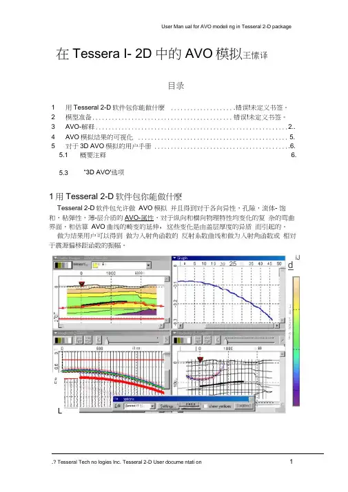
3AVO-解释 ........................................................... 2.. 4AVO 模拟结果的可视化 .............................................. 5. 5 对于3D AVO 模拟的用户手册 .. (6)1用Tesseral 2-D 软件包你能做什麽Tesseral 2-D 软件包允许做 AVO 模拟 并且得到对于各向异性,孔隙,流体- 饱和,粘弹性,薄-层介质的AVO-属性,对于纵向和横向物理特性均变化的复 杂的弯曲界面,和估算 AVO 曲线的畸变的延伸,这些变化是由盖层厚度的异质 而引起的。
做为结果用户可以得到 做为入射角函数的 反射系数曲线和做为入射角函数或 相对于震源偏移距函数的振幅。
5.1 概要注释6.5.3“3D AVO'选项iJ d o □2000 LJ」 10 co20 Oi : 寸 □:二. □I- soJlcxted IT 巴 20 25 I | 匚bieblg! [ l bdpgohi r 甲 5 GaHlPl MBNadDl: ConppoL J ^□nlriwc! g u口昌 tJDSE Sam2模型准备2.1在模型建立器中当前模型选择一个多边形做为AVO模拟的分界线。
从Run"的下拉菜单上选择“AVO Modeling”:Prepare Model Prcicessing CLUSTER: Create Task...I” |Vertical Incidence Modeling 迄Scalar Modeling 淳.ARiistic Mod el rig 祿Elastic Modeling 於ElasticAnisotropic ModelingAVO Modelling2.2 在产生的AVO Computati on Parameters 对话框中:指定检波器从AVO模拟目标边界垂直的位移。
Tesseral 2-D 全波场模拟用户手册
王愫译目录1总体说明 (5)1.1 关于文档 5 1.2 你能用Tesseral 2-D 软件包做什麽 5 1.3 浏览器7 1.4 数据输入/输出8 1.5 启动8 2用模型建立创建一个模型 (9)2.1 当你第一次开始应用Tesseral 2-D 9 2.2 模型建立器面板9 2.3 模型建立器菜单和工具条10 2.4 "Framework"“构架”会话11 2.5 "Cross-section"“剖面”页11 2.6 "Source"“震源”页13 2.7 "Observation"“观测系统”页16 2.8 "Reflector"“反射层”页18 2.9 "Signal"“信号”页18 2.10 “Polygon”“多边形”会话212.10.1 “Physical Properties”“物理特征值”页22 2.11 “Options”“选项”会话252.11.1 “General”“概要”页262.11.2 “Measure units”“量度单位”页262.11.3 "Graphics"“图形”页27 2.12 模型建立器的技巧272.12.1 目标移动272.12.2 “Source”“震源”和“Receiver”“接收器”目标282.12.3画多边形282.12.4 梯度/复参数分配292.12.5 随后的模型修改302.12.6 画多边形总结302.12.7 修改多边形31 2.13 观察一个多边形31 2.14 图片放大33 2.15 “Define Scale”定义比例尺会话33 2.16 等容和调整比例尺35 2.17 图片拖拽35 2.18 保存模型数据35 2.19 打开模型数据36 2.20 模型硬拷贝37 2.21 颜色比例柱状图38 2.22 颜色选项382.23 坐标符号39 2.24 “Tune position”“调整位置”会话选项40 2.25 震源方式41 2.26 从模型建立器运行计算引擎43 2.27 应用主窗口的管理面板44 2.28 改变主窗口的尺寸45 2.29 图片叠合45 3全-波模拟计算 (47)3.1 “Computation”“计算”会话47 3.2 “Report”“报告”窗48 3.3 波场计算48 3.4 波动方程计算方式49 4数据管理协议 (50)5用浏览器分析结果 (51)5.1 浏览器窗51 5.2 以其它标准格式表示的文件51 5.3 浏览器窗口菜单和工具条51 5.4 “File”“文件”菜单弹出列表51 5.5 “View”“浏览”菜单弹出列表51 5.6 图片可视化选项525.6.4 附加的单-道转换功能55 5.7 浏览波场快照56 5.8 用浏览器面板中的图片处理56 5.9 从浏览器硬拷贝56 5.10 在主软件包的窗口做图片和电影56 5.11 浏览器的“Run”“运行”菜单条目57 5.12 复杂的数据转换57 6发现并修理故障 (59)附录 1. 模型建立器的(.tam)模型转换为网格模型 (61)附录 2. 多分区网格 (61)附录 3. 井-曲线数据 ( LAS格式) 转换 (61)附录 4. 以网格格式表现介质模型的转换 (62)附录5. 以text格式表示模型的输入-输出 (63)附录 6. 以SEGY格式表示数据的转换 (63)6.1 模型63 6.2 道集64 6.3 sgy-模型转换到 tgr-模型64 6.4 在Tesseral-2D 软件包中用SEGY-道集67 6.5 从多个SEGY 文件得到各向异性参数的介质模型686.5.1 为加载准备各向异性参数的SEGY文件686.5.2 建立一个包含各向异性参数的tgr-模型文件69附录 7. 在Tesseral 2-D中的АVО模拟 (70)1总体说明1.1关于文档Tesseral 2-D软件包的文档由一定的文件数量组成(看..\_ Index of Tesseral 2-D User Documents _.pdf). 在所给的文档中给出了该软件包核心功能的描述。
Tesseral Pro手册(中文版)
Tesseral 中文 用户手册(全)
在PC机上地震和声波场建模程序Tesseral 2-D 全波建模程序用户手册目录1. 概述 (4)1.1 建模器 (4)1.2 计算引擎 (4)1.3 浏览器 (5)1.7 数据输入/输出 (5)2. 启动 (5)3. 用建模器创建模型 (6)3.1 第一次启动 (6)3.2 建模器面版 (6)3.3 建模器菜单和工具条 (7)3.4 剖面页 (7)3.6 观测系统页 (12)3.7 多边形 (15)3.8 静态物理参数 (18)3.9 通用菜单条目 (18)3.10 选项对话框 (19)3.11 炮点和接收点对象 (21)3.12 画模型 (22)3.13 梯度/复合参数分布 (23)3.14 模型修改 (24)3.15 修改多边形 (25)3.16 观看模型 (26)3.17 图片放大 (28)3.18 等轴和调整比例尺 (30)3.19 拖动图片 (30)3.20 保存模型数据 (30)3.21 模型硬拷贝 (33)3.22 彩色色标 (34)3.23 颜色选项 (34)3.24 坐标标记 (35)3.25 “微调位置” 对话框选项 (37)3.26 震源模式 (37)3.27 在建模器中运行计算引擎 (39)3.28 应用主窗口的管理 (40)3.29 改变主窗口的大小 (41)3.30 图片重叠 (42)3.31 下一版本的窗格特征 (43)4. 全波场模型计算 (45)4.1 计算对话框 (45)4.2 报告窗口. (46)4.3 波场成分 (47)5. 数据管理约定 (48)6. 用浏览器分析成果 (50)6.1 浏览器面板 (50)6.2 别的标准格式文件 (50)6.3 浏览器窗口菜单和工具条 (50)6.4 “File” 下拉菜单列表 (51)6.5 “View” 下拉菜单列表: (52)6.6 图片视觉选项 (53)6.7 浏览快照 (57)6.8 在浏览器中对图片处理 (57)6.9 硬拷贝 (57)6.10 浏览器“Run” 菜单条目 (57)6.11 [++下一版] 累加 (57)6.12 网格转换 (58)7. 问题解答 (59)8. 附录A 转换模型到网格格式 (61)9. 附录B 多分区网格 (61)10. 附录C 测井曲线文件(.las)输入 (62)11. 附录D 网格模型计算 (64)12. 附录E 模型文本文件的输入/输出 (65)1.概述Tesseral 2-D 全波波场建模软件包版本2.5包含3个主要的部分: Modelbuilder(建模器),Computational Engine(计算引擎)和 Viewer(浏览器)。
机器人史宾v2说明书
机器人史宾v2说明书导言祝贺选择罗伯萨皮尔?2版,新一代罗伯萨皮尔?具有新的技术和个性。
并且有了更先进的运动能力和互动式传感器,新功能程序,语言能力,和独特的个性。
具有思想,感情和多种能力结合的机器人时代已经来到~请务必精心阅读本手册全面理解您的新的和改进的机器人的许多特点。
此包包含:1个罗伯萨皮尔?2版1个控制器1个绿色保龄球球3 个红保龄球瓶快速入门指南马上见识一些罗伯萨皮尔?V2的非常酷的功能,插入他的电池(见5- 6)打开它(见第13页),并按照下列指示:停止:按停止罗伯萨皮尔?2版将停止目前的行动。
演示1:按下去将执行预置的舞蹈。
演示2:SHIFT1+D按顺序执行罗伯萨皮尔?V2的一系列动作的演示静躺/坐起来/静躺/站起来:SHIFT2+D罗伯萨皮尔?V2版将循环执行这些功能。
左摇杆L=步行:步行是受左摇杆控制;主要有前进,后退,左,右,和对角线运动。
右摇杆R=头和上身:控制权可以控制上身基本运动。
胳膊:SHIFT1+SHIFT2+D右摇杆和SHIFT1、SHIFT2按钮配合使用,可以控制罗伯萨皮尔?V2的胳膊。
自由漫步:让罗伯萨皮尔?2版自由漫步,自主探索他的环境。
不过确定他在地板上面再开始。
~红外视觉:与罗伯萨皮尔?2版直接交流。
把你的手在他面前,他会跟踪你的动作。
02内容表格•电池信息:第5- 6 •罗伯萨皮尔?2版简介:第7页•控制器概述:第8页•控制器综述功能图:左侧第9-10页,右侧第11- 12页•基本操作:电源开关第13页访问控制命令第13页停止第14页散步第14页头部和上身第15页胳膊第16页•演示和动画:舞蹈演示第17页运动演示第17页右臂命令第17页左臂命令第17页躺下/坐起来/静躺/站起来第17页起床第17页行动第17- 18页•重置:全复位第19页快速复位/步态变化第25页睡眠/唤醒第25页关闭电源第19页声波传感器开/关19页视觉系统开/关19页•自由漫游: 自由漫游第20页待机模式第20也03目录•视觉系统:视觉系统开/关21页远距离红外视觉21页近距离红外视觉21页退缩反应28页躲开物体28页•彩色摄像:颜色识别第23 – 25页彩色摄像头设置25页闪烁26页•声波传感器:声波传感器开/关26页听力第26 - 27倾斜传感器27页握传感器/举高第27 - 28手套传感器第29页脚传感器第29页•编程:编程键30页定位程序目录30页主定位程序模式第30 – 32页左,右定位程序模式第32页控制器程序目录第32页主要程序目录第32 – 33页退出程序第33页子程序第33 - 34声音和视觉程序模式p.34 •警戒模式:35页•机器人互动:罗伯萨皮尔?2版第36页罗伯萨皮尔恐龙第37页罗伯萨皮尔狗第37页重要提示第38页04电池信息电池要求:罗伯萨皮尔?2版的身体和大脑罗伯萨皮尔?2版是由6 ×1号电池(不包括在设备内)和4 ×7号电池(不包括)。
Tesseral 2-D Tutoriall (Eng)
Tesseral 2-D Tutorial(1) Making a NEW modelTo initiate the Tesseral system, click on the Tesseral iconThe blank Tesseral screen appears. Only one of six possible empty panes appears. We want to build a new model, define a VSP survey parameters and run the forward modeling.If you double click mb1 in the titlepart of the pane (blue colored area),then the six panels will appear.Double clicking mb1 in the 1st panereturns to window to a single paneview.To build the model itself, we have to:Define the model boundariesBuild polygon layers inside the model boundariesDefine the physical parameters of the layersEngage the proper modeling algorithm for our purposes Special care must be taken to input the model layers so that layer merging and truncation are handled properly.To open up a new model, go toFileNewA default model appears. The menu is the Framework menu and will be used to define the model boundaries (cross-section), and Source(s) and receiver(s) configuration.Let’s define the model boundaries to be –150 on the top, 3000 m down to the bottom, -1000 m to the left of our “0”, and 1400 m to the East.We can make the surface invisible. This means that upgoing waves will not reflect back down into the model. The Framework/Cross-section menushould look like(2) Making the first model polygonWhen we fill this in, and then click on OK, we can define our 1st polygonIn the menu, we can start by defining the P-wave velocity. The S-wave velocity and density will assume default values (the defaults will be used when the boxes under “Default” are ticked).One of the options that we have is to define the layer physical properties using the sample parameter table. The table has been set up for various rock types with their minimum, average and maximum P- and S-wave velocities and Densities. We pull down the sample list and select, in this case, “Sediments” …Choose the Anhydrite [min]sampleWe can apply a pattern tothe layer by clicking on“Apply Pattern”. Thepattern for the sedimentsappears in the pattern box.Next, let’stransfer our “sample list” parameters to the “Velocities” and “Density” entrie s. The altered Polygon definition menu now looks like …When we click OK, the polygon layer appearsWe want to show how to move the source and receiver line to a new elevation. To move the source, we place the cursor over the source (shown as a re d triangle … delta) and pull the source to our new location. To perform the same task for the receivers, we place the cursor on top of a receiver, click mb1 and pull the entire line up receivers up to the source location.(3) Making the second polygon (simple flat layer)Place the cursor in the New Polygon icon (shown below) and click mb1. The cursor turns into a polygon shape with a plus sign below it.Locate the cursor outside of the left boundary at about the 500 m mark (see the Z value at the bottom of the Tesseral window).Click once and extend the line horizontally over to a position just outside of the right boundary. Double clicking mb1 will close the polygon down to the bottom of the model. This is shown below.After the double-click, the Polygon property menu appears(fill in 1700 m/s for the P-wave velocity)Notice the boundaries of the second polygon. After filling in the Velocities(defaulting the S-wave velocity and density), press OK to complete the model entry.(4) Designing the third and fourth polygonPolygon 3 will start from the left side of the model and truncate against Polygon 4. How do we do this? We first input Polygon 3. Then we construct Polygon 4 so that it cuts through Polygon 3. Let’s put in polygon 3.Place the cursor inside Polygon 2 (where the new polygon will be created) and click mb3. Choose the “New polygon” menu item …Place the cursor at 1222 m on the outside of the left boundary, click mb1, bring the cursor directly across the model (also at 1222 m depth) to the outside of the right boundary, double click mb1 to complete the polygon and bring up the Properties menu … fill in the P wave velocity of 2000 m/s.Click Ok to see the new layer 3. Inside of the 3rd layer, click mb3 and select New Polygon … Let’s start drawing the new polygonThe polygon is drawn over to the right boundary (just outside of it) double click mb1 to close the polygon. Define the velocities and densities. Name the polygon “Polygon 4” as shown belowClick Ok to see model. The third layer is truncated against layer 4. This is similar to the shales abutting against the carbonate reefs.(5) Final layer cutting across two previously defined layersIn this layer input, the layer penetrates both polygons 3 and 4. Initiate the New Polygon cursor by clicking mb3 inside la yer 4 … and clicking the New Polygon icon …Drawthepolygon starting just outside the left boundary at ~ 1800 m, draw the line through layers 3 and 4 as shown, draw the line to just below the model boundary and then extend the line back to the outside of the left model boundary (see below)When you place the cursor to the left of the left boundary and double click, the polygon closes (see blue ellipse) and the Polygon menu box appearsFor polygon 5, fill in the velocity values as shown below (and then click OK)Click OK and polygon 5 is done.( 6 ) Double checking the units of measurementPlace the cursor over the hammer as shown below and bring up the Properties menuClick ont he “Measure Units” tab to reveal the measurement system used in the modeling.Let’s look at how to change the units. Click on the “down” arrow located on the right hand side of the “Time” box. It reveals that we can choose to enter time units in s (seconds) or ms (milliseconds).( 7 ) Using FRAMEWORK to set the sources (on the surface) and receivers (in the borehole)Choose the FRAMEWORK iconas shown on the rightThe basic Framework window appears …Click on the Source tab to define the source configurationTo set the receiver locations, click the Observation Tab. The default menu isSet the downhole receivers to start at -150 m to 3000 m depth at a sonde depth interval of 30 m. Start the recording at 0 ms and stop at 1500 ms. The sample rate for the recording is 2 ms. Note that the number of depth levels, time samples, sources and pictures are shown on top of the menu boxes.The setup for the sources and receivers now looks likeLet us label the shots and receivers using the“Show receiver Numbers”The shots and receivers now appearwith numerical labels …We now want to fine tune the positions of the sources using the fine tune icon …The procedure is to locate the cursor at the location of the object that you want to move, a faint cursor image lies on top of the object, type in the new coordinates for the object and then click enter. In this example, we want to move the entire row of sources. Moving the cursor to the first source locates the first source at x= -400 and z= -150 m, as shown below. With the source highlighted by the cursor, type in 200 for X and –150 for Z (to shift into Z window us e “Tab” keyboard button) in the Tune menu …Press “Enter” in the Tune Position menu to move the sources to the right.The leftmost source now has coordinates of X=200 m and Z=-150 m. Close the fine tune box by clicking on the X in the upper right hand corner.( 8 ) Inputting a deviated boreholeWe start by creating a new polygon using theiconDraw in the deviated well (use the X and Zvalues shown at the bottom bar). Thegreen circles show the chosen “break inslope” points in the de viated well. Ourtask is to create an artificial polygon andthen project the polygon onto the deviatedwell.Double click mb1 at the bottom of thedeviated well to bring up the polygondefinition box.Click the OK box becausethis is a dummy polygonand the parameters do notneed to be specified.Upon clicking OK with mb1, thepolygon is completed, as shown below.Now we want to collapse the polygononto the deviated well trace.To do this, we use a utility under “Edit”to project the receivers onto the traceof the borehole.This is shown below …Edit > Project > ReceiversWe can now collapse the polygon into a single line. Place the cursor inside the polygon that you just made using the deviated borehole. Click mb3 to bring the menu shown below …Choose Cut PolygonNext what should appear isthe trace of the deviatedborehole with receiver levelssuperimposed onto thetrace …We are now ready to run the Finite Difference modeling software.( 9 ) creating the modeled data using the F-D elastic softwareA good practice is to save the model that you just created. To do this, click on File > Save asThe Save As window appears …Create a new folder (1). Rename the folder by placing the cursor inside the name box of the folder (2), click mb1, edit in a new name and click mb1 outside of the name box (3).Double click mb1 on the folder icon (named Tutorial). This puts you into the model name leve l. Edit the “File Name” to be Model 1 (1), click mb1 on the Save button (2). This puts the model name into the Tesseral database (3).Now that the model has been saved, we can initiate the modeling software. The options areVertical Incidence ModelingScalar ModelingAcoustic ModelingElastic modelingElastic Anisotropic ModelingTo initiate the menu, go to “Run” on the Tesseral main menu …The first step in the F-D routine is to build the model grid. The grid spacing is determined by the dominant frequency of the source wavelet. The grid spacing is chosen to avoid grid aliasing.Once the grid is built, the computation begins for source number 1. Note the propagation of the wavefront and the VSP downgoing event. The downgoing wavefront is detected at the geophone locations in the borehole.Asthe computation continues, we see that the downgoing wavefield is about to reflect from the “reef-like” structure.Note the reflected upgoing wavefront. The amplitude of the downgoing event can be 100 times larger than the upgoing events … so the upgoing VSP event is difficult to see on the VSP (on the left) without proper scaling.To equalize the up- and downgoing VSP events and wavefronts for display purposes, we use the visualization options … use the icon shown belowIncrease the equalize percentage to view the VSP and wavefront dataPress Apply to allThe computation continues from the first source to the third source …Following the computation, the screen shows the model, last computed VSP data and the model with animation options.Place the cursor between the top and bottoms panel until it change shape (two horizontal lines). This allows one to expand the bottom panels to fill almost the entire working area by dragging up the panel boundaries. Position the bottom panel so they lookWe see a time step line on the VSP data. This is used during the animation process. The animation process will replay the generation of the wavefronts in a movie fashion. The time step line shows how the VSP data is being generated as the wavefronts in the movie propagate. The animation icons in the two panels look likeTo animate the wavefront propagation, click mb1 on the animation button (shown circled above). Some example displays areEqualize the display using theVisualization options(10) Merging all the shots into one file for wavefront/event analysisOn the previous page, we saw that one record could be replayed back using event and wavefront animation. When we have many sources as in a multi-offset VSP survey, we would want to control what source we are viewing. To do this, we merge the “gather” files together … meaning that all 3 VSP datasets and wavefront movies can be merged into two large files, one for the VSP data and the other for the wavefield propagation. To do this we begin at the end of the computation step that shows the 3rd VSP dataset (GathEP-3.tgr) and the 3rd sources’ wavefront record (SnapEP-3.tgr). We will now collect the 3 datasets into merged datafiles … T he starting point is shown belowWe now want to enlarge the two lower panes to fill up the entry working space. To do this, we place the cursor at the top edge of one of the two lower panes. We see that the cursor changes to the shape …Pull up the panel border … to create the picture shown below …Next, change the visualization options to gain thedata … use the icon and fill in the menu as belowHighlight the left bottom panel (for the VSP data). The data from the 3rd source is shown in this panel. We can start the merge process my going to RUN > Grid Merge …The computational tracker menu appears …Once this process is complete, then you are given the choice to delete or retain the 3 individual VSP data files that have been merged into Model 1 + GathEP.tgr.So, the files GathEP-1.tgr, GathEP-2.tgr, GathEP-3.tgr GathEP.tgrWe can now do the same with the wavefront snapshots … highlight the Snapshot title bar … a nd Run > Grid MergeThe computational menu appears and the option to delete the individual input files gives us the option to save disk space by deleting the input files…We now have the Gath-EP.tgr and Snap-EP.tgr merged files to help us examine all of the source datasets easily …We can look at the three shots, one at a time, by using the sliding bar on the Gath-EP.tgr panel … as shown belowSOURCE 1 …SOURCE 2SOURCE 3APPENDIX AInputting log curves in LAS format fand model buildingTo load LAS files into Tesseral, we need to have a default model already defined. We then input a log and ask the program to generate a model from the log (using P- and SV-velocities derived from the input sonic logs and the density taken from the input density log).T o generate the default model, let us start at the beginning …initiate the Tesseral system using the Tesseral iconThe main Tesseral menu appears … Click mb1 on the Framework icon (circl ed in red), … , click on the Observations tab, change the bottom and right boundary distances and click OK.Fill in the Polygonproperties menu as shownand press OK. This willcreate a “dummy” model toplace the well logs into.NOTE: the depth of themodel should be deeperthan the deepest log depthThe single polygon model appear …To bring in the LAS file, use File > Open > as shown below …Search for LAS files using “Files of type” …Choose the Wid s file…The next menu allows you to select which curves from the well you want to put into the model … Choose “Add All” …A rectangle appears inside the model which can be positioned where you want t o place it by dragging the box with the cursor …once the rectangle is inposition, click mb1 to bring inthe logs …Click mb3 inside the wellrectangle to bring up the menuthat has the Properties option ..In this menu, we can change the LineProperty of the chosen Log … This willassist us in telling one curve from theother …Select the Shear sonic curve and click onLine PropertyChoose the green color …Press Ok to see the curve changecolor in the model display …Next, we want to generate the model using thewell log curves as input … the model willobviously be composed of horizontal layers …Choose the curve names that match the model property and choose 6 (versus 10 for the deviation clearence) as the curves do not show drastic jumps in their overall range of values …Here we see the model … some of the layers are thick and some are thin. The thin layers are nearer to the bottom of the borehole ..Each layer’s polygon can be seen by clicking mb1 within the layerTo zoom in on one of the thin layers near the bottom of the borehole, we use the magnifying tool … Once the magnifying tool is active, click mb1 to start one side of the zoom box, drag to enlarge the box and then click mb1 to close the box …To exit from magnification mode click mb2 or chose (pointing) from toolbar. To choose a layer, click mb1 on the layer. To bring up the Polygon properties menu, double click mb1 on the s elected layer … you can now change the layer properties …Let’s save the model we have created … to do thisClick on File > Save As >Within the Save As menu, type in the model name and Save。
最新Tesseral+2D正演模拟培训讲义
FOLLOW ME (正演模拟培训讲义)从一个bmp 文件建立一个模型并进行全波场模拟:(一)粘贴一个bmp 文件1、给一个深度比例尺的速度—深度模型图在画图软件中把模型的比例尺和范围做准,并输出一个bmp 格式文件备用。
2、在工具条上点击 打开Tesseral 主界面(图1),并填写正确的顶、底、左、右坐标,并在Surface 组参数中选“Invisible ”不可见地表 ,如果是地震(声波)波场模拟,地表一定不能出现。
“Invisible ”表示上行波将不再向下反射回到该模型按“确定”后,在删掉跳出的物理参数填写表后,出现一个空白的坐标网格图(图2)。
图1 图23、在工具条上选择 点左键光标变为多边形,表示可以开始画图。
手工在屏幕上画多边形请看”Tutorial-Hinds&Kuzmiski May 2002”。
现在讲如何从一个bmp 文件描绘一个模型。
从坐标外的一点开始,画一个矩形后双击,出现一个红色边界的矩形框后出现参数表,可以不填,点击“确定”,则完成了一个空白的矩形的建立(图3)。
4.点击打开文件,再点击Picture Files ,选出准备好的bmp 文件(图4)。
图3 图45.文件显示的窗口中,确认所选的顶、底、左、右坐标无误后,点击OK(图5)。
6.bmp文件就以正确的比例贴在Tesseral 的绘多边形的窗口上(图6)。
图5图6(二)描绘多边形1.开始描绘第一个多边形,从左侧的坐标线外起始,然后精细地用鼠标描绘地形线到坐标的右侧外点一下,然后下拉到底部,点一下,再向左下角拉线,点一下,然后双击左键矩形封闭。
在出现的参数表上填写第一层的参数2800米,其余用缺省值(图7)。
2.完成后点击OK,第一个多边形则做好了(图8)。
图7图83.为了看清楚原图的线,也可以选用 消色键(图9)。
4.画以下的多边形,原则是整的多边形从坐标线外起始画,内部多边形在某一个多边形内部封闭,当两个多边形重叠以最上面呈现的部分有效,压在下面的失效(每个多边形的参数表,你都填写正确的P 波参数,其余用缺省值,原则是从上到下,从整到零。
TES数位式照度计操作规程
TES数位式照度计操作规程
1.操作规程
1.1打开电源。
1.2选择适合测量档位。
1.3打开光检测器头盖,并将光检测器放在欲测光源之水平位置。
1.4读取照度计LCD之测量值。
1.5读取之测量值,如左侧最高位数“1”显示,即表示过载现象,应立刻选择较高档位测量。
注;设定20,000Lux /fc档位时,所显不读值须×10倍才是测量的真值。
设定200,000Lux档位时,所显示读值须×100倍。
1.6读值锁定开关:按HOLD开关一下LCD显示“H”符号,且显示锁定读值。
再按一下则可取消读值锁定功能。
1.7峰值锁定;欲测量光脉冲信号,按PEAK开关—次,LCD显示"P"符号,即脉冲蜂值,再按PEAK开关一次,即回复正常测试。
1.8测量工作完成后,将光检测器头盖盖回,电源开关切至OFF。
2期间核查
3维护保养
按该仪器使用说明书有关要求,进行日常的维护保养,并对该仪器的使用状况和维护保养情况每年作一次记录备案待查。
3.1请勿在高温、高湿场所下测量。
3.2使用时,光检测器需保持干净,光源测试参考准位在受光球而正顶端。
3.3电池电力不足时,LCD上出现“BT”指示,表示须更换电池。
Tesseral 2-D 全波场模拟用户手册.
用户手册在个人计算机上的声波和地震波模拟Tesseral 2-D 全波场模拟用户手册目录1. 概述 (4)1.1 模型建立器 (4)1.2 计算引擎 (4)1.3 浏览器 (5)1.7 数据输入/输出 (5)2. 开始 (6)3. 用模型建立器创建一个模型 (6)3.1 当你首次应用Tesseral 2-D (6)3.2 模型建立器框 (6)3.3模型建立器菜单和工具栏 (7)3.4 "Cross-section" 页 (7)3.5 "Source" 页 (9)3.6 "Observation" 页 (12)3.7 “Polygon” 会话 (14)3.8 静态物理参数 (17)3.9 共同的菜单条目 (17)3.10 “Options” 会话 (18)3.11 “Source”和“Receiver” 对象 (20)3.12 画模型 (20)3.13 梯度/复杂参数的分配 (21)3.14 稍后模型的修改 (22)3.15 修改多边型Polygon (23)3.16 浏览模型 (24)3.17图画放大 (25)3.18 等大的和调整比例 (27)3.19 图画拖动 (27)3.20 保存模型资料 (27)3.21 模型硬拷贝 (29)3.22 彩色比例色棒 (30)3.23 彩色选项 (30)3.24 坐标符号 (31)3.25 “Tune position” 会话选项 (33)3.26 Source方式 (33)3.27从模型建立器运行计算引擎 (35)3.28应用主窗口的管理框 (36)3.29 主窗口尺寸的改变 (37)3.30 图画叠合 (37)3.31 计划下一个版本的特征 (39)4. 全波模拟计算 (40)4.1 “Computation” 会话 (40)4.2 “Report” 窗. (41)4.3 波场计算 (42)4.4 方程式计算方式 (42)5. 数据管理协定 (43)6. 用浏览器分析结果 (44)6.1 浏览框 (44)6.2 其他标准格式的文件 (44)6.3 浏览窗菜单和工具栏 (44)6.4 “File” 菜单 Popup列表 (45)6.5 “View” 菜单 Popup 列表: (46)6.6 图画可示化选项. (47)6.7 浏览波场快照 (50)6.8 在浏览器中有关图画的管理 (50)6.9 硬拷贝 (50)6.10 浏览器“Run” 菜单项目 (50)6.11 [++ 下一个版本] 总和 (50)6.12 网格转换 (51)7. 发现并修理故障 (52)8. 附录 A. 转换模型到网格形式 (53)9. 附录B. 多分割网格 (54)10. 附录C. 井曲线文件 ( .LAS) 输入 (54)11. 附录 D. 用网格文件计算 (56)12. 附录 E. 从text文件输出和输入模型 (57)1.概述Tesseral 2-D全波场模拟软件包含四个主要部分: 模型建立器, 计算引擎, 浏览器和处理。
- 1、下载文档前请自行甄别文档内容的完整性,平台不提供额外的编辑、内容补充、找答案等附加服务。
- 2、"仅部分预览"的文档,不可在线预览部分如存在完整性等问题,可反馈申请退款(可完整预览的文档不适用该条件!)。
- 3、如文档侵犯您的权益,请联系客服反馈,我们会尽快为您处理(人工客服工作时间:9:00-18:30)。
在PC机上地震和声波场建模程序Tesseral 2-D 全波建模程序用户手册目录1. 概述 (4)1.1 建模器 (4)1.2 计算引擎 (4)1.3 浏览器 (5)1.7 数据输入/输出 (5)2. 启动 (5)3. 用建模器创建模型 (6)3.1 第一次启动 (6)3.2 建模器面版 (6)3.3 建模器菜单和工具条 (7)3.4 剖面页 (7)3.6 观测系统页 (12)3.7 多边形 (15)3.8 静态物理参数 (18)3.9 通用菜单条目 (18)3.10 选项对话框 (19)3.11 炮点和接收点对象 (21)3.12 画模型 (22)3.13 梯度/复合参数分布 (23)3.14 模型修改 (24)3.15 修改多边形 (25)3.16 观看模型 (26)3.17 图片放大 (28)3.18 等轴和调整比例尺 (30)3.19 拖动图片 (30)3.20 保存模型数据 (30)3.21 模型硬拷贝 (33)3.22 彩色色标 (34)3.23 颜色选项 (34)3.24 坐标标记 (35)3.25 “微调位置” 对话框选项 (37)3.26 震源模式 (37)3.27 在建模器中运行计算引擎 (39)3.28 应用主窗口的管理 (40)3.29 改变主窗口的大小 (41)3.30 图片重叠 (42)3.31 下一版本的窗格特征 (43)4. 全波场模型计算 (45)4.1 计算对话框 (45)4.2 报告窗口. (46)4.3 波场成分 (47)5. 数据管理约定 (48)6. 用浏览器分析成果 (50)6.1 浏览器面板 (50)6.2 别的标准格式文件 (50)6.3 浏览器窗口菜单和工具条 (50)6.4 “File” 下拉菜单列表 (51)6.5 “View” 下拉菜单列表: (52)6.6 图片视觉选项 (53)6.7 浏览快照 (57)6.8 在浏览器中对图片处理 (57)6.9 硬拷贝 (57)6.10 浏览器“Run” 菜单条目 (57)6.11 [++下一版] 累加 (57)6.12 网格转换 (58)7. 问题解答 (59)8. 附录A 转换模型到网格格式 (61)9. 附录B 多分区网格 (61)10. 附录C 测井曲线文件(.las)输入 (62)11. 附录D 网格模型计算 (64)12. 附录E 模型文本文件的输入/输出 (65)1.概述Tesseral 2-D 全波波场建模软件包版本 2.5包含3个主要的部分: Modelbuilder(建模器),Computational Engine(计算引擎)和Viewer(浏览器)。
1.1建模器允许用户构建一个二维的密度-速度地质剖面模型,然后运行计算引擎中的一个模型程序。
1.2计算引擎计算合成地震记录和拍摄系列快照,目前支持5种波动方程的计算:1.2.1 垂直入射模型提供一种相对较快的估计反射波时间和振幅的方法,该方法假设地震能量传播是严格垂直的一维传播,在该假设情况下,不考虑地震能量的耗散。
.1.2.2 标量波动方程模型是非均匀介质中波场效应最简单的近似,它只考虑压缩波的传播,不理睬密度变化。
这个方法对于估计波的运动是很有用的,它的计算速度能比声波方程模型快30%。
1.2.3 声波方程模型使用户能估算实际地质情况中地震能量传播的二维波场效应,它忽略固体介质中的刚度,即是说,这是一种理想的流体介质,在该介质中横波的速度为零。
这种近似对于固体的计算仍然有用,当大部分地震能量传播到不连续介质时,转换波的振幅是很小的,可以忽略不计。
声波方程模型计算比垂直入射模型慢,但比弹性波方程模型要快。
声波方程模型和垂直入射模型仅考虑纵波速度和密度特性。
1.2.4 弹性波动方程模型是这个软件包中最综合的工具,产生的结果最接近固体介质的实际条件,包含了转换波和横波效应。
它不仅考虑密度和纵波的分布也要求知道对应横波的速度,它的计算时间是声波方程的两倍。
横波速度在模型的某些区域可以为零,这样就在模型中形成固体和液体两种介质。
1.1.1 各向异性弹性波动方程模型是弹性波动方程的一个变异,模型在纵向和横向的物理特征的变化被考虑。
这个公式允许粗略地模拟各向异性介质的响应(§ 3.7.3.4). 它花费的时间是弹性波动方程模型(各向同性)的三倍。
1.2.6 计算时间不仅依赖于方程的类型,同样也依赖于模型的尺寸的大小(成正比)。
纵波最小速度的降低和最大速度的提高会加大计算的时间。
震源的主频也是很关键的参数,因为计算时间与主频三次方成正比。
正常情况下,中小模型(从1*1 km模型、震源主频100HZ以内到10*10km模型、震源主频小于30HZ)的计算时间(PC 500MHz)从一分钟到几小时不等。
1.3浏览器被用于观看两种计算结果:炮集和快照。
计算的炮集是一个合成记录,类似于野外观测接收排列得到的数据集,计算结果将和实际数据进行比较。
通过观看和分析模型计算波场传播的成功快照,将帮助用户识别地震同相轴。
1.4 数据通常被存储在与特定剖面相对应的目录中(§ 5).1.5 由建模器形成的数据是模型数据,是一个带有扩展名“.tam”的文本文件。
1.6 由计算引擎产生的网格文件,扩展名是“.tgr”,为二进制文件。
1.7数据输入/输出标准格式或一些别的软件包数据格式能够输入到建模器中。
同样,数据也能够从建模器或浏览器中输出(§12.8) 。
成果能够以几种格式输出,以便在别的软件包中作进一步的分析和处理,或者被转换为不同的光栅文件格式(§6.4.3)。
2.启动2.1 模型源数据与建模器相对应,成果与浏览器相对应。
点击这些带图标的文件将调用这些文件的Tesseral 2-D应用程序。
2.2 你可以从"Start"→"Programs"→"Tesseral.exe" 启动Tesseral 2-D程序,也可以点击快捷图标启动。
2.3 用户可用拖放(“drag and drop”)数据文件来打开对应的Tesseral 2-D 应用程序。
3.用建模器创建模型3.1第一次启动Tesseral 2-D应用程序,建模器面板自动地打开,对于第一次阅读和初次建模,你可以跳过软件包选项和对话框描述的细节,当你需要时再返回来阅读它。
有几种办法可以重排应用程序主窗口(§ 3.28)。
3.2建模器面版允许你在屏幕上构建图形化的模型、输入速度和密度的分布、设计观测系统参数,并运行计算模块。
3.2.1 下图是一个简单但相当弯曲的模型剖面,它象由一组多边形叠合而成。
3.2.2 多边形根据用户画图的先后次序排列起来,后面画的多边形(部分或全部)覆盖在前面画之上。
建立模型最常用的顺序是从模型的顶部到底部顺序画出。
以后可以插入和删除多边形。
3.2.3 多边形允许在选择的区域内局部地分布物理参数。
通常用户看到的是没有被覆盖的多边形部分。
这些可见部分是有效面积,即要被计算的部分,连同其他可见部分,构成实际要表述的模型。
3.3建模器菜单和工具条首先让我们看看菜单(上行文字)和工具条(下行图标):3.3.1为了建立新的模型,你应该执行“File” “New”菜单顺序,或按下工具条上按钮。
3.3.2 当建立新模型时,"Framework" 对话框出现,该对话框包含四页:a ) "Cross-section",b ) "Source",c ) "Observation"d ) “Horizons”。
这个对话框可以在任何时候由按下按钮或者在“Edit”下拉菜单中选中对应条目调用。
3.4剖面页允许定义模型的方框、名字和设置计算方法。
3.4.1 模型名:如果有必要的话,模型剖面除了有一一对应的模型文件外,可以额外添加一个名字。
3.4.2 模型方框:规定了模型的面积,修改"Left", "Top", "Right", 和"Bottom"的值,就改变了模型面积。
3.4.3 “Computation”组包含一些设置计算引擎的参数。
3.4.3.1 地表组按钮:3.4.3.1.1 不可见(“Invisible” 选中)地表,如果是地震(声波)波场模型,地表一定不能出现。
3.4.3.1.2“Free” 产生一个“真正”的自由界面,在自由界面上波根据界面条件被反射,反射波相位与入射波相位相反。
3.4.3.1.3 对于“Static” 选项,来自界面的反射波将和入射波有同样的相位(速度/密度由低到高),如果震源被放在靠近界面的地方,震源的最初脉冲将被来自模型界面的正反射系数修改。
“Static” 选项在标量方程中不起作用(§ 1.2.2)。
3.4.3.2 网格单元的最小参数值:3.4.3.2.1 最小纵波速度(“Velocity”)。
最小速度越高,网格单元尺寸越大,缺省值(选中对应框)为模型输入的实际最小值。
输入更高的值(可到实际值的200%),用户可以控制计算的速度和质量。
3.4.3.2.2 最小波长(“Wavelength”),最小波长越小,网格尺寸越小,缺省值(选中对应的框)为模型输入的实际最小波长值。
输入一个更小的值(可小于实际值的25%),能增加网格的精度(波场模型),在小不均质(但规则)模型或者为了避免横波耗散,常常使用更小的波长。
3.4.3.2.3 时间采样 (”Sample”) 总是使用缺省值,为了充分收集信息该值由程序设定,它是程序计算一步所需时间。
3.4.3.3 模型网眼尺寸(“Mesh”) :给出实际计算网格尺寸(“X”, “Z”)的信息,和计算的步数(“T”),网眼尺寸由程序根据观测参数和模型参数(模型面积,最大、最小速度(波长)和震源的主频)确定。
3.4.3.4 计算时间的估算,以一个与模型相关的单位给出,一个正常时间( NT )等于1000000个面元计算1000步所花费的时间:小模型(小于1NT):在PC 500MHZ上花几分钟。
中模型(约10NT):花费约1小时计算时间。
大模型(约100 NT):能用几小时的计算时间。
3.5炮点页允许用户输入数据去定义地震波场产生的条件:3.5.1该页包含三个控件组:1 )“Point ”;2)“Surface ”;3)“Horizon”;它们对应于三种不同的震源激发类型,选中不同的组名就选择了不同的震源类型。
3.5.2 “Point”是正常的局部震源。
3.5.2.1 “Free” 选中框允许用户随意设置震源位置,并有随“对象移动”的能力(§ 3.11)。