Attributed Graph Transformation with Node Type Inheritance Long Version

合集下载

浙江专升本英语图表类作文

浙江专升本英语图表类作文1Oh my goodness! Let's take a close look at the charts related to the Zhejiang College Upgrade English Examination. How fascinating and revealing they are!First, let's focus on the changes in the number of applicants over the years. Surprisingly, the number has been steadily increasing! Why is that? Well, it could be due to the adjustments in educational policies, which provide more opportunities for students to pursue higher education. Isn't that wonderful?Then, when we turn to the comparison of admission rates among different majors, it's truly eye-opening! Some majors have seen a significant rise in admission rates, while others have remained relatively stable. This might be attributed to the changes in the job market demands. As certain industries boom, the demand for professionals in related majors increases, leading to higher admission rates. How astonishing is that?In conclusion, the trends and characteristics shown in these charts offer valuable insights. They not only reflect the development of education and the job market but also guide students in making informed decisions about their future. Isn't it crucial for us to understand these changes and adapt accordingly?2The graph depicting the enrollment scale of a certain major in Zhejiang's college upgrade program presents a fascinating panorama! As we closely examine the data, several trends and influencing factors come to light.The upward trajectory of the enrollment numbers could be attributed to the burgeoning rise of emerging industries. With the rapid development of technologies like artificial intelligence and big data, the demand for professionals in related fields has soared. This has undoubtedly led to an expansion in the recruitment of students in this major.Moreover, the implementation of college expansion plans by educational institutions has also played a significant role. The aim is to provide more educational opportunities and cultivate a larger pool of talents to meet the growing needs of society.However, one must also consider potential challenges and uncertainties. Will the market saturation of this major in the future lead to employment difficulties for graduates? And how will changes in technological advancements and economic fluctuations impact the enrollment scale?Looking forward, it seems likely that the enrollment of this major will continue to increase, but at a more moderate pace. The education sector will likely adjust the recruitment based on market feedback and the overalldevelopment of the economy. But who can truly predict the future with certainty? Only time will tell!3Oh my goodness! The data presented in the Zhejiang college upgrade English chart is truly eye-opening. Take, for instance, the case of a certain major that shows an incredibly intense competition. This is indeed a cause for concern and calls for immediate attention!For the students preparing for the exam, it's of utmost importance to have a well-structured study plan. They should start by thoroughly understanding the syllabus and exam pattern. Daily practice of English grammar, vocabulary, and reading comprehension is a must! How about joining study groups or online forums to exchange ideas and learn from each other? And don't forget to do mock tests regularly to assess your progress.As for the institutions, they need to optimize their recruitment plans. Couldn't they increase the number of available seats in highly demanded majors? Maybe they should also consider diversifying the evaluation criteria rather than relying solely on exam scores. This would give more talented students a fair chance.In conclusion, both the students and the institutions have a role to play in addressing this challenging situation. Let's work together and make the college upgrade process more fair and accessible. Isn't that what we allwant?4Oh my goodness! Let's take a look at the fascinating charts related to the English subject in the Zhejiang college upgrade examination. When comparing the admission situations of candidates from different years or regions, some remarkable commonalities and differences come to light. For instance, when we contrast the admission rates of candidates from urban and rural areas, a significant gap can be observed. How come this happens? Well, one of the main reasons could undoubtedly be the uneven distribution of educational resources! In urban areas, students have access to better schools, advanced teaching facilities, and highly qualified teachers. But in rural areas, the situation is quite the contrary. Poor infrastructure and a shortage of excellent educators pose great challenges for rural students. However, is this the only factor? No! Another crucial aspect could be the difference in family support and educational awareness. Urban families might attach more importance to education and provide more support and resources for their children's learning. In contrast, rural families might have limited awareness and capabilities in this regard. So, isn't it high time that we took measures to bridge this gap and ensure a fairer educational environment for all? We should strive to allocate educational resources more evenly and enhance educational support in rural areas. Let's work together to create a more balanced and just educational landscape!5The data presented in the chart regarding the Zhejiang Upgrading from College to University English exam is truly thought-provoking! It shows a disturbing trend when it comes to the admission rates of candidates from different family backgrounds. How can we ensure fairness in education when some seem to have more advantages than others?Look at the figures! Those from privileged families have a significantly higher chance of getting admitted, while those from less fortunate backgrounds struggle to make it. This is a blatant injustice! Isn't it the responsibility of our society to provide equal educational opportunities for all? We should be questioning why this disparity exists and what can be done to rectify it.Education is the key to a better future, but if it's not accessible to everyone on an equal footing, how can we expect a truly just and developed society? We need to invest more in educational resources for disadvantaged students. We need to provide better support and guidance to ensure that their potential is not wasted.Isn't it time for us to take serious action? Shouldn't we strive to create a system where everyone, regardless of their family background, has an equal chance to pursue higher education and fulfill their dreams? The future of our society depends on it!。

Embedded Deformation for Shape Manipulation

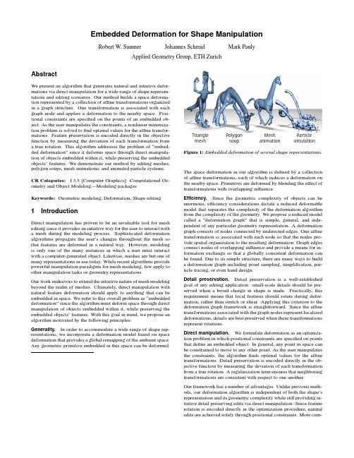
Embedded Deformation for Shape ManipulationRobert W.Sumner Johannes Schmid Mark PaulyApplied Geometry Group,ETH ZurichAbstractWe present an algorithm that generates natural and intuitive defor-mations via direct manipulation for a wide range of shape represen-tations and editing scenarios.Our method builds a space deforma-tion represented by a collection of afﬁne transformations organizedin a graph structure.One transformation is associated with eachgraph node and applies a deformation to the nearby space.Posi-tional constraints are speciﬁed on the points of an embedded ob-ject.As the user manipulates the constraints,a nonlinear minimiza-tion problem is solved toﬁnd optimal values for the afﬁne transfor-mations.Feature preservation is encoded directly in the objective function by measuring the deviation of each transformation from a true rotation.This algorithm addresses the problem of“embed-ded deformation”since it deforms space through direct manipula-tion of objects embedded within it,while preserving the embedded objects’features.We demonstrate our method by editing meshes, polygon soups,mesh animations,and animated particle systems.CR Categories:I.3.5[Computer Graphics]:Computational Ge-ometry and Object Modeling—Modeling packagesKeywords:Geometric modeling,Deformation,Shape editing1IntroductionDirect manipulation has proven to be an invaluable tool for mesh editing since it provides an intuitive way for the user to interact with a mesh during the modeling process.Sophisticated deformation algorithms propagate the user’s changes throughout the mesh so that features are deformed in a natural way.However,modeling is only one of the many instances in which a user must interact with a computer-generated object.Likewise,meshes are but one of many representations in use today.While recent algorithms provide powerful manipulation paradigms for mesh modeling,few apply to other manipulation tasks or geometry representations.Our work endeavors to extend the intuitive nature of mesh modeling beyond the realm of meshes.Ultimately,direct manipulation with natural feature deformation should apply to anything that can be embedded in space.We refer to this overall problem as“embedded deformation”since the algorithm must deform space through direct manipulation of objects embedded within it,while preserving the embedded objects’features.With this goal in mind,we propose an algorithm motivated by the following principles:Generality.In order to accommodate a wide range of shape rep-resentations,we incorporate a deformation model based on space deformation that provides a global remapping of the ambient space. Any geometric primitive embedded in this space can be deformed.PolygonsoupMeshanimationTrianglemeshParticlesimulation Figure1:Embedded deformation of several shape representations.The space deformation in our algorithm is deﬁned by a collection of afﬁne transformations,each of which induces a deformation on the nearby space.Primitives are deformed by blending the effect of transformations with overlapping inﬂuence.Efﬁciency.Since the geometric complexity of objects can be enormous,efﬁciency considerations dictate a reduced deformable model that separates the complexity of the deformation algorithm from the complexity of the geometry.We propose a reduced model called a“deformation graph”that is simple,general,and inde-pendent of any particular geometry representation.A deformation graph consists of nodes connected by undirected edges.One afﬁne transformation is associated with each node so that the nodes pro-vide spatial organization to the resulting deformation.Graph edges connect nodes of overlapping inﬂuence and provide a means for in-formation exchange so that a globally consistent deformation can be found.Due to its simple structure,there are many ways to build a deformation graph including point sampling,simpliﬁcation,par-ticle tracing,or even hand design.Detail preservation.Detail preservation is a well-established goal of any editing application:small-scale details should be pre-served when a broad change in shape is made.Practically,this requirement means that local features should rotate during defor-mation,rather than stretch or shear.Applying this criterion to the deformation graph framework is straightforward.Since the afﬁne transformations associated with the graph nodes represent localized deformations,details are best preserved when these transformations represent rotations.Direct manipulation.We formulate deformation as an optimiza-tion problem in which positional constraints are speciﬁed on points that deﬁne an embedded object.In general,any point in space can be constrained to move to any other point.As the user manipulates the constraints,the algorithmﬁnds optimal values for the afﬁne transformations.Detail preservation is encoded directly in the ob-jective function by measuring the deviation of each transformation from a true rotation.A regularization term ensures that neighboring transformations are consistent with respect to one another.Our framework has a number of advantages.Unlike previous meth-ods,our deformation algorithm is independent of both the shape’s representation and its geometric complexity while still providing in-tuitive detail preserving edits via direct manipulation.Since feature rotation is encoded directly in the optimization procedure,natural edits are achieved solely through positional constraints.More cum-bersome frame transformations are not required.The simplicity and ﬂexibility of the deformation graph make it easy to construct,since a rough distribution of nodes in the region that the user wishes to modify is sufﬁcient.Although the optimization is nonlinear,com-plex edits can be achieved with only a few hundred nodes.Thus, the number of unknowns is small compared to the geometric com-plexity of the embedded object.With our efﬁcient numerical im-plementation,even very detailed shapes can be edited interactively. Our primary contribution is a novel deformation representation and optimization procedure that unites the proven paradigms of direct manipulation and detail preservation with theﬂexibility of space deformations.We highlight the conceptual challenge of embedded deformation and provide a solution that expands intuitive editing to situations where it was previously lacking.Our method accom-modates traditional meshes with multiple connected components, polygon soups,point-based models with no connectivity informa-tion,and mesh animations.Our system also allows the user to in-teractively sculpt the result of a simulated particle system,easily creating effects that would be cumbersome and costly to achieve by tweaking simulation parameters(Figure1).2BackgroundEarly work in shape modeling focuses on space deformations[Barr 1984]that provide a global remapping of space.Free-form defor-mation(FFD)[Sederberg and Parry1988]parameterizes a space deformation with a3D lattice and provides an efﬁcient way to apply coarse deformations to complex shapes.However,achieving aﬁne-scale deformation may require a detailed,hand-designed control lattice[Coquillart1990;MacCracken and Joy1996]and an inordi-nate amount of user manipulation.Although more intuitive control can be provided through direct manipulation[Hsu et al.1992],the user is still restricted by the expressibility of the FFD algorithm. With their“Wires”concept,Singh and Fiume[1998]present aﬂex-ible and effective space deformation algorithm motivated by arma-tures used in traditional sculpting.A collection of space curves tracks deformable features of an object,providing a coarse approx-imation to the shape and a means to deform it.Singh and Kokke-vis[2000]generalize this concept to a polygon-based deformer.In both cases,the user interacts solely with the proxy curves or poly-gons rather than directly with the object being deformed.Rotations, scales,and translations are inferred from the user interaction and applied to the object.These methods give the user powerful tools to design deformations and add detail to a shape.However,they are not well suited to modify shapes that already are highly detailed since the user must design armature curves or control polygons that conform to details at the proper scale in order for the deformation heuristics to generate acceptable results.Due to the widespread availability of very detailed scanned meshes, recent research focuses on high-quality mesh editing through intu-itive user interfaces.Detail preservation is a central goal of such algorithms.Multiresolution methods achieve detail-preserving ed-its at varying scales by generating a hierarchy of simpliﬁed meshes together with corresponding detail coefﬁcients[Kobbelt et al.1998; Botsch and Kobbelt2004].While models with large geometric de-tails may lead to local self-intersections or other artifacts[Botsch et al.2006b],the modeling metaphor presented by Kobbelt and col-leagues[1998]in which a region-of-interest and handle region are deﬁned directly on the mesh is especially notable as it has been applied in nearly every subsequent mesh editing paper. Algorithms based on differential representations extract local shape properties,such as curvature,scale,and orientation.By represent-ing a mesh in terms of these values,editing can be phrased as an energy minimization problem that strives to preserve them[Sorkine 2005].Methods that perform only linear system solves require heuristics or other special treatment of feature rotation,since natu-ral shape deformation is inherently nonlinear[Botsch and Sorkine 2007].V olumetric methods(e.g.,[Zhou et al.2005;Shi et al.2006]) build a dissection of the interior and nearby exterior space for better volume preservation,while subspace methods[Huang et al.2006] build a subspace structure for increased efﬁciency and stability. Nonlinear methods(e.g.,[Sheffer and Kraevoy2004;Huang et al. 2006;Botsch et al.2006a])yield the highest quality edits,although at higher computational costs.These algorithms provide powerful tools for detail-preserving mesh editing.However,these and other mesh editing techniques do not meet the goals of embedded deformation since the deformation al-gorithm is intimately tied to the shape representation.For example, in the method presented by Huang and colleagues[2006],detail preservation is expressed as a mesh-based Laplacian energy that is computed in terms of vertices and their one-ring neighbors.The work of Shi and colleagues[2006]and Zhou and colleagues[2005] both use a Laplacian energy term based on a mesh representation. The prism-based technique of Botsch and colleagues[2006a]uses a deformation energy deﬁned through a coupling of prisms along mesh edges and requires a mesh representation with consistent connectivity.These techniques do not apply to non-meshes,such as point-based representations,particle systems,or polygon soups where no connectivity structure can be assumed.With our method,we adapt the intuitive click-and-drag modeling metaphor used in mesh editing to the context of space deforma-tions.Like Wires[Singh and Fiume1998]and its polygon-based extension[Singh and Kokkevis2000],our method is not tied to one particular representation and can be applied to any primitive de-ﬁned by points in3D.However,unlike Wires or other space defor-mation algorithms that do not explicitly preserve details[Hsu et al. 1992;Botsch and Kobbelt2005],we successfully formulate detail preservation within the space deformation framework.The com-plexity of our deformation graph is independent of the complexity of the shape being edited so that our technique can handle detailed shapes interactively.The graph need not be a volumetric dissec-tion and is simpler to construct than the volumetric or subspace structures used by previous methods.The optimization problem is nonlinear and exhibits comparable quality to nonlinear mesh-based algorithms with less computational cost.Thus,our algorithm com-bines theﬂexibility of space deformations to deform any primitive independent of its geometric complexity with a simple and intuitive click-and-drag interface and high-quality detail preservation.3Deformation GraphThe primary challenge of embedded deformation is toﬁnd a defor-mation model that is general enough to apply to any object embed-ded in space yet still provides intuitive direct manipulation,natural feature preservation,and efﬁciency.We meet these goals with a novel reduced deformable model called a“deformation graph”that can express complex deformations of a variety of shape representa-tions.In this model,a space deformation is deﬁned by a collection of afﬁne transformations.One transformation is associated with each node of a graph embedded in R3,so that the graph provides spatial organization to the deformation.Each afﬁne transformation induces a localized deformation on the nearby space.Undirected edges connect nodes of overlapping inﬂuence to indicate local de-pendencies.The node positions are given by g j∈R3,j∈1...m, and the set N(j)consists of all nodes that share an edge with node j. The afﬁne transformation for node j is speciﬁed by a3×3matrix R j and a3×1translation vector t j.The inﬂuence of the transfor-mation is centered at the node’s position so that it maps any point p in R3to the position˜p according to˜p=R j(p−g j)+g j+t j.(1) A deformed version of the graph itself is computed by applying each afﬁne transformation to its corresponding node.Since g j−g jis the zero vector,the deformed position˜g j of node j is simply equal to g j+t j.More interestingly,the deformation graph can be used to deform any geometric model deﬁned by vertices in R3.Since transfer-ring the deformation to an embedded shape requires computation proportional to the shape’s complexity,efﬁciency is of paramount importance.Consequentially,we employ an algorithm similar to the widely used and highly efﬁcient skeleton-subspace deformation from character animation.The inﬂuence of individual graph nodes is smoothly blended so that the deformed position˜v i of each shape vertex v i,i∈1...n,is a weighted sum of its position after applica-tion of the deformation graph afﬁne transformations:˜v i=m∑j=1w j(v i)R j(v i−g j)+g j+t j.(2)While linear blending may result in some artifacts for extremely coarse graphs,they are negligible for moderately dense ones like those shown in our examples.This result is not surprising,since only a few extra joint transformations are needed to greatly reduce artifacts exhibited by skeleton-subspace deformation[Weber2000; Mohr and Gleicher2003].In our case,the nodes are evenly dis-tributed over the entire shape so that the blended transformations are very similar to one another.Normals are transformed similarly,according to the weighted sum of each normal transformed by the inverse transpose of the node transformations,and then renormalized:˜n i=m∑j=1w j(v i)R−1jn i.(3)The weights w j(v i),j∈1...m,are spatially varying and thus de-pend on the vertex position.Due to the graph structure,transforma-tions that are close to one another will be the most similar.Thus,for consistency and efﬁciency,we limit the inﬂuence of the deforma-tion graph on a particular vertex to the k-nearest nodes.The weights for each vertex are precomputed according tow j(v i)=(1− v i−g j /d max)2(4)and then normalized to sum to one.Here,d max is the distance to the k+1-nearest node.We use k=4for all examples,except the experiment in Figure5(d),where k=8.The layout of the deformation graph nodes should roughly conform to the shape of the model being edited.In our experiments,a uni-form sampling of the model surface produces the best results.Such a sampling is easily accomplished by distributing points densely over the surface,and repeatedly removing all points within a given radius of a randomly chosen one until a desired sampling density is reached.For meshes,simpliﬁcation algorithms also produce good results when the triangle aspect ratio is restricted to avoid long andskinnytriangles.For particle simulations,a simple and efﬁcientconstruction of the node layout can be achieved by sampling parti-cle paths through time.The number of graph nodes determines the expressibility of the deformation graph.Coarse editscan be made with a small number of nodes,while highly detailed ones require denser sampling.Weﬁnd that full body pose changes are effec-tively accomplished with200to300nodes.Graph edges connect nodes of overlapping inﬂuence and are used to enforce consistency in the overall deformation.Once the node po-sitions are determined,the connectivity is computed automatically by creating an edge between any two nodes that inﬂuence the same vertex.Thus,the graph structure depends on how it is evaluated.01234E conE con+E regE con+E reg+E rotR2(g3−g2)+g2+tg2)+g2+t2g2+t2Figure2:A simple deformation graph shows the effect of the three terms of the objective function.The quadrilaterals at each graph node illustrate the deformation induced by the corresponding afﬁne transformation.Without the rotational term,unnatural shearing can occur,as shown in the bottom right.The transformation for node g2is applied to neighboring nodes g1and g3,yielding the predicted positions shown on the bottom left as gray circles.The regularization term minimizes the squared distance between these predicted positions and their actual positions˜g1and˜g3.4OptimizationOnce the deformation graph has been speciﬁed,the user manipu-lates an embedded primitive by selecting vertices and moving them around.The vertices serve as positional constraints for an opti-mization problem in which the afﬁne transformations of the de-formation graph comprise the unknown variables.The objective function encodes detail preservation directly by specifying that the afﬁne transformations should be rotations.Consequently,local fea-tures deform as rigidly as possible.A second energy term serves as a regularizer for the deformation by indicating that the afﬁne trans-formations of adjacent graph nodes should agree with one another. Rotation.In order for a3×3matrix R to represent a rotation in SO(3),it must satisfy six conditions:each of its three columns must be unit length,and all columns must be orthogonal to one an-other[Grassia1998].The squared deviation from these conditions is given by the function Rot(R):Rot(R)=(c1·c2)2+(c1·c3)2+(c2·c3)2+(c1·c1−1)2+(c2·c2−1)2+(c3·c3−1)2(5)where c1,c2,and c3are the3×1column vectors of R.This func-tion is nonlinear in the matrix entries.The term E rot sums the rota-tion error over all transformations of the deformation graph:E rot=m∑j=1Rot(R j).(6)Regularization.Conceptually,each of the afﬁne transformations represents a localized deformation centered at a graph node.Since nearby transformations have overlapping inﬂuence,we must ensure that the computed transformations are consistent with respect to one another.We add a regularization term to the optimization inferred from the graph structure.If nodes j and k are neighbors,they affect a common subset of the embedded shape.The position of node kpredicted by node j’s afﬁne transformation should match the actual position given by applying node k’s transformation to itself(Fig-ure2).The regularization error E reg sums the squared distances between each node’s transformation applied to its neighbors and the actual transformed neighbor positions:E reg=m∑j=1∑k∈N(j)αjkR j(g k−g j)+g j+t j−(g k+t k)22.(7)The weightαjk should be proportional to the degree to which the inﬂuence of nodes j and k overlap.However,the exact amount of overlap is ill deﬁned for many shape representations,such as point-based models and animated particle systems.In order to meet our goal of generality,we useαjk=1.0for all examples.We notice no artifacts compared to experiments using other weighting schemes. This regularization equation bears some resemblance to the defor-mation smoothness energy term used by previous work on template deformation[Allen et al.2003;Sumner and Popovi´c2004;Pauly et al.2005].However,the transformed vertex positions are com-pared,rather than the transformations themselves,and the transfor-mations are relative to the node positions,rather than to the global coordinate system.Constraints.The user controls the optimization through direct manipulation of the embedded shape and need not be aware of the underlying deformation graph.To facilitate editing,our algorithm supports two types of constraints:handle constraints,where a col-lection of model vertices are selected and become handles that are manipulated by the user,andﬁxed constraints,where a collection of model vertices are selected and guaranteed to beﬁxed in place. Handle constraints comprise the interface with which the user in-teracts with an embedded object.These positional constraints are speciﬁed by selecting and moving model vertices.They inﬂuence the optimization since the deformed vertex positions are a function of the graph’s afﬁne transformations.We enforce these constraints using a penalty formulation according to the term E con which is included in the objective function:E con=p∑l=1˜v index(l)−q l22.(8)Vertex˜v index(l)is deformed by the deformation graph according to Eq.2.The vector q l is the user-speciﬁed position of constraint l, and index(l)is the index of the constrained vertex.Fixed constraints are speciﬁed through the same selection mech-anism as handle constraints.However,they are implemented by treating all node transformations that inﬂuence the selected vertices as constants,rather than free variables,and removing them from the optimization procedure.Their primary function is to allow the user to deﬁne the portion of the mesh which is to be edited.Fixed con-straints incur no computational overhead.Conversely,they speed up the computation by reducing the number of unknowns.Thus, the user can make aﬁne-scale edit by using a dense deformation graph and marking all parts of the embedded object not in the edit region asﬁxed.Numerics.Our shape editing framework solves the following op-timization problem:minR1,t1...R m,t mw rot E rot+w reg E reg+w con E con.subject to R q=I,t q=0,∀q∈ﬁxed ids(9)We use the weights w rot=1,w reg=10,and w con=100for all ex-amples.Eq.9is nonlinear in terms of the12m unknowns that deﬁne the afﬁne transformations.Fixed constraints are handled trivially by treating the constrained variables as constants,leaving12m−12q free variables if there are qﬁxed transformations.We implement the iterative Gauss-Newton algorithm to solve the resulting uncon-strained nonlinear least-squares problem[Madsen et al.2004]. The Gauss-Newton algorithm linearizes the nonlinear problem with Taylor expansion about x:f(x+δ)=f(x)+Jδ(10) The vector f(x)stacks the equations that deﬁne the objective func-tion so that f(x) f(x)=F(x)=w rot E rot+w reg E reg+w con E con,the vector x stacks the entries in the afﬁne transformations,and J is the Jacobian matrix of f(x).Each Gauss-Newton iteration solves a lin-earized problem to improve x k,the current estimate of the unknown transformations:δk=argminδf(x k)+Jδ 22x k+1=x k+δk.(11)The process repeats until convergence,which we detect by moni-toring the change in the objective function F k=F(x k),the gradient of the objective function,and the magnitude of the update vectorδk [Gill et al.1989]:|F k−F k−1|<ε(1+F k)∇F k ∞<3√ε(1+F k)(12)δk ∞<2√ε(1+ δk ∞).In our experiments,the optimization converges after about six iter-ations withε=1.0×10−6.In each iteration,we solve the resulting normal equations by Cholesky factorization.Although the linear system J J is very sparse,it depends on x and thus changes at each iteration.There-fore,the full factorization cannot be reused.However,the non-zero structure remains unchanged so that aﬁll-reducing permutation of the matrix and symbolic factorization based only on its non-zero structure can be precomputed and reused[Toledo2003].These steps,together with careful implementation of the routines to build J and J J,result in a very efﬁcient solver.As shown in Table1, each iteration requires about20ms for the presented examples.5ResultsWe have implemented the deformation graph optimization both as an interactive editing application as well as an ofﬂine system for applying scripted constraints to animated data.Live edits with the interactive application are demonstrated in the conference video, and key results are highlighted in this section.Detail preservation.Figure3demonstrates that our algorithm preserves features of the embedded shape.A bumpy plane is mod-iﬁed byﬁxing vertices on the left in place and translating those on the right upward.Although this edit is purely translational,the optimizationﬁnds node transformations that are as close as possi-ble to true rotations while meeting the vertex constraints and main-taining consistency.As a result,the bumps on the plane deform in a natural fashion without shearing artifacts.These results are comparable to the nonlinear prism-based approach of Botsch and colleagues[2006a].However,our algorithm uses a deformation graph of only299nodes,whereas Botsch’s method performs the optimization on the full40,401vertex model and requires a con-sistent meshing of the surface.Figure3also demonstrates that our method preserves details better than the radial-basis function(RBF) approach of Botsch and Kobbelt[2005],where feature rotation is not considered.Figure4demonstrates detail preservation on a more complex exam-ple.With a graph of only222nodes,our approach achieves a defor-mation comparable in quality to the subspace method of Huang andOriginal surface 40,401 vertices Deformation graph299 nodesDeformeddeformation graphDeformed surface PriMo approach of[Botsch et al. 2006]RBF approach of[Botsch & Kobbelt 2005] Figure3:When used to deform a bumpy plane,our method accurately preserves features without shearing or stretching artifacts.The quality of our results is comparable to the“PriMo”approach of Botsch and colleagues[2006a]and superior to the radial-basis function method of Botsch and Kobbelt [2005].Original graphsDeformed graphsDeformed 222 nodes Deformed425 nodesDeformed1,048 nodesOriginalFigure4:We perform an edit similar to the one shown in Figure9 of the work of Huang and colleagues[2006].With a graph of only 222nodes,our results are of comparable quality to Huang’s sub-space gradient domain method.Performing the identical edit with more complex graphs does not yield a signiﬁcant change in quality.colleagues[2006]in which the Laplacian energy is enforced on the full mesh.Higher resolution graphs do not signiﬁcantly improve quality.Performing the same editing task with graphs of425and 1,048nodes yields nearly identical results.Of course,if the graph becomes too sparse to match the complexity of the deformation,ar-tifacts will occur,as can be expected with any reduced deformable model.Likewise,in the highly regular setting shown in Figure5, minor artifacts appear as a slight striped pattern.If additional nodes are used for interpolation or a less regular graph(Figure3),no arti-facts are noticeable.Intuitive editing.Figures6and7demonstrate the intuitive edit-ing framework enabled by our system.High-quality edits are achieved by placing only a handful of single-vertex handle con-straints on the shape.Figure6shows detail-preserving edits on a mesh consisting of85,792vertices.The raptor is deformed by dis-placing positional constraints only,without the need to explicitly specify frame rotations.Fine-scale details such as the teeth and wrinkles are preserved.Furthermore,when the head or body is ma-nipulated and the arms are left unconstrained,the arms rotate in a natural way to follow the body movement.Thus,features are pre-served at a wide range of scales.In this example,a full body pose is sculpted using a graph of226nodes.The tail is lifted,arms crossed, left leg moved forward,and head rotated to look backward.Then, localized changes to the head are made with a more detailed graph of840nodes.However,ﬁxed constraints speciﬁed by selecting the(a)(b)(c)(d)Figure5:A highly regular deformation graph with200nodes, shown in(a),is used to create the deformation in(b).In this struc-tured setting,minor artifacts are visible on the13,024vertex plane, shown in(c),as a slight striped pattern when k=4graph nodes are used for transforming the mesh vertices.These artifacts disappear in(d)when k=8nodes are used and are not present with less struc-tured graphs(Figure3).raptor’s body(green)leave only138active nodes for the head edit so that the system remains interactive.Figure7shows interactive edits on a scanned toy giraffe.The model consists of a set of un-merged range scans that contain many holes and outliers,with a total of79,226vertices in180separate con-nected components.The deformation graph consisting of221nodes is built automatically via uniform sampling,allowing the user to directly edit the shape without time-consuming pre-processing to obtain a consistent mesh representation.Mesh animations.In addition to static geometry,our approach also supports effective editing of dynamic shapes.The mesh anima-tion of Figure8is modiﬁed to lengthen the horse’s legs and neck, and turn its head.The deformation graph,constructed with mesh simpliﬁcation,is advected passively with the animated mesh.Since the graph nodes are chosen to coincide with mesh vertices,no addi-tional computation is required for the node positions to track the an-imation.The user can script edits by setting keyframes on a single pose.Translational offsets are computed from this keyframe data and applied frame-by-frame to the animation sequence with our of-ﬂine application.The graph structure and weighting remainsﬁxed throughout the animation.The output mesh animation incorpo-rates the user’s edits while preserving geometric details,such as the horse’s facial features,as well as high-frequency motion,such as the head bobbing.No multiresolution hierarchy or signal process-ing is needed,unlike the method of Kircher and Garland[2006]. Although we do not address temporal coherence directly,we no-ticed no coherence artifacts in our experiments.Particle simulations.The particle simulation shown in Figure9 is another example of a dynamic shape that can be edited with the deformation graph framework.Our system allows small-scale cor-rections that would be tedious to achieve by tweaking simulation parameters,as well as more drastic modiﬁcations that go beyond the capabilities of a pure simulation.In this example,particle posi-tions are precomputed with aﬂuid simulation.A linear deformation graph is built by sampling the path that a single particle travels over。

英语图标类作文模板范文

英语图标类作文模板范文**English Version****Title: Analyzing and Imitating the English Graphical Essay Template**In the realm of academic writing, the graphical essay, particularly in the context of English, presents a unique challenge. It demands a blend of analytical skills, creativity, and the ability to communicate complex ideas visually. This article aims to explore the structure and content of a popular English graphical essay template and then proceed to create a high-quality imitation.**Structure of the Template:**1. **Introduction:** This section briefly introduces the topic and provides background information. It should end with a clear statement of the purpose of the essay.2. **Description of the Graph/Chart:** Here, the author provides a detailed description of the graph or chart, highlighting key features and patterns.3. **Analysis:** In this section, the author delves deeper into the data, discussing possible reasons behind the trends or patternsobserved. 4. **Discussion:** This part explores the implications of the analysis, relating it to real-world scenarios or theoretical frameworks. 5. **Conclusion:** The essay concludes with a summary of the main points and a closing statement that ties everything together.**High-Quality Imitation of the Template:****Title: Interpreting Trends in Global E-commerce Growth****Introduction:**In recent years, the rise of e-commerce has been nothing short of meteoric. With the advent of technology and the increasing connectivity of the global population, online shopping has become a ubiquitous part of daily life. This essay aims to analyze the growth trends in global e-commerce and explore the factors driving this remarkable transformation.**Description of the Graph:**The provided graph depicts the percentage growth in global e-commerce sales from 2015 to 2025. The x-axis represents the years, while the y-axis represents thepercentage growth. The graph shows a steady increase in e-commerce sales, with a significant jump in recent years.**Analysis:**The consistent growth in global e-commerce sales can be attributed to several factors. Firstly, the widespread availability of high-speed internet and smartphones has made online shopping more accessible and convenient. Secondly, the rise of e-commerce platforms with user-friendly interfaces and a wide range of products has madeit easier for consumers to find and purchase what they need. Additionally, the increasing trust in online payment systems and the provision of secure checkout options have further boosted consumer confidence in online shopping.**Discussion:**The growth trends observed in the graph havesignificant implications for businesses and consumers alike. For businesses, the rise of e-commerce presents a vast opportunity to expand their market reach and connect with a global customer base. However, it also poses challenges, such as the need to adapt to rapidly changing technologies and the increasing competition in the online marketplace.For consumers, the growth of e-commerce means more choices and convenience, but it also raises concerns about data privacy and security.**Conclusion:**In conclusion, the growth trends in global e-commerce are testament to the transformative power of technology and the increasing connectivity of the world. While the rise of e-commerce brings numerous benefits, it also poses challenges that need to be addressed. As we move forward, it will be crucial for businesses and consumers alike to stay abreast of the latest trends and developments in the field of e-commerce.**Chinese Version****标题：英语图表类作文模板解析与仿写**在学术写作领域，图表类作文，尤其是在英语语境下，构成了一个独特的挑战。

基于属性增强的神经传感融合网络的人脸识别算法论文

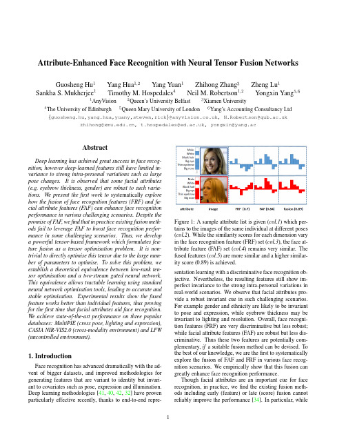
Attribute-Enhanced Face Recognition with Neural Tensor Fusion Networks Guosheng Hu1Yang Hua1,2Yang Yuan1Zhihong Zhang3Zheng Lu1 Sankha S.Mukherjee1Timothy M.Hospedales4Neil M.Robertson1,2Yongxin Yang5,61AnyVision2Queen’s University Belfast3Xiamen University 4The University of Edinburgh5Queen Mary University of London6Yang’s Accounting Consultancy Ltd {guosheng.hu,yang.hua,yuany,steven,rick}@,N.Robertson@ zhihong@,t.hospedales@,yongxin@yang.acAbstractDeep learning has achieved great success in face recog-nition,however deep-learned features still have limited in-variance to strong intra-personal variations such as large pose changes.It is observed that some facial attributes (e.g.eyebrow thickness,gender)are robust to such varia-tions.We present theﬁrst work to systematically explore how the fusion of face recognition features(FRF)and fa-cial attribute features(FAF)can enhance face recognition performance in various challenging scenarios.Despite the promise of FAF,weﬁnd that in practice existing fusion meth-ods fail to leverage FAF to boost face recognition perfor-mance in some challenging scenarios.Thus,we develop a powerful tensor-based framework which formulates fea-ture fusion as a tensor optimisation problem.It is non-trivial to directly optimise this tensor due to the large num-ber of parameters to optimise.To solve this problem,we establish a theoretical equivalence between low-rank ten-sor optimisation and a two-stream gated neural network. This equivalence allows tractable learning using standard neural network optimisation tools,leading to accurate and stable optimisation.Experimental results show the fused feature works better than individual features,thus proving for theﬁrst time that facial attributes aid face recognition. We achieve state-of-the-art performance on three popular databases:MultiPIE(cross pose,lighting and expression), CASIA NIR-VIS2.0(cross-modality environment)and LFW (uncontrolled environment).1.IntroductionFace recognition has advanced dramatically with the ad-vent of bigger datasets,and improved methodologies for generating features that are variant to identity but invari-ant to covariates such as pose,expression and illumination. Deep learning methodologies[41,40,42,32]have proven particularly effective recently,thanks to end-to-endrepre-Figure1:A sample attribute list is given(col.1)which per-tains to the images of the same individual at different poses (col.2).While the similarity scores for each dimension vary in the face recognition feature(FRF)set(col.3),the face at-tribute feature(FAF)set(col.4)remains very similar.The fused features(col.5)are more similar and a higher similar-ity score(0.89)is achieved.sentation learning with a discriminative face recognition ob-jective.Nevertheless,the resulting features still show im-perfect invariance to the strong intra-personal variations in real-world scenarios.We observe that facial attributes pro-vide a robust invariant cue in such challenging scenarios.For example gender and ethnicity are likely to be invariant to pose and expression,while eyebrow thickness may be invariant to lighting and resolution.Overall,face recogni-tion features(FRF)are very discriminative but less robust;while facial attribute features(FAF)are robust but less dis-criminative.Thus these two features are potentially com-plementary,if a suitable fusion method can be devised.To the best of our knowledge,we are theﬁrst to systematically explore the fusion of FAF and FRF in various face recog-nition scenarios.We empirically show that this fusion can greatly enhance face recognition performance.Though facial attributes are an important cue for face recognition,in practice,weﬁnd the existing fusion meth-ods including early(feature)or late(score)fusion cannot reliably improve the performance[34].In particular,while 1offering some robustness,FAF is generally less discrimina-tive than FRF.Existing methods cannot synergistically fuse such asymmetric features,and usually lead to worse perfor-mance than achieved by the stronger feature(FRF)only.In this work,we propose a novel tensor-based fusion frame-work that is uniquely capable of fusing the very asymmet-ric FAF and FRF.Our framework provides a more powerful and robust fusion approach than existing strategies by learn-ing from all interactions between the two feature views.To train the tensor in a tractable way given the large number of required parameters,we formulate the optimisation with an identity-supervised objective by constraining the tensor to have a low-rank form.We establish an equivalence be-tween this low-rank tensor and a two-stream gated neural network.Given this equivalence,the proposed tensor is eas-ily optimised with standard deep neural network toolboxes. Our technical contributions are:•It is theﬁrst work to systematically investigate and ver-ify that facial attributes are an important cue in various face recognition scenarios.In particular,we investi-gate face recognition with extreme pose variations,i.e.±90◦from frontal,showing that attributes are impor-tant for performance enhancement.•A rich tensor-based fusion framework is proposed.We show the low-rank Tucker-decomposition of this tensor-based fusion has an equivalent Gated Two-stream Neural Network(GTNN),allowing easy yet effective optimisation by neural network learning.In addition,we bring insights from neural networks into theﬁeld of tensor optimisation.The code is available:https:///yanghuadr/ Neural-Tensor-Fusion-Network•We achieve state-of-the-art face recognition perfor-mance using the fusion of face(newly designed‘Lean-Face’deep learning feature)and attribute-based fea-tures on three popular databases:MultiPIE(controlled environment),CASIA NIR-VIS2.0(cross-modality environment)and LFW(uncontrolled environment).2.Related WorkFace Recognition.The face representation(feature)is the most important component in contemporary face recog-nition system.There are two types:hand-crafted and deep learning features.Widely used hand-crafted face descriptors include Local Binary Pattern(LBP)[26],Gaborﬁlters[23],-pared to pixel values,these features are variant to identity and relatively invariant to intra-personal variations,and thus they achieve promising performance in controlled environ-ments.However,they perform less well on face recognition in uncontrolled environments(FRUE).There are two main routes to improve FRUE performance with hand-crafted features,one is to use very high dimensional features(dense sampling features)[5]and the other is to enhance the fea-tures with downstream metric learning.Unlike hand-crafted features where(in)variances are en-gineered,deep learning features learn the(in)variances from data.Recently,convolutional neural networks(CNNs) achieved impressive results on FRUE.DeepFace[44],a carefully designed8-layer CNN,is an early landmark method.Another well-known line of work is DeepID[41] and its variants DeepID2[40],DeepID2+[42].The DeepID family uses an ensemble of many small CNNs trained in-dependently using different facial patches to improve the performance.In addition,some CNNs originally designed for object recognition,such as VGGNet[38]and Incep-tion[43],were also used for face recognition[29,32].Most recently,a center loss[47]is introduced to learn more dis-criminative features.Facial Attribute Recognition.Facial attribute recog-nition(FAR)is also well studied.A notable early study[21] extracted carefully designed hand-crafted features includ-ing aggregations of colour spaces and image gradients,be-fore training an independent SVM to detect each attribute. As for face recognition,deep learning features now outper-form hand-crafted features for FAR.In[24],face detection and attribute recognition CNNs are carefully designed,and the output of the face detection network is fed into the at-tribute network.An alternative to purpose designing CNNs for FAR is toﬁne-tune networks intended for object recog-nition[56,57].From a representation learning perspective, the features supporting different attribute detections may be shared,leading some studies to investigate multi-task learn-ing facial attributes[55,30].Since different facial attributes have different prevalence,the multi-label/multi-task learn-ing suffers from label-imbalance,which[30]addresses us-ing a mixed objective optimization network(MOON). Face Recognition using Facial Attributes.Detected facial attributes can be applied directly to authentication. Facial attributes have been applied to enhance face veriﬁca-tion,primarily in the case of cross-modal matching,byﬁl-tering[19,54](requiring potential FRF matches to have the correct gender,for example),model switching[18],or ag-gregation with conventional features[27,17].[21]deﬁnes 65facial attributes and proposes binary attribute classiﬁers to predict their presence or absence.The vector of attribute classiﬁer scores can be used for face recognition.There has been little work on attribute-enhanced face recognition in the context of deep learning.One of the few exploits CNN-based attribute features for authentication on mobile devices [31].Local facial patches are fed into carefully designed CNNs to predict different attributes.After CNN training, SVMs are trained for attribute recognition,and the vector of SVM scores provide the new feature for face veriﬁcation.Fusion Methods.Existing fusion approaches can be classiﬁed into feature-level(early fusion)and score-level (late fusion).Score-level fusion is to fuse the similarity scores after computation based on each view either by sim-ple averaging[37]or stacking another classiﬁer[48,37]. Feature-level fusion can be achieved by either simple fea-ture aggregation or subspace learning.For aggregation ap-proaches,fusion is usually performed by simply element wise averaging or product(the dimension of features have to be the same)or concatenation[28].For subspace learn-ing approaches,the features areﬁrst concatenated,then the concatenated feature is projected to a subspace,in which the features should better complement each other.These sub-space approaches can be unsupervised or supervised.Un-supervised fusion does not use the identity(label)informa-tion to learn the subspace,such as Canonical Correlational Analysis(CCA)[35]and Bilinear Models(BLM)[45].In comparison,supervised fusion uses the identity information such as Linear Discriminant Analysis(LDA)[3]and Local-ity Preserving Projections(LPP)[9].Neural Tensor Methods.Learning tensor-based compu-tations within neural networks has been studied for full[39] and decomposed[16,52,51]tensors.However,aside from differing applications and objectives,the key difference is that we establish a novel equivalence between a rich Tucker [46]decomposed low-rank fusion tensor,and a gated two-stream neural network.This allows us achieve expressive fusion,while maintaining tractable computation and a small number of parameters;and crucially permits easy optimisa-tion of the fusion tensor through standard toolboxes. Motivation.Facial attribute features(FAF)and face recognition features(FRF)are complementary.However in practice,weﬁnd that existing fusion methods often can-not effectively combine these asymmetric features so as to improve performance.This motivates us to design a more powerful fusion method,as detailed in Section3.Based on our neural tensor fusion method,in Section5we system-atically explore the fusion of FAF and FRF in various face recognition environments,showing that FAF can greatly en-hance recognition performance.3.Fusing attribute and recognition featuresIn this section we present our strategy for fusing FAF and FRF.Our goal is to input FAF and FRF and output the fused discriminative feature.The proposed fusion method we present here performs signiﬁcantly better than the exist-ing ones introduced in Section2.In this section,we detail our tensor-based fusion strategy.3.1.ModellingSingle Feature.We start from a standard multi-class clas-siﬁcation problem setting:assume we have M instances, and for each we extract a D-dimensional feature vector(the FRF)as{x(i)}M i=1.The label space contains C unique classes(person identities),so each instance is associated with a corresponding C-dimensional one-hot encoding la-bel vector{y(i)}M i=1.Assuming a linear model W the pre-dictionˆy(i)is produced by the dot-product of input x(i)and the model W,ˆy(i)=x(i)T W.(1) Multiple Feature.Suppose that apart from the D-dimensional FRF vector,we can also obtain an instance-wise B-dimensional facial attribute feature z(i).Then the input for the i th instance is a pair:{x(i),z(i)}.A simple ap-proach is to redeﬁne x(i):=[x(i),z(i)],and directly apply Eq.(1),thus modelling weights for both FRF and FAF fea-tures.Here we propose instead a non-linear fusion method via the following formulationˆy(i)=W×1x(i)×3z(i)(2) where W is the fusion model parameters in the form of a third-order tensor of size D×C×B.Notation×is the tensor dot product(also known as tensor contraction)and the left-subscript of x and z indicates at which axis the ten-sor dot product operates.With Eq.(2),the optimisation problem is formulated as:minW1MMi=1W×1x(i)×3z(i),y(i)(3)where (·,·)is a loss function.This trains tensor W to fuse FRF and FAF features so that identity is correctly predicted.3.2.OptimisationThe proposed tensor W provides a rich fusion model. However,compared with W,W is B times larger(D×C vs D×C×B)because of the introduction of B-dimensional attribute vector.It is also almost B times larger than train-ing a matrix W on the concatenation[x(i),z(i)].It is there-fore problematic to directly optimise Eq.(3)because the large number of parameters of W makes training slow and leads to overﬁtting.To address this we propose a tensor de-composition technique and a neural network architecture to solve an equivalent optimisation problem in the following two subsections.3.2.1Tucker Decomposition for Feature FusionTo reduce the number of parameters of W,we place a struc-tural constraint on W.Motivated by the famous Tucker de-composition[46]for tensors,we assume that W is synthe-sised fromW=S×1U(D)×2U(C)×3U(B).(4) Here S is a third order tensor of size K D×K C×K B, U(D)is a matrix of size K D×D,U(C)is a matrix of sizeK C×C,and U(B)is a matrix of size K B×B.By restricting K D D,K C C,and K B B,we can effectively reduce the number of parameters from(D×C×B)to (K D×K C×K B+K D×D+K C×C+K B×B)if we learn{S,U(D),U(C),U(B)}instead of W.When W is needed for making the predictions,we can always synthesise it from those four small factors.In the context of tensor decomposition,(K D,K C,K B)is usually called the tensor’s rank,as an analogous concept to the rank of a matrix in matrix decomposition.Note that,despite of the existence of other tensor de-composition choices,Tucker decomposition offers a greater ﬂexibility in terms of modelling because we have three hyper-parameters K D,K C,K B corresponding to the axes of the tensor.In contrast,the other famous decomposition, CP[10]has one hyper-parameter K for all axes of tensor.By substituting Eq.(4)into Eq.(2),we haveˆy(i)=W×1x(i)×3z(i)=S×1U(D)×2U(C)×3U(B)×1x(i)×3z(i)(5) Through some re-arrangement,Eq.(5)can be simpliﬁed as ˆy(i)=S×1(U(D)x(i))×2U(C)×3(U(B)z(i))(6) Furthermore,we can rewrite Eq.(6)as,ˆy(i)=((U(D)x(i))⊗(U(B)z(i)))S T(2)fused featureU(C)(7)where⊗is Kronecker product.Since U(D)x(i)and U(B)B(i)result in K D and K B dimensional vectors re-spectively,(U(D)x(i))⊗(U(B)z(i))produces a K D K B vector.S(2)is the mode-2unfolding of S which is aK C×K D K B matrix,and its transpose S T(2)is a matrix ofsize K D K B×K C.The Fused Feature.From Eq.(7),the explicit fused representation of face recognition(x(i))and facial at-tribute(z(i))features can be achieved.The fused feature ((U(D)x(i))⊗(U(B)z(i)))S T(2),is a vector of the dimen-sionality K C.And matrix U(C)has the role of“clas-siﬁer”given this fused feature.Given{x(i),z(i),y(i)}, the matrices{U(D),U(B),U(C)}and tensor S are com-puted(learned)during model optimisation(training).Dur-ing testing,the predictionˆy(i)is achieved with the learned {U(D),U(B),U(C),S}and two test features{x(i),z(i)} following Eq.(7).3.2.2Gated Two-stream Neural Network(GTNN)A key advantage of reformulating Eq.(5)into Eq.(7)is that we can nowﬁnd a neural network architecture that does ex-actly the computation of Eq.(7),which would not be obvi-ous if we stopped at Eq.(5).Before presenting thisneural Figure2:Gated two-stream neural network to implement low-rank tensor-based fusion.The architecture computes Eq.(7),with the Tucker decomposition in Eq.(4).The network is identity-supervised at train time,and feature in the fusion layer used as representation for veriﬁcation. network,we need to introduce a new deterministic layer(i.e. without any learnable parameters).Kronecker Product Layer takes two arbitrary-length in-put vectors{u,v}where u=[u1,u2,···,u P]and v=[v1,v2,···,v Q],then outputs a vector of length P Q as[u1v1,u1v2,···,u1v Q,u2v1,···,u P v Q].Using the introduced Kronecker layer,Fig.2shows the neural network that computes Eq.(7).That is,the neural network that performs recognition using tensor-based fu-sion of two features(such as FAF and FRF),based on the low-rank assumption in Eq.(4).We denote this architecture as a Gated Two-stream Neural Network(GTNN),because it takes two streams of inputs,and it performs gating[36] (multiplicative)operations on them.The GTNN is trained in a supervised fashion to predict identity.In this work,we use a multitask loss:softmax loss and center loss[47]for joint training.The fused feature in the viewpoint of GTNN is the output of penultimate layer, which is of dimensionality K c.So far,the advantage of using GTNN is obvious.Direct use of Eq.(5)or Eq.(7)requires manual derivation and im-plementation of an optimiser which is non-trivial even for decomposed matrices(2d-tensors)[20].In contrast,GTNN is easily implemented with modern deep learning packages where auto-differentiation and gradient-based optimisation is handled robustly and automatically.3.3.DiscussionCompared with the fusion methods introduced in Sec-tion2,we summarise the advantages of our tensor-based fusion method as follows:Figure3:LeanFace.‘C’is a group of convolutional layers.Stage1:64@5×5(64feature maps are sliced to two groups of32ones, which are fed into maxout function.);Stage2:64@3×3,64@3×3,128@3×3,128@3×3;Stage3:196@3×3,196@3×3, 256@3×3,256@3×3,320@3×3,320@3×3;Stage4:512@3×3,512@3×3,512@3×3,512@3×3;Stage5:640@ 5×5,640@5×5.‘P’stands for2×2max pooling.The strides for the convolutional and pooling layers are1and2,respectively.‘FC’is a fully-connected layer of256D.High Order Non-Linearity.Unlike linear methods based on averaging,concatenation,linear subspace learning [8,27],or LDA[3],our fusion method is non-linear,which is more powerful to model complex problems.Further-more,comparing with otherﬁrst-order non-linear methods based on element-wise combinations only[28],our method is higher order:it accounts for all interactions between each pair of feature channels in both views.Thanks to the low-rank modelling,our method achieves such powerful non-linear fusion with few parameters and thus it is robust to overﬁtting.Scalability.Big datasets are required for state-of-the-art face representation learning.Because we establish the equivalence between tensor factorisation and gated neural network architecture,our method is scalable to big-data through efﬁcient mini-batch SGD-based learning.In con-trast,kernel-based non-linear methods,such as Kernel LDA [34]and multi-kernel SVM[17],are restricted to small data due to their O(N2)computation cost.At runtime,our method only requires a simple feed-forward pass and hence it is also favourable compared to kernel methods. Supervised method.GTNN isﬂexibly supervised by any desired neural network loss function.For example,the fusion method can be trained with losses known to be ef-fective for face representation learning:identity-supervised softmax,and centre-loss[47].Alternative methods are ei-ther unsupervised[8,27],constrained in the types of super-vision they can exploit[3,17],or only stack scores rather than improving a learned representation[48,37].There-fore,they are relatively ineffective at learning how to com-bine the two-source information in a task-speciﬁc way. Extensibility.Our GTNN naturally can be extended to deeper architectures.For example,the pre-extracted fea-tures,i.e.,x and z in Fig.2,can be replaced by two full-sized CNNs without any modiﬁcation.Therefore,poten-tially,our methods can be integrated into an end-to-end framework.4.Integration with CNNs:architectureIn this section,we introduce the CNN architectures used for face recognition(LeanFace)designed by ourselves and facial attribute recognition(AttNet)introduced by[50,30]. LeanFace.Unlike general object recognition,face recognition has to capture very subtle difference between people.Motivated by theﬁne-grain object recognition in [4],we also use a large number of convolutional layers at early stage to capture the subtle low level and mid-level in-formation.Our activation function is maxout,which shows better performance than its competitors[50].Joint supervi-sion of softmax loss and center loss[47]is used for training. The architecture is summarised in Fig.3.AttNet.To detect facial attributes,our AttNet uses the ar-chitecture of Lighten CNN[50]to represent a face.Speciﬁ-cally,AttNet consists of5conv-activation-pooling units fol-lowed by a256D fully connected layer.The number of con-volutional kernels is explained in[50].The activation func-tion is Max-Feature-Map[50]which is a variant of maxout. We use the loss function MOON[30],which is a multi-task loss for(1)attribute classiﬁcation and(2)domain adaptive data balance.In[24],an ontology of40facial attributes are deﬁned.We remove attributes which do not characterise a speciﬁc person,e.g.,‘wear glasses’and‘smiling’,leaving 17attributes in total.Once each network is trained,the features extracted from the penultimate fully-connected layers of LeanFace(256D) and AttNet(256D)are extracted as x and z,and input to GTNN for fusion and then face recognition.5.ExperimentsWeﬁrst introduce the implementation details of our GTNN method.In Section5.1,we conduct experiments on MultiPIE[7]to show that facial attributes by means of our GTNN method can play an important role on improv-Table1:Network training detailsImage size BatchsizeLR1DF2EpochTraintimeLeanFace128x1282560.0010.15491hAttNet0.050.8993h1Learning rate(LR)2Learning rate drop factor(DF).ing face recognition performance in the presence of pose, illumination and expression,respectively.Then,we com-pare our GTNN method with other fusion methods on CA-SIA NIR-VIS2.0database[22]in Section5.2and LFW database[12]in Section5.3,respectively. Implementation Details.In this study,three networks (LeanFace,AttNet and GTNN)are discussed.LeanFace and AttNet are implemented using MXNet[6]and GTNN uses TensorFlow[1].We use around6M training face thumbnails covering62K different identities to train Lean-Face,which has no overlapping with all the test databases. AttNet is trained using CelebA[24]database.The input of GTNN is two256D features from bottleneck layers(i.e., fully connected layers before prediction layers)of LeanFace and AttNet.The setting of main parameters are shown in Table1.Note that the learning rates drop when the loss stops decreasing.Speciﬁcally,the learning rates change4 and2times for LeanFace and AttNet respectively.Dur-ing test,LeanFace and AttNet take around2.9ms and3.2ms to extract feature from one input image and GTNN takes around2.1ms to fuse one pair of LeanFace and AttNet fea-ture using a GTX1080Graphics Card.5.1.Multi-PIE DatabaseMulti-PIE database[7]contains more than750,000im-ages of337people recorded in4sessions under diverse pose,illumination and expression variations.It is an ideal testbed to investigate if facial attribute features(FAF) complement face recognition features(FRF)including tra-ditional hand-crafted(LBP)and deeply learned features (LeanFace)to improve the face recognition performance–particularly across extreme pose variation.Settings.We conduct three experiments to investigate pose-,illumination-and expression-invariant face recogni-tion.Pose:Uses images across4sessions with pose vari-ations only(i.e.,neutral lighting and expression).It covers pose with yaw ranging from left90◦to right90◦.In com-parison,most of the existing works only evaluate perfor-mance on poses with yaw range(-45◦,+45◦).Illumination: Uses images with20different illumination conditions(i.e., frontal pose and neutral expression).Expression:Uses im-ages with7different expression variations(i.e.,frontal pose and neutral illumination).The training sets of all settings consist of the images from theﬁrst200subjects and the re-maining137subjects for testing.Following[59,14],in the test set,frontal images with neural illumination and expres-sion from the earliest session work as gallery,and the others are probes.Pose.Table2shows the pose-robust face recognition (PRFR)performance.Clearly,the fusion of FRF and FAF, namely GTNN(LBP,AttNet)and GTNN(LeanFace,At-tNet),works much better than using FRF only,showing the complementary power of facial features to face recognition features.Not surprisingly,the performance of both LBP and LeanFace features drop greatly under extreme poses,as pose variation is a major factor challenging face recognition performance.In contrast,with GTNN-based fusion,FAF can be used to improve both classic(LBP)and deep(Lean-Face)FRF features effectively under this circumstance,for example,LBP(1.3%)vs GTNN(LBP,AttNet)(16.3%), LeanFace(72.0%)vs GTNN(LeanFace,AttNet)(78.3%) under yaw angel−90◦.It is noteworthy that despite their highly asymmetric strength,GTNN is able to effectively fuse FAF and FRF.This is elaborately studied in more detail in Sections5.2-5.3.Compared with state-of-the-art methods[14,59,11,58, 15]in terms of(-45◦,+45◦),LeanFace achieves better per-formance due to its big training data and the strong gener-alisation capacity of deep learning.In Table2,2D meth-ods[14,59,15]trained models using the MultiPIE images, therefore,they are difﬁcult to generalise to images under poses which do not appear in MultiPIE database.3D meth-ods[11,58]highly depend on accurate2D landmarks for 3D-2D modellingﬁtting.However,it is hard to accurately detect such landmarks under larger poses,limiting the ap-plications of3D methods.Illumination and expression.Illumination-and expression-robust face recognition(IRFR and ERFR)are also challenging research topics.LBP is the most widely used handcrafted features for IRFR[2]and ERFR[33].To investigate the helpfulness of facial attributes,experiments of IRFR and ERFR are conducted using LBP and Lean-Face features.In Table3,GTNN(LBP,AttNet)signiﬁ-cantly outperforms LBP,80.3%vs57.5%(IRFR),77.5% vs71.7%(ERFR),showing the great value of combining fa-cial attributes with hand-crafted features.Attributes such as the shape of eyebrows are illumination invariant and others, e.g.,gender,are expression invariant.In contrast,LeanFace feature is already very discriminative,saturating the perfor-mance on the test set.So there is little room for fusion of AttrNet to provide beneﬁt.5.2.CASIA NIR-VIS2.0DatabaseThe CASIA NIR-VIS2.0face database[22]is the largest public face database across near-infrared(NIR)images and visible RGB(VIS)images.It is a typical cross-modality or heterogeneous face recognition problem because the gallery and probe images are from two different spectra.The。

image alignment and stitching a tutorial

Image Alignment and Stitching: A Tutorial1
Richard Szeliski Last updated, December 10, 2006 Technical Report MSR-TR-2004-92
This tutorial reviews image alignment and image stitching algorithms. Image alignment algorithms can discover the correspondence relationships among images with varying degrees of overlap. They are ideally suited for applications such as video stabilization, summarization, and the creation of panoramic mosaics. Image stitching algorithms take the alignment estimates produced by such registration algorithms and blend the images in a seamless manner, taking care to deal with potential problems such as blurring or ghosting caused by parallax and scene movement as well as varying image exposures. This tutorial reviews the basic motion models underlying alignment and stitching algorithms, describes effective direct (pixel-based) and feature-based alignment algorithms, and describes blending algorithms used to produce seamless mosaics. It closes with a discussion of open research problems in the area.

Graph rewriting

Graph rewritingGraph transformation,or graph rewriting,concerns the technique of creating a new graph out of an origi-nal graph algorithmically.It has numerous applications, ranging from software engineering(software construction and also software veriﬁcation)to layout algorithms and picture generation.Graph transformations can be used as a computation ab-straction.The basic idea is that the state of a computa-tion can be represented as a graph,further steps in that computation can then be represented as transformation rules on that graph.Such rules consist of an original graph,which is to be matched to a subgraph in the com-plete state,and a replacing graph,which will replace the matched subgraph.Formally,a graph rewriting system usually consists of a set of graph rewrite rules of the form L→R,with L being called pattern graph(or left-hand side)and R be-ing called replacement graph(or right-hand side of the rule).A graph rewrite rule is applied to the host graph by searching for an occurrence of the pattern graph(pattern matching,thus solving the subgraph isomorphism prob-lem)and by replacing the found occurrence by an instance of the replacement graph.Rewrite rules can be further regulated in the case of labeled graphs,such as in string-regulated graph grammars.Sometimes graph grammar is used as a synonym for graph rewriting system,especially in the context of formal languages;the diﬀerent wording is used to em-phasize the goal of constructions,like the enumeration of all graphs from some starting graph,i.e.the generation of a graph language–instead of simply transforming a given state(host graph)into a new state.1Graph rewriting approaches There are several approaches to graph rewriting.One of them is the algebraic approach,which is based upon category theory.The algebraic approach is divided into some sub approaches,the double-pushout(DPO)ap-proach and the single-pushout(SPO)approach being the most common ones;further on there are the sesqui-pushout and the pullback approach.From the perspective of the DPO approach a graph rewriting rule is a pair of morphisms in the category of graphs with total graph morphisms as arrows:r=(L←K→R)(or L⊇K⊆R)where K→L is injective. The graph K is called invariant or sometimes the gluinggraph.A rewriting step or application of a rule r to a host graph G is deﬁned by two pushout diagrams both origi-nating in the same morphism k:K→G(this is where the name double-pushout comes from).Another graph morphism m:L→G models an occurrence of L in G and is called a match.Practical understanding of this is that L is a subgraph that is matched from G(see subgraph isomorphism problem),and after a match is found,L is replaced with R in host graph G where K serves as an interface,containing the nodes and edges which are pre-served when applying the rule.The graph K is needed to attach the pattern being matched to its context:if it is empty,the match can only designate a whole connected component of the graph G.In contrast a graph rewriting rule of the SPO approach is a single morphism in the category labeled multigraphs with partial graph morphisms as arrows:r:L→R. Thus a rewriting step is deﬁned by a single pushout di-agram.Practical understanding of this is similar to the DPO approach.The diﬀerence is,that there is no inter-face between the host graph G and the graph G'being the result of the rewriting step.There is also another algebraic-like approach to graph rewriting,based mainly on Boolean algebra and an alge-bra of matrices,called matrix graph grammars.[1][2] Yet another approach to graph rewriting,known as deter-minate graph rewriting,came out of logic and database theory.In this approach,graphs are treated as database instances,and rewriting operations as a mechanism for deﬁning queries and views;therefore,all rewriting is re-quired to yield unique results(up to isomorphism),and this is achieved by applying any rewriting rule concur-rently throughout the graph,wherever it applies,in such a way that the result is indeed uniquely deﬁned.2Term graph rewritingAnother approach to graph rewriting is term graph rewrit-ing,which involves the processing or transformation of term graphs(also known as abstract semantic graphs)by a set of syntactic rewrite rules.Term graphs are a prominent topic in programming lan-guage research since term graph rewriting rules are ca-pable of formally expressing a compiler’s operational se-mantics.Term graphs are also used as abstract machines capable of modelling chemical and biological compu-tations as well as graphical calculi such as concurrency 123IMPLEMENTATIONS AND APPLICATIONSmodels.Term graphs can perform automated veriﬁca-tion and logical programming since they are well-suited to representing quantiﬁed statements in ﬁrst order logic.Symbolic programming software is another application for term graphs,which are capable of representing and performing computation with abstract algebraic struc-tures such as groups,ﬁelds and rings.The TERMGRAPH conference [3]focuses entirely on re-search into term graph rewriting and its applications.3Implementations and applica-tionsExample for graph rewrite rule (optimization from compiler con-struction:multiplication with 2replaced by addition)Graphs are an expressive,visual and mathematically pre-cise formalism for modelling of objects (entities)linked by relations;objects are represented by nodes and rela-tions between them by edges.Nodes and edges are com-monly typed and putations are described in this model by changes in the relations between the en-tities or by attribute changes of the graph elements.They are encoded in graph rewrite/graph transformation rules and executed by graph rewrite systems/graph transforma-tion tools.•Tools that are application domain neutral:• ,the graph rewrite generator,a graph transformation tool emitting C#-code or .NET-assemblies•AGG ,the attributed graph grammar system (Java )•GP (Graph Programs)is a programming lan-guage for computing on graphs by the directed application of graph transformation rules.•GMTE ,the Graph Matching and Transforma-tion Engine for graph matching and transfor-mation.It is an implementation of an exten-sion of Messmer’s algorithm using C++.•GROOVE ,a Java-based tool set for editing graphs and graph transformation rules,explor-ing the state spaces of graph grammars,and model checking those state spaces;can also be used as a graph transformation engine.•Tools that solve software engineering tasks (mainly MDA )with graph rewriting:•eMoﬂon ,an EMF-compliant model-transformation tool with support for Story-Driven Modeling and Triple Graph Grammars •GReAT •VIATRA•Graph databases often support dynamic rewriting of graphs•Gremlin ,a graph-based programming lan-guage (see Graph Rewriting )•PROGRES ,an integrated environment and very high level language for PROgrammed Graph REwriting Systems•Fujaba uses Story driven modelling,a graph rewrite language based on PROGRES •EMorF and Henshin ,graph rewriting systems based on EMF ,supporting in-place model transformation and model to model transfor-mation•Mechanical engineering tools•GraphSynth is an interpreter and UI environ-ment for creating unrestricted graph grammars as well as testing and searching the resultant language variant.It saves graphs and graph grammar rules as XML ﬁles and is written in C#.•Soley Studio ,is an integrated development en-vironment for graph transformation systems.It’s main application focus is data analytics in the ﬁeld of engineering.•Biology applications•Functional-structural plant modeling with a graph grammar based language•Multicellular development modeling with string-regulated graph grammars•Artiﬁcial Intelligence/Natural Language Processing•OpenCog provides a basic pattern matcher (on hypergraphs )which is used to implement var-ious AI algorithms.3•RelEx is an English-language parser that em-ploys graph re-writing to convert a link parseinto a dependency parse.4See also•Category theory•Graph theory•Shape grammar•Term graph5Notes[1]Perez2009covers this approach in detail.[2]This topic is expanded at .[3]“TERMGRAPH”.6References•Rozenberg,Grzegorz(1997),Handbook of GraphGrammars and Computing by Graph Transforma-tions,World Scientiﬁc Publishing,volumes1–3,ISBN9810228848.•Perez,P.P.(2009),Matrix Graph Grammars:An Al-gebraic Approach to Graph Dynamics,VDM Verlag,ISBN978-3-639-21255-6.•Heckel,R.(2006).Graph transformation in a nut-shell.Electronic Notes in Theoretical ComputerScience148(1SPEC.ISS.),pp.187–198.•König,Barbara(2004).Analysis and Veriﬁca-tion of Systems with Dynamically Evolving Structure.Habilitation thesis,Universität Stuttgart,pp.65–180.•Lobo,D.et al.(2011).Graph grammars with string-regulated rewriting.Theoretical Computer Science,412(43),pp.6101-6111.47TEXT AND IMAGE SOURCES,CONTRIBUTORS,AND LICENSES 7Text and image sources,contributors,and licenses7.1Text•Graph rewriting Source:/wiki/Graph%20rewriting?oldid=651791188Contributors:Rp,Silverﬁsh,MathMartin, Giftlite,Thv,Matt Crypto,Cmdrjameson,R.S.Shaw,Oleg Alexandrov,Linas,Rjwilmsi,Batztown,Michael Slone,Arthur Rubin,Rtc, Dougher,David Eppstein,Ppablo1812,Addbot,JakobVoss,4th-otaku,AnomieBOT,Gragragra,HanielBarbosa,TechBot,Mattica,2nd-jpeg,FrescoBot,Gwpl,Playmobilonhishorse,Waidanian,Ɯ,Ptrb,Helpful Pixie Bot,Bouassida,Eptiﬁed,Loelib,Mark viking,Dokkam, RolandKluge and Anonymous:377.2Images•File:GraphRewriteExample.PNG Source:/wikipedia/commons/4/44/GraphRewriteExample.PNG License: Public domain Contributors:Own work Original artist:Gragra7.3Content license•Creative Commons Attribution-Share Alike3.0。

冰花曲线的发明者：冰花曲线的真正起源说明书

WHO INVENTED VON KOCH’S SNOWFLAKE CUR VE?YANN DEMICHEL †Abstract.A strange title,might you say:Answer is in the question!However,contrary to popular belief and numerous citations in the literature,the image of the snowflake curve is not present or even mentioned in von Koch’s original articles.So,where and when did the first snowflake fall?Unravel the mystery of the snowflake curve with us on a journey through time.Introduction In 2024we will commemorate the centenary of the death of Swedish mathematician Helge von Koch.We will also be celebrating the 120th anniversary of the birth of its famous curve.Less well known,von Koch was part of the first generation of mathematicians around Mittag-Leffler at the newly created Stockholms H¨o gskola (see [7]).While most of his work is now outdated,his name has gone down in history for having been given to one of the most emblematic geometric figures of the 20th century:the snowflake curve.Known for its a priori paradoxical property of possessing an infinite perimeter but delimiting a finite area,it owes its fame to its suggestive and particularly aesthetic shape.Yet a mystery remains.The snowflake curve is clearly based on von Koch’s construction but it does not appear in either the original 1904article or the extended 1906version (see [10,11]).In fact,it does not appear in any of the Swedish mathematician’s works.So,who is behind the snowflake curve?When and where did it first appear?That is what we will try to find out. 1.Follow tracks in the snow The starting point of our investigation is von Koch’s native Sweden.Chosen as the emblem of the Swedish Mathematical Society,the snowflake curve is the pride of the profession.In 2000,declared the World Mathematical Year,the Swedish Post Office honored it for Christmas celebration.Two stamps featuring the snowflake are issued,affixed to an envelope showing the first stages of the snowflake construction,and canceled with a special postmark (see Figure 1).The stamps are marked Helge von Kochs sn¨o flingekurva and the back of the envelope reads:“In 1904the Swedish mathematician Helge von Koch (1870–1924)constructedan early example of fractals,the snowflake curve.”Not surprisingly Sweden fully claims the property of the figure and its inventor,and invites us to follow the path of fractal geometry.A few years earlier it was in this context that the snowflake was twice the star of the science pages of the national daily newspaper Svenska Dagbladet (see[3,4]).In 1991it shared the bill with the original curve,demonstrating its obvious kinship.Two versions of the same curve,both attributed to von Koch.In the 1983article,it is presented as the archetypal image of the new geometry developed by Benoˆıt Mandelbrot.2020Mathematics Subject Classification.01A60,01A70,28A80.Key words and phrases.Snowflake curve,von Koch curve,Helge von Koch,Fractal curve.1a r X i v :2308.15093v 1 [m a t h .H O ] 29 A u g 20232YANN DEMICHELFigure1.The limited-edition First Day Cover envelope printed by the SwedishPost Office on November16,2000,featuring the snowflake curve.Mandelbrot said that von Koch’s curve was an inspiration to him throughout his life.In his masterpiece The Fractal Geometry of Nature,he devotes an entire chapter to it and cites it no less than200times(see[13]).Because of their different fractal properties he was the first to clearly distinguish between the original curve,the snowflake curve and the filled snowflake. Three different fractal sets,all by one man:von Koch.Mandelbrot did not invent the snowflake. If that were the case he would have made it known.Moreover,he finds the name inappropriate, preferring‘Koch Island’,largely because he originally used von Koch’s curve as a model for coastlines.This gives us an idea:What if the snowflake curve was born under a different name? An article published in1979in Le Petit Archim`e de,a French magazine for young people devoted to mathematical recreation,gives us such an indication(see[12]).The snowflake curve is also called van der Waerden’s Thistle because of its resemblance to the spiky flower,and may be the work of the Dutch mathematician.We have managed to trace this back to1968.In his book Stories About Sets,the Russian mathematician Naum Vilenkin reproduced the snowflake curve and also attributed it to van der Waerden(see[17,pp.101–102]).But in the same year in the Netherlands,the curve was presented in the mathematical journal for high school students Pythagoras only under the name sneeuwvlok-kurve van Von Koch(see[14]).We are on the wrong track here.The confusion probably stems from the proximity of the two family names due to the noble particle,and the fact that,in1930,van der Waerden had exhibited a continuous but nowhere differentiable function whose construction process is somewhat reminiscent of von Koch’s and whose graph does,indeed,closely resemble a thistle.We decide to leave Europe and continue our investigation in the United States going back before Mandelbrot’s work.Because Mandelbrot’s work is authoritative,and because the construction is essentially identical to that of the1904curve,the snowflake has been definitively attributed to von Koch.If we want to know more about its inventor,we have to go back before the era of fractal geometry and look outside the realm of theoretical research.Let us look at popularizing mathematics first.Martin Gardner,through his famous columns for the magazine Scientific American,has often described Mandelbrot’s fractal objects,especiallyWHO INVENTED VON KOCH’S SNOWFLAKE CURVE?3 the snowflake curve.He always attributed it to von Koch,except in his first article in1965, where the name is not mentioned(see[8]).Instead,he amusedly pointed out that the snowflake curve was at the heart of a science-fiction novel written in1956by the British physiologist William Grey Walter.Might it be a literary invention?The title of the novel,The Curve of the Snowflake,could not be more eloquent.One of the characters tells his friend(see[18,pp. 72–73]):“The boundary of a finite area can be a line of infinite length.[...]I can showyou in a minute on a piece of notepaper.The snowflake curve,they call it.Oneof a family of pathological curves.Look!”and goes on to detail how to build the figure.Who is designated as they?The author does not ter in the novel the heroes are confronted with a mysterious vessel shaped like a three-dimensional snowflake.Thanks to its infinite surface area it can travel through time.This is the machine we need!The novel and its strange spaceship fascinated many readers.Joel Schneider was one of them.He has often told the story of how he was puzzled by the strange machine he tried to draw when he was in junior high school.This led to his desire to become a mathematician.He made the generalization of the von Koch curve the subject of his first article, accepted in a mathematics journal when he was only22years old(see[15]).In his article,the snowflake curve is simply called von Koch’s curve,and the word snowflake is not used.Schneider cites von Koch’s second article and only one other reference,a popular science book entitled Mathematics and Imagination,published in1940.2.Let it snow,let it snowCo-authored by Edward Kasner,a professor at Columbia University,and James Newman,one of his students,the book is a potpourri of mathematical topics depicted and explained in an imaginative style.At the end of the last chapter on differential and integral calculus is an appendix entitled Pathological Curves.Precisely the expression used in Grey Walter’s novel. The first patient examined by Kasner and Newman is nothing but the snowflake curve(see [9,pp.344–355]).This gives its title to a subsection in which the authors give an explicit description of the iterative construction of the curve,starting with the equilateral triangle and illustrating it with the figure obtained after each of the first five stages.Then they ask the reader two questions:“Why is it called the snowflake curve and why is it called pathological?”Answers they gave are simple.The curve is named for its suggestive shape and its pathology is that it has an infinite perimeter although it can be drawn on a sheet of paper the size of a postage stamp.It is also mentioned that the curve has no tangent at any of its points.A footnote at the end of the chapter points out that the curve essentially provides a function that is continuous everywhere but differentiable nowhere.This clearly indicates that the authors were aware of von Koch’s articles whose aim was precisely to give a simple and intuitive example of such a function.However they do not mention von Koch and his work nor do they attribute to him the principle of construction.Authors continue with three examples:first another variant of von Koch’s curve they called Anti-Snowflake Curve,next a curve filling an entire cubical box, finally a curve called Crisscross Curve because of crossing itself at every one of its points.These two last curves copied Hilbert’s and Sierpi´n ski’s respectively but their names are not mentioned. These deliberate omissions can be explained by the desire to maintain a certain mystery around these curves and to appeal to the general reader by preferring poetic names to the names of4YANN DEMICHELmathematicians.But it is also very tempting to see this as a way for the authors of claiming they invented both these variant shapes and their names.This idea is attractive for at least two reasons.First,the book by Kasner and Newman made the snowflake widely known to teachers and the general public.Indeed,with the craze for mathematical popularization that emerged in those years,the book was a huge success in the United States,then in South America and Europe,including Sweden,where it was translated and widely distributed.Secondly,the book contains other terms that Kasner certainly invented, such as the word googol for the number formed by the digit1followed by100zeros.We decide to follow this track and investigate Columbia’s teaching faculty.In1951,Howard Fehr,head of the Mathematics Education Department at Teachers College,published a training manual for future teachers that explained how to teach the mathematical concepts included in the secondary school mathematics curricula.At the end of the chapter devoted to sequences, series and limits,Fehr argues that it is more relevant to give students concrete applications of exact computations rather than purely algebraic examples,and highlights the snowflake curve as a fun and valuable application(see[6,pp.140–142]).Fehr indicates that this example is taken from various sources but writes that“This particular type of limit was given its name by Professor Kasner of ColumbiaUniversity,but it was originally suggested by the work of Helge von Koch andpresented by Ludwig Boltzmann of Vienna in Mathematische Annalen,Volume50,1898,and called by him the H-curve.”At last,we have a proof that the snowflake curve was named by Kasner.But the invention of the shape is in doubt.Was Boltzmann who constructed the first snowflake-like curve before von Koch and Kasner?The reference to the Austrian physicist is somewhat strange.In his article, Boltzmann gives a model for that he called the H-curve,a continuous but non-differentiable function,but its construction is not based on von Koch’s geometric process.Moreover,von Koch makes no mention of this reference in his articles.This is clearly a wrong track again.3.The first snowTwo questions remain now that we have identified the inventor of the snowflake curve:When did Kasner make this discovery and how did he arrive at it?The story of the invention of the googol provides valuable clues.We know that the term was not coined by Kasner himself in 1940but by one of his young nephews during a walk in1920.The discovery of the snowflake may therefore be older,and the name may have been suggested by a child in the family or a particularly imaginative pupil of Kasner.Kasner completed his graduate studies at Columbia where he was one of the very first students to receive a doctorate in mathematics in1899.After a postdoctoral year spent with Klein and Hilbert in G¨o ttingen,he returned to the United States to embark on his teaching career at Barnard College,a liberal arts college affiliated with Columbia.Kasner’s pedagogical approach was rather unconventional.His main aim was to develop a taste for mathematics in his students by stimulating their curiosity.To this end he never hesitated to surprise his audience with amusing and puzzling questions taken from natural observations:How many grains of sand make up the beach at Coney Island?How many drops of water fall on New York City on a rainy day?How long is the east coast of the United States?Kasner wanted to elicit spontaneous and original answers.The ones he considered the most outstanding were displayed on an‘honorWHO INVENTED VON KOCH’S SNOWFLAKE CURVE?5 board’next to his office.This may be where the snowflake curve first appeared,as Jesse Douglas,another renowned student of Kasner’s,testified(see[5]):“On the mathematics bulletin board near his office would be posted samples ofhis students’work which he considered of special merit or interest.Here mightappear,for example,a carefully drawn figure of the‘snowflake curve’(a certaincontinuous curve without a tangent)approximated by a patiently constructedpolygon of3,072tiny sides.”There is no doubt that this is our famous snowflake,shown in the fifth stage of its construction with its number of sides exactly equal to3×45.The anecdote is undated but Douglas studied under Kasner from1916to1920and then taught at Columbia College from1920to1926.This suggests a ten-year period for the discovery of the snowflake curve.Kasner loved nature from which he drew his inspiration.Perhaps the idea of drawing a snowflake simply came to him during a walk in the snow.There is another less romantic but much more realistic hypothesis.Snowflakes were very fashionable in those years,popularized by the incredible photographs of a certain Wilson Bentley.Bentley was a farmer who lived in Jericho, Vermont,about250miles north of New York.Nicknamed‘Snowflake’,he had been fascinated by clouds,raindrops and snowflakes since childhood(see[2]).In January1885,at the age of 20,he became the first person to obtain a photomicrograph of a snow crystal.A self-taught researcher,Bentley has since accumulated hundreds of photographs which he has presented since 1902in various journals and at public lectures,notably in New York.The remarkable structures revealed by its images have made snowflakes ideal objects to modernize the teaching of geometry. Rapidly,the images produced by Bentley or stylized representations of snowflakes appeared in American geometry textbooks.For example,the geometric construction exercise that Kasner gave his pupils was included in the famous1916book by Stone and Millis(see[16,p.252]from which Figure2is taken).Figure2.Drawings of snow crystals inspired by Bentley photographs.They illustrate anexercise in a famous geometry textbook used in American secondary schools around1916.These exercises undoubtedly inspired Kasner.By asking his students to draw a more complicated figure than the conventional ones he could discuss his favorite topic:the manifestation of very large numbers in nature.By starting with an equilateral triangle instead of a segment,von Koch’s procedure made it possible to construct polygons with as many sides as desired still going with‘natural’shapes.Kasner must have been familiar with von Koch’s curve.Indeed,he was fascinated by all these so-called crinkly curves.In a lecture on geometry given on September24,1904,at the St.Louis6YANN DEMICHELCongress of Arts and Sciences,he devoted a part to such curves,citing the historical examples of Weierstrass and Peano.But he also talked about the curve that Osgood had constructed just the year before.This proves that Kasner was following this topic very closely.Thanks to Mittag-Leffler,von Koch’s articles quickly circulated in the mathematical community.Although he could not quote von Koch in his lecture–his paper was published the month after the congress –it is clear that Kasner subsequently discovered this new curve with great interest.It is therefore possible that Kasner’s snowflake could have been designed and used before1916. Several pieces of evidence are in favour of this.First Douglas may not have seen the snowflake drawing pinned on the famous board with his own eyes.Someone might have told him a story that happened a few years ago.Secondly,if the geometry exercise did not appear in the first edition of the Stone-Millis book in1910–it was added to the revised edition of1916–,a similar exercise can be found in another reference book published in1912(see[1,p.55]).This new date allows us to consider a final hypothesis,namely that Kasner and von Koch met and exchanged views on the snowflake curve.Indeed,the two men were both invited to address the 1912International Congress of Mathematicians in Cambridge,England.Although eight years younger than von Koch,Kasner has a lot in common with him.Professionally,he was a brilliant and precocious mathematician,influenced by the work and ideas of Poincar´e,who emphasized the value and importance of intuition,particularly in teaching.On a more personal level,Kasner and von Koch shared a passion for art,a love of nature and an affection for children.This had a major influence on their approach to mathematics and teaching.At the time,von Koch was Sweden’s delegate to the International Mathematical Instruction Commission.Reports from all the national commissions were to be presented in the didactic section of the congress.Even if the Swedish commission’s reports were not read by von Koch–he attended the analysis session held at the same time–,Kasner could not have been unaware of his colleague’s interest in teaching.Everything indicates that Kasner might have wanted to talk to von Koch.Could they have discussed the snowflake curve?Could it have been von Koch who suggested this variant to Kasner?We can only speculate here.At the end of our investigation,the snowflake curve finally did not reveal all its secrets...References[1]W.Betz and H.E.Webb,Plane geometry,Ginn and Company(1912)[2]D.C.Blanchard,The Snowflake Man:A Biography of Wilson A.Bentley,McDonald&Woodward Publ.Co.,Blacksburg,Virginia(1998)[3]H.B¨o kstedt,Svensk sn¨o flingekurva nyskapar matematiken,Svenska Dagbladet,28December1983[4]H.B¨o kstedt,Spara det fina i kr˚aks˚angen,Svenska Dagbladet,16Juni1991[5]J.Douglas,Edward Kasner1878–1955.A Biographical Memoir,National Academy of Sciences,WashingtonD.C.(1958)[6]H.F.Fehr,Secondary Mathematics:A Functional Approach for Teachers,D.C.Heath&Company,Boston(1951)[7]L.G˚arding,Mathematics and Mathematicians:Mathematics in Sweden before1950,co-published by Amer.Math.Soc.and Lond.Math.Soc.(1998)[8]M.Gardner,The infinite regress in philosophy,literature and mathematical proof,Scientific American,Vol.212,No.4,(Apr.1965)128–135[9]E.Kasner and J.R.Newman,Mathematics and Imagination,Simon&Schuster,New York(1940)[10]H.von Koch,Sur une courbe continue sans tangente,obtenue par une construction g´e om´e trique´e l´e mentaire,Ark.Mat.Astr.Fys.,Band1(1904)681–702.Reprinted in English as On a Continuous Curve withoutWHO INVENTED VON KOCH’S SNOWFLAKE CURVE?7 Tangent Constructible from Elementary Geometry,Classics on Fractals,G.A.Edgar,Addison-Wesley Publishing(1993)25–45[11]H.von Koch,Une m´e thode g´e om´e trique´e l´e mentaire pour l’´e tude de certaines questions de la th´e orie descourbes planes,Acta Math.,30(1)(1906)145–174[12]Les fractals,Le Petit Archim`e de,n°55-56(f´e vrier1979)28–32[13]B.B.Mandelbrot,The Fractal Geometry of Nature,W.H.Freeman and Co.,New York(1982)[14]De sneeuwvlok-kurve van Von Koch,Pythagoras,vol.7,n°4(1968)84–85[15]J.E.Schneider,A Generalization of the Von Koch Curves,Math.Mag.38(1965)144–147[16]J.C.Stone and lis,Plane geometry,Chicago:B.H.Sanborn&Co(1916)[17]N.Ya.Vilenkin,Stories About Sets,Academic Press,New York&London(1968)[18]W.Grey Walter,The Curve of the Snowflake,W.W.Norton&Company,Inc.,New York(1956)†Laboratoire MODAL’X,UMR CNRS9023,Universit´e Paris Nanterre,200avenue de la R´e pu-blique,92001Nanterre,France.Email address:******************************。

描写手机订阅统计图的英语作文

描写手机订阅统计图的英语作文In today's digital era, the use of smartphones has become ubiquitous, revolutionizing the way we interact with information and services. One significant aspect of this transformation is the rise of subscription services, which have become increasingly popular among users. To gain a deeper understanding of the trends and patterns related to mobile subscriptions, let's delve into the analysis of a hypothetical mobile subscription statistics chart.The mobile subscription statistics chart presents a comprehensive overview of subscription patterns across different categories and demographics. The chart is a bar graph, which allows for a straightforward comparison of subscription numbers across various groups. The x-axis represents the different categories of subscriptions, ranging from music streaming services to news and magazine subscriptions. The y-axis indicates the number of subscriptions for each category.At a glance, the chart reveals a few noteworthy trends. Firstly, music streaming services have emerged as the most popular category, with a significantly higher number ofsubscriptions compared to other categories. This is consistent with the widespread adoption of music streaming platforms among smartphone users.Secondly, news and magazine subscriptions show a steady increase, indicating a growing interest in news and information among users. This trend could be attributed to the convenience of accessing news content on mobile devices and the increasing demand for up-to-date information.On the other hand, subscription numbers for video streaming services and social media platforms exhibit mixed patterns. While video streaming services have seen a moderate increase, social media platform subscriptions seem to have plateaued. This could suggest that users are becoming more selective about their social media usage or that competition in the social media market is intense, leading to saturation.When it comes to demographics, the chart further reveals interesting patterns. Younger age groups, particularly those in the 18-34 age bracket, tend to subscribe to more music streaming services, indicating a strong preference for music content among this demographic.By contrast, older age groups show a higher propensity for news and magazine subscriptions, perhaps due to a greater interest in current affairs and information.Gender patterns also emerge from the data. While music streaming services are popular among both genders, women tend to subscribe to a wider range of categories, including lifestyle, fashion, and health-related subscriptions. This suggests that women might be more diverse in theirinterests and content consumption preferences.The geographical distribution of subscriptions is also noteworthy. Some regions show a higher concentration of subscriptions in certain categories, indicating regional preferences or cultural differences in content consumption. For instance, certain regions might have a higher concentration of subscriptions for local news or entertainment services.In conclusion, the mobile subscription statistics chart provides a valuable tool for understanding subscription patterns and trends among smartphone users. The data reveals insights into user preferences, demographics, and regional variations in content consumption. These insightscan be leveraged by service providers to tailor their offerings and improve user engagement. As the mobile subscription landscape continues to evolve, it will be interesting to see how these trends evolve and new patterns emerge.。

1、下载文档前请自行甄别文档内容的完整性，平台不提供额外的编辑、内容补充、找答案等附加服务。
2、"仅部分预览"的文档,不可在线预览部分如存在完整性等问题,可反馈申请退款(可完整预览的文档不适用该条件!)。
3、如文档侵犯您的权益，请联系客服反馈,我们会尽快为您处理(人工客服工作时间：9:00-18:30)。

Juan de Lara1Roswitha Bardohl2Hartmut Ehrig3Karsten Ehrig3Ulrike Prange3Gabriele Taentzer31Universidad Aut´o noma de MadridEscuela Polit´e cnica SuperiorIngenier´ıa Inform´a ticajdelara@uam.es2International Conference and Research Center for Computer ScienceSchloss DagstuhlDagstuhl,Germanyrosi@dagstuhl.de3Technical University of Berlinputer ScienceInstitute for Software Technique and Theoretical Computer Science {ehrig,karstene,uprange,gabi}@cs.tu–berlin.deTU BerlinForschungsberichte des Fachbereichs InformatikBericht-Nr.2005/3,ISSN1436-9915AbstractThe aim of this technical report is to integrate typed attributed graph transformation with node type inheritance.Borrowing concepts from object oriented systems,the main idea is to enrich the attributed type graph with an inheritance relation and a set of abstract nodes.In this way,a node type inherits the attributes and edges of all its ancestors.Based on these concepts,it is possible to deﬁne abstract productions,containing abstract nodes.These productions are equivalent to a number of concrete productions,resulting from the substitution of the abstract node types by the node types in their inheritance clan.Therefore,productions become more compact and suitable for their use in combination with meta-modelling.The main results of this report show that attributed graph transformation with node type inheritance is fully compatible with the existing concept of typed attributed graph transformation.Contents1Introduction32Introduction to Typed Graph Transformation42.1Graphs and Typed Graphs (4)2.2Typed Graph Transformation (5)3Attributed Type Graphs74Attributed Type Graphs with Inheritance94.1Attributed Clan Morphisms (12)5Typed Attributed Graph Transformation with Inheritance15 6Equivalence of Transformation and Attributed Graph Grammars20 7Case Study21 8Conclusion241IntroductionGraph transformation[13]is a formal,graphical and natural means to express graph manipulation based on rules.As most structures in computer science can be expressed as graphs,there are many areas where graph transformation have been used,such as visual languages[3][6],visual simula-tion[18],model transformation[10],software engineering[4]and picture processing and genera-tion[8].The rich theory developed in the last30years[13]allows the analysis of the computations expressed as graph transformation.The concept of inheritance is central in object-oriented systems,together with encapsulation and polymorphism[5].Inheritance is a means to reduce the complexity,eliminate redundancy and improve ﬂexibility,reusability and extensibility of the speciﬁed systems.Although there are slightly different semantic interpretations of inheritance depending on the system,the main idea is that in object-oriented speciﬁcations,the source element of an inheritance relation,receives features of all the reachable elements through the inheritance relation.In many cases,the inherited features are attributes and relations.For example,in a UML class diagram[23],classes inherit attributes and relations of all their ancestor classes.Classes may be abstract,which means that they cannot be instantiated at run-time.In UML,it is also possible to deﬁne object diagrams,which are run-time system conﬁgurations conformant to the deﬁned class diagram.An object in an object diagram has actual values for the attributes,and contains all the relations and attributes deﬁned in its corresponding class(plus the inherited ones).We have incorporated the inheritance concept to typed attributed graph transformation by extend-ing the type graph with an inheritance relation and a set of abstract node types.Thus,in analogy with object diagrams conformant to a class diagram,we have attributed graphs typed with respect to an at-tributed type graph with inheritance.Moreover,we allow graph grammar productions to contain nodes whose(maybe abstract)type is the target of some inheritance relations.These productions are equiv-alent to a number of concrete productions,resulting from the substitution of this kind of node types by the concrete ones in their inheritance clan.Thus,productions can become more compact.This is especially relevant in approaches where graph transformation is combined with meta-modelling,for example visual language deﬁnition,simulation and model transformation.This technical report is based on the results of[1],where we presented the inheritance concept for graphs without attributes.We have incorporated further results[9]concerning attribution and show all relevant proofs.The main results in this report show that for each graph transformation and grammar GG based on an attributed type graph AT GI with inheritance,there is an equivalent typed attributed graph transformation and grammar2Introduction to Typed Graph TransformationThis section gives an overview of typed graph transformation (without attributes and inheritance)in the Double Pushout approach [13].We start deﬁning some basic concepts about graphs and types;then we show how graph transformation works.2.1Graphs and Typed GraphsDeﬁnition 1(Graph)A graph G =(V,E,s,t )consists of a set V of vertices (also called nodes),a set E of edges and the source and target functions s,t :E →V .Figure 1shows an example of a graph,which models a part of a software system,made of an object together with its associated Statechart (which deﬁnes its behaviour).Nodes and edges are decorated with their identities.currentTrans3FinalStateTrans0InitState Object1source1target1target2Trans1State1State2Trans2source2source3target3source0target0Figure 1:Example Graph.Graphs are related by (total)graph morphisms,mapping the nodes and edges of a graph to those of another one,preserving source and target of each edge.Graphs together with graph morphisms form the category Graph .Deﬁnition 2(Graph Morphism)Given two graphs G i =(V i ,E i ,s i ,t i )i ∈{1,2},a graph morphism f :G 1→G 2,f =(f V ,f E )consists of two functions f V :V 1→V 2and f E :E 1→E 2that preserve the source and target functions,i.e.f V ◦s 1=s 2◦f E and f V ◦t 1=t 2◦f E .The previous deﬁnition is depicted in the diagram in Figure 2,where the two squares f V ◦s 1=s 2◦f E and f V ◦t 1=t 2◦f E commute.V 1f Vt 1=V 2E 2s 2Figure 2:A Graph Morphism.As in programming languages,we can assign each element of the graph a type [7].This can be done by deﬁning a type graph T G ,which is a distinguished graph containing all the relevant types and their interrelations.The typing itself is depicted by a graph morphism between the graph and the typegraph T G .Therefore,a tuple (G,type )of a graph G and a graph morphism type :G →T G is called a typed graph .Given typed graphs G T i =(G i ,type i )i ∈{1,2},a typed graph morphism f :G T 1→G T 2is a graphmorphism f :G 1→G 2such that type 2◦f =type 1,as Figure 3shows.G 1type 1D D D D D D D DfOne of the formalizations of graph transformation(the one we use in this paper)is called Double Pushout(DPO)and is based on pushouts in category theory[13].In the DPO approach,productions are represented by three graphs and two morphisms as shown in the next deﬁnition.Deﬁnition3(Graph Production)A(typed)graph production p=L l←−K r−→R consists of (typed)graphs L,K and R,called left hand side,gluing graph and right hand side respectively,and two injective(typed)graph morphisms l and r.In a production,K contains the preserved elements by the production application.In most ex-amples,l and r are not only injective,but inclusions and therefore K=L∩R.The application of a production to a graph can be modelled through two pushouts(a categorical construction,which,in the case of graphs is the union of two graphs through a common subgraph).Theﬁrst one eliminates the elements in L−K,the second one adds the elements in R−K,as the left of Figure5shows. In fact,in theﬁrst step,the pushout complement has to be calculated,yielding graph D.A neces-sary and sufﬁcient condition for the existence of the pushout complement is the well-known gluing condition[13].Deﬁnition4(Graph Transformation)Given a(typed)graph production p=L l←−K r−→R and a(typed)graph G with a(typed)graph morphism m:L→G,called match.A direct(typed)graph transformation G p,m=⇒H from G to a(typed)graph H is given by the diagram to the left of Figure5, where(1)and(2)are pushouts.A sequence G0⇒G1⇒...⇒G n of direct(typed)graph transformations is called a(typed) graph transformation and is denoted as G0∗⇒G n.For n=0we have the identical(typed)graph transformation G0id⇒G0.Moreover we allow for n=0also graph isomorphisms G0∼=G′0,because pushouts and hence also direct graph transformations are only unique up to isomorphism.L mr(2)Rm∗n i rRm∗r∗r∗2S: StateS’: StateT: Transition 132456targetsourcec u r r e n tLO: Object7S: StateS’: StateT: Transition O: ObjecttargetsourceK123456S: StateS’: StateT: Transition O: ObjecttargetsourceRcurrent1234568S1: State S2: StateOb: ObjectI: Initial Statet1: Transitiont2: Transitiont0: Initial Transitiont3: Final TransitionF: Final StateS1: State S2: StateOb: ObjectI: Initial Statet1: Transitiont2: Transitiont0: Initial Transitiont3: Final TransitionF: Final StateS1: State S2: StateOb: ObjectI: Initial State t1: Transitiont2: Transitiont0: Initial Transitiont3: Final TransitionF: Final Statel*mlm*r*dPOPO1564targetsourcetargetI t a r g e tIsourceFtargetFsource1564targetsourcetargetI t a r g e tIsourceFtargetFsourcesourcesource15647targetsourcetargetcurrentI t a r g e tIsourceFtargetFsourcesourcecurrent8rstep:32323Figure 6:Direct Graph Transformation Example.GG =(GT S,S )consists of a (typed)graph transformation system GT S and a (typed)start graph S .The (typed)graph language L of GG is deﬁned byL ={G |∃(typed )graph transformation S ∗⇒G }.For practical applications,the previous concept of typed graph has to be extended in two ways.In software engineering applications,graphs represent data structures where nodes are associated with attributes.The type of these attributes is deﬁned in the type graph,while at the instance graph level,attributes are assigned values of the proper type.As stated in the introduction,the concept of inher-itance is quite common in most modelling notations (such as UML)and in object-oriented systems.Inheritance is a special kind of transitive relation,that reﬂects the fact that children nodes (the source of an inheritance relation)receive all the features of the parent node (the target of the relation).The kind of feature the children node inherits are the attributes and the ing the concept of inheritance is very useful in large applications as a means to structure the system,reducing its com-plexity by eliminating redundancy,and improving ﬂexibility and extensibility.In the next sections we formally deﬁne a framework which extends the presented typed graph transformation concepts with these two features.3Attributed Type GraphsIn this section,we provide nodes and edges in graphs with attributes.We follow the approach of [11]by deﬁning a new kind of graph,called E-graph.This kind of graph allows attribution for both nodes and edges.This new kind of attributed graphs combined with the concept of typing leads to a category AGraphs ATG of attributed graphs typed over an attributed type graph AT G .Deﬁnition 6(E-graph and E-graph Morphism)An E-graph G withG =(V G ,V D ,E G ,E NA ,E EA ,(source j ,target j )j ∈{G,NA,EA })consists of sets •V G and V D called graph and data nodes (or vertices)respectively,•E G ,E NA ,E EA called graph,node attribute and edge attribute edges respectively,and source and target functions•source G:E G→V G,target G:E G→V G for graph edges,•source NA:E NA→V G,target NA:E NA→V D for node attribute edges and•source EA:E EA→E G,target EA:E EA→V D for edge attribute edges.E Gsource Gtarget GV GE EA target EA V D E NAtarget NALet G k=(V k G,V k D,E k G,E k NA,E k EA,(source k j,target k j)j∈{G,NA,EA})for k=1,2be two E-graphs.An E-graph morphism f:G1→G2is a tuple(f VG ,f VD,f EG,f ENA,f EEA)with f Vi:V1i→V2i and f Ej:E1j→E2j for i∈{G,D},j∈{G,NA,EA}such that f commutes with all source andtarget functions,e.g.f VG ◦source1G=source2G◦f EG.The sets E NA and E EA are needed as we want to allow nodes and edges to have several attributes. On the contrary,having directly a function from V G or E G to V D would not allow this.Moreover, attribute edges are needed to replace attribute values during a graph transformation.Simple functions would not allow this either.E-graphs and E-graph morphisms form category EGraphs.An attributed graph is an E-graph combined with an algebra over a data signature DSIG,in the sense of algebraic signatures(see[14]).In the signature,we distinguish a set of attribute value sorts.The corresponding carrier sets in the algebra are used for the attribution.Deﬁnition7(Attributed Graph and Attributed Graph Morphism)Let DSIG=(S D,OP D)be a data signature with attribute value sorts S′D⊆S D.An attributed graph AG=(G,D)consists of anE-graph G together with a DSIG-algebra D such that⊎s∈S′D D s=V D.For two attributed graphs AG i=(G i,D i)with i=1,2,an attributed graph morphism f:AG1→AG2is a pair f=(f G,f D)with an E-graph morphism f G:G1→G2and an algebra homomorphism f D:D1→D2such that(1)commutes for all s∈S′D.D1sf D,s(1)D2sV2DGiven a data signature DSIG,attributed graphs and morphisms form category AGraphs.For the typing of attributed graphs,we use a distinguished graph,which is attributed over theﬁnal DSIG-algebra Z,with Z s={s}∀s∈S D.Deﬁnition8(Typed Attributed Graph and Typed Attributed Morphism)Given a data signature DSIG,an attributed type graph is an attributed graph AT G=(T G,Z),where Z is theﬁnal DSIG-algebra.A typed attributed graph(AG,t)over AT G consists of an attributed graph AG together with an attributed graph morphism t:AG→AT G.A typed attributed graph morphism f:(AG1,t1)→(AG2,t2)is an attributed graph morphism f:AG1→AG2such that t2◦f=t1.Typed attributed graphs over an attributed type graph AT G and typed attributed graph morphisms form the category AGraphs ATG .As an example,we have extended the type graph inFigure 4with some attributes.The resulting type graph is shown to the left of Figure 7using an explicit notation for node and edge attributes.We have provided objects,states and transitions with names.In addition,transitions are also provided with the name of the event that produces a transition change and objects may receive events through the rec relation.The edge named current has been provided with an attribute that counts the number of state changes that the object has performed.Note also that the data node String has been included twice for better readability.In the center,the ﬁgure shows a compact notation (UML-like)for the same type graph,where the attributes are depicted in an additional box with the node name.Finally,in the right part of the ﬁgure,we show an attributed graph typed over the previous type graph.Figure 7:Attributed Type Graph,Explicit Notation (Left).Attributed Type Graph,Compact Notation (Center).Attributed Typed Graph,Compact Notation (Right)The fact of using sets of special edges for node and edge attributes (E EA and E NA )implies that a typed graph may have nodes with an arbitrary number of attributes of a certain type (that is,the typing morphism identiﬁes all of them with a certain attribute in the type graph),including zero.Although this allows more ﬂexibility for practical applications,the multiplicity of the attribution edges can be restricted to one by means of constraints [12].Moreover,the fact of having a set of attribution edges implies that each element is unique.Although this can be interpreted as the fact that it is not possible to have attributes with the same name in the type graph,in practice,it is possible to solve this restriction by naming conventions or considering edges as triples (see Deﬁnition 10and Figure 9).The next section extends the concepts presented so far by adding inheritance to the type graphs.This feature will solve some of the problems of the example (repetition of the name attribute,different types of transitions,and different types of current edge.)4Attributed Type Graphs with InheritanceAn attributed type graph with inheritance is an attributed type graph in the sense of Deﬁnition 8with a distinguished set of abstract nodes and inheritance relations between the nodes.The inheritance clan of a node represents all its subnodes.The notion of typed graph morphism has to be extended to capture the inheritance clan.Thus,we introduce clan morphsisms.For this new kind of objects and morphisms,basic properties are shown.The proof for the main result in this section is given in the appendix.Deﬁnition9(Attributed Type Graph with Inheritance)An attributed type graph with inheritanceAT GI=(T G,Z,I,A)consists of an attributed type graph AT G=(T G,Z)(see Deﬁnition8),where T G is an E−graph T G=(T G VG ,T G VD,T G EG,T G ENA ,T G EEA,(source i,target i)i∈{G,NA,EA})with T G VD=S′D and Z theﬁnal DSIG-algebra,and an inheritance graph I=(I V,I E,s,t),with I V=T G VG ,and a set A⊆I V,called abstractnodes.For each node n∈I V the inheritance clan is deﬁned byclan I(n)={n′∈I V|∃path n′∗→n in I}⊆I V with n∈clan I(n).Remark.x∈clan I(y)implies clan I(x)⊆clan I(y).The inheritance graph I could be deﬁned to be acyclic,but this is not necessary for our theory.If n is abstract,we could deﬁne all x∈clan I(n)to be abstract,but again this is not necessary from the theoretical point of view.Figure8extends the previous examples by adding inheritance to the type graph.In the picture,we have merged graphs T G and I into a single one,where the edges of the latter are depicted with hollow arrows.There is a unique abstract node(NamedElement),which is shown in italics(as in the usual UML notation).By adding inheritance we are able to simplify notably the set of edges in the previous type graphs.Please note also that,as there is a unique current edge,this contains the steps attribute. This is a difference with the Type graph in Figure7,where Icurrent and Fcurrent edges did not have such attribute.Figure8:A Type Graph with Inheritance.In order to beneﬁt from the well-founded theory of typed attributed graph transformation(see chapter2),weﬂatten attributed type graphs with inheritance to ordinary ones.We deﬁne the closure of an attributed type graph with inheritance,leading to an(explicit)attributed type graph,which allows to deﬁne instances of attributed type graphs with inheritance.Deﬁnition10(Closure of Attributed Type Graphs with Inheritance)Given an attributed type graph with inheritance AT GI=(T G,Z,I,A)with AT G=(T G,Z)as above,the abstract closure ofAT GI is the attributed type graph T G,Z)with T G EG ,T G EEA,(target i)i∈{G,NA,EA})•source1((n1,e,n2))=n1∈T G VG •T G ENA ={(n1,e,n2)|n1∈clan I(source2(e)),n2=target2(e),e∈T G ENA}•target2((n1,e,n2))=n2∈T G VD•source3((n11,e1,n12),e,n2)=(n11,e1,n12)•T G|T GV G\A⊆T G|T GV G\Ais the restriction ofT G with T G Vi for i∈{G,D}and T G Ei⊆T G Eifor i∈{G,NA,EA}.Due to the existence of the canonical inclusion T G⊆T G.2.Note that there are no inheritance relations in the abstract and the concrete closure of an AT GI,and hence no inheritance relations in the instance graphs deﬁned below.Instances of attributed type graphs with inheritance are attributed graphs.As before,we can notice a direct correspondence to object-oriented systems,where models consisting of objects with attribute values are instances of class diagram models,containing the corresponding classes,associations and attribute types.Deﬁnition11(Instance of ATGI)An abstract instance of AT GI is an attributed graph overAT G).Similarily,a concrete instance of AT GI is an instance attributedAT G).AT G,i.e.(AG,type:AG→graph overAn example of a concrete instance of the type graph with inheritance in Figure8is shown to the right of Figure9.4.1Attributed Clan MorphismsTo formally deﬁne the instance-type relation in the presence of inheritance,we introduce attributed clan morphisms.The choice of triples for the edges of a type graph’s closure allows to express a typing property with respect to the type graph with inheritance.The instance graph can be typed over the type graph with inheritance(for convenience)by a pair of functions,one assigning a node type to each node and the other one assigning an edge type to each edge.Both are deﬁned canonically.A graph morphism is not obtained this way,but a similar mapping called clan morphism,uniquely characterizing the type morphism into theﬂattened type graph.Given an attributed type graph AT GI with inheritance we introduce in this section ATGI-clan morphisms.An ATGI-clan morphism type:AG→AT GI corresponds uniquely to a normal type morphism AT G,where=G VD type VDi.e.type VD (d)=s for d∈D s and s∈S′D.(1)type VG ◦s GG(e1)∈clan I(src G◦type EG(e1))∀e1∈G EG(2)type VG ◦t GG(e1)∈clan I(tar G◦type EG(e1))∀e1∈G EG(3)type VG ◦s GNA(e2)∈clan I(src NA◦type ENA(e2))∀e2∈G ENA(4)type VD ◦t GNA(e2)=tar NA◦type ENA(e2)∀e2∈G ENA(5)type EG ◦s GEA(e3)=src EA◦type EEA(e3)∀e3∈G EEA(6)type VD ◦t GEA(e3)=tar EA◦type EEA(e3)∀e3∈G EEA,where we use abbreviations‘src’and‘tar’for‘source’and‘target’respectively.An ATGI-clan morphism type:AG→AT G is called concrete if type VG (n)/∈A for all n∈G VG.The following technical properties of ATGI-clan morphisms are needed to show the results in section5based on Double Pushout Transformation in the category AGraphs of attributed graphs and morphisms.In order to show the bijective correspondence between ATGI-clan morphisms and normal type morphisms AT G weﬁrst deﬁne a universal ATGI-clan morphism.Deﬁnition13(Universal ATGI-clan Morphism)Given an attributed type graph with inheritance AT GI=(T G,Z,I,A)then the universal ATGI-clan morphism u AT G:AT G=(T G VG →T G VG,u AT G,VD =id2:T G EG→T G EG,u AT G,EG[(n1,e,n2)]=e∈T G EG,u AT G,ENA :T G EEA→T G EEA,u AT G,EEA[((n11,e1,n12),e,n2)]=e∈T G EEA,u AT G,D=id Z:Z→Z.Lemma1The universal morphism u AT G:type:AG→type=type.AGAT G uAT Gtype:AG→type VG =type VG:G VG→T G VG=type VD =type VD:G VD→T G VD=type EG :G EG→type EG(e1)=(n1,e′1,n2)with e′1=type EG(e1)∈T G EG,n1=type VG(t GG(e1))∈T G VG•T G E NA ,type V G (s G NA (e 2))∈T G V G ,n 2=type E EA :G E EA →type E EA (e 3)=((n 11,e ′′3,n 12),e ′3,n 2)with e ′3=type E EA (e 3)∈T G E EA ,(n 11,e ′′3,n 12)=T G E G ,n 2=type D =type D :D →ZG V Gtype V G =type E Gtype E NAG V Dtype V D =type V Dtype E EA/-+(&$s G EA L L L L L L L L LL L L L LL L L L L L L LT G V GidT G E Gsrc NA I I I I I I I I IT G V DidT G E EAT G V GT G E G src GT G E NAsrc NA J J J J J J J J Jtar NAsrc EAAT GIG 2g ′2{{{{{{{{(2)f 2Figure 10:Pushout w.r.t.Concrete Clan Morphisms.2.Double pushouts in AGraphs can be extended to double pushouts for attributed graphs withtyping by concrete ATGI-clan-morphisms w.r.t.the match morphism and the production (cf.Fig-ure 11).This means more precisely:Given pushouts (1)and (2)in AGraphs as shown in Figure 11and concrete ATGI-clan mor-phisms type L ,type K ,type R ,and type G for the production and the match graph G s.t.(3),(4)and (5)commute,then there are also unique concrete ATGI-clan morphisms type D and type H s.t.(6)and (7)commute.L type Ln n n n n nn n n n n n n m ltype K(4)Rm ′(6)Dl ′type DFigure 11:Double Pushout for Attributed Graphs with Typing by Concrete Clan Morphism.5Typed Attributed Graph Transformation with InheritanceIn this section,we show how to adapt the concept of inheritance to the notions of typed attributed graph transformation,graph grammar and graph language.Our goal is to allow abstractly typed nodes in productions,such that these abstract productions actually represent a set of structurally similar productions which we call concrete productions .In order to obtain all concrete productions for an abstract production,any combination of node types of the corresponding clans in the production’s LHS (being of concrete or abstract type)must be considered.Nodes which are preserved by the production have to keep their type.Nodes which are created in the RHS must get a concrete type,since abstract types cannot be instantiated.We deﬁne abstract and concrete transformations for abstract and concrete productions based on attributed type graphs with inheritance.The ﬁrst main result shows the equivalence of abstract and concrete transformations.This allows us to use safely the more efﬁcient presentation of abstract trans-formations with abstract productions,because they are equivalent to corresponding concrete transfor-mations with concrete productions.The second main result –presented in the next section –shows the equivalence of attributed graph grammars with and without inheritance.In the following we consider productions extended by NACs (see Section 2).As done for type graphs with inheritance,we deﬁne a ﬂattening of abstract productions to concrete ones.Concrete productions are structurally equal to the abstract production,but their typing morphisms are ﬁner than the ones of the abstract production and are concrete clan morphisms.A typing morphism is ﬁner than another one,if it distinguishes from the other only by more concrete types in corresponding clans.First we introduce the notion of type reﬁnement in order to formalize the relationship between abstract and concrete productions to be deﬁned below.Deﬁnition 14(ATGI-Type Reﬁnement)Given an attributed graph AG =(G,D )and ATGI-clan morphisms type :AG →AT GI and type ′:AG →AT GI ,then type ′is called an ATGI-type reﬁnement of type ,written type ′≤type if •type ′V G (n )∈clan I (type V G (n )),∀n ∈G V G•type′X=type X,for X∈{V D,E G,E NA,E EA,D}Remark2Given ATGI-clan morphisms type,type′:AG→AT GI with type′≤type and an AG-morphism g:AG′→AG,then also type′◦g≤type◦g.Note that AG-morphism means morphism in the category AGraphs.Deﬁnition15(Abstract and Concrete Production)An abstract production typed over AT GI is given by p=(L l←−K r−→R,type,NAC),where l and r are AG-morphisms,type is a triple of typing morphisms,i.e.ATGI-clan morphisms type=(type L:L→AT GI,type K:K→AT GI,type R: R→AT GI),and NAC is a negative application condition,i.e.a set of triples nac=(N,n,type N) with an attributed graph N,an AG-morphism n:L→N,and a typing ATGI-clan morphism type N:N→AT GI,s.t.the following conditions hold•type L◦l=type K=type R◦r•type R,VG (R′VG)∩A=∅,where R′VG:=R VG−r VG(K VG)•type N◦n≤type L for all(N,n,type N)∈NAC•The datatype part of L,K,R and N is T DSIG(X),the term algebra of DSIG with variables X,and l,r and n are data preserving,i.e.l D,r D,n D are identitiesNtype N Lnt KrNAC), where t is a triple of concrete typing ATGI-clan morphisms t=(t L:L→AT GI,t K:K→AT GI,t R:R→AT GI),s.t.•t L◦l=t K=t R◦r•t L≤type L,t K≤type K,t R≤type R•t R,VG (x)=type R,VG(x)∀x∈R′VG•For each(N,n,type N)∈NAC,we have all(N,n,t N)∈。