amber动力学常用参数说明
Amber软件中动力学模拟的步骤

Molecular Dynamics simulation——从能量最小化到实际模拟 1 基本流程图1)概述前面我们已经得到了Amber 用来动力学模拟的prmtop 和inpcrd 文件,它们分别是参数文件和坐标文件。
我们先从一条命令说起来解释Amber 是如何做动力学模拟的: sander –O –i mdin –o mdout –p prmtop –c inpcrd –r rst –x mdcrd 动力学过程是一个连续地解牛顿运动方程的过程:上一个牛顿方程结束时,蛋白质中各原子的位置和速度保留给下一个牛顿方程,惟一改变的是原子的加速度,它会根据各种势能函数重新计算(势能随原子坐标改变:E=f (r,…))。
只不过每个牛顿方程的时间很短,短到fs (10-15s )级,Amber 软件提供的sander 主程序可以用来自动地做这样的数值计算。
它需要参数文件(prmtop )、坐标文件(inpcrd )、sander 程序配置文件(mdin )来启动运行,我们已经有了前两种文件,本节内容最主要的就是讲解如何配置我们需要的动力学模拟。
sander 程序运行过程中会输出临时文件(rst )保存坐标和速度,还有轨迹文件(mdcrd )。
2)动力学过程从基本流程图可以知道,一般的动力学过程也就可以分为三步:能量最小化(minimization)、体系平衡(equilibrium)、实际动力学模拟。
由于我们进行的初始结构来自晶体结构或同源建模,所以在分子内部存在着一定的结构张力,能量最小化就是真正的动力学之前释放这些张力,如果没有这个步骤,在动力学模拟开始之后,整个体系可能会因此变形、散架。
另外,由于动力学模拟的是真实的生物体环境,因此必须使研究对象升温升压到临界值,体系达到平衡,才能做实际的动力学模拟。
2 各流程输入文件要通过Amber软件做动力学模拟,需要明白如何去配置上述过程中的每一步。
一般来说就是指定一些键/值对。
ambertools有机分子力场

ambertools有机分子力场ambertools有机分子力场是一种用于模拟和计算有机分子行为的工具。
它是一种物理模型,可以用来描述分子内部的原子之间的相互作用和力场。
通过使用ambertools有机分子力场,科学家们能够更好地理解分子的结构、动力学和性质,从而推动有机化学领域的发展。
ambertools有机分子力场的核心是一系列经验性参数,用来描述原子之间的相互作用。
这些参数是通过实验数据和理论计算得到的,可以准确地预测分子的性质和行为。
ambertools有机分子力场的准确性和可靠性已得到广泛验证,被广泛应用于有机合成、药物设计和材料科学等领域。
ambertools有机分子力场的应用非常广泛。
例如,在有机合成中,科学家们可以使用ambertools有机分子力场来预测化学反应的速率和产物的选择性。
在药物设计中,ambertools有机分子力场可以帮助科学家们优化药物分子的结构,提高药物的活性和选择性。
在材料科学中,ambertools有机分子力场可以用来研究材料的力学性能、热学性质和光学性质等。
除了以上应用之外,ambertools有机分子力场还可以用于分子模拟和计算化学的研究。
通过使用ambertools有机分子力场,科学家们可以模拟分子的结构、构象和动力学行为,从而更好地理解分子的性质和行为。
这对于研究分子的自组装、溶液性质和反应机理等方面具有重要意义。
ambertools有机分子力场是一种重要的工具,用于模拟和计算有机分子的行为。
它的应用范围广泛,可以帮助科学家们更好地理解和研究分子的性质和行为。
通过使用ambertools有机分子力场,我们可以推动有机化学领域的发展,促进科学的进步和创新。
让我们期待ambertools有机分子力场在未来的应用中发挥更大的作用!。
AMBER MD过程
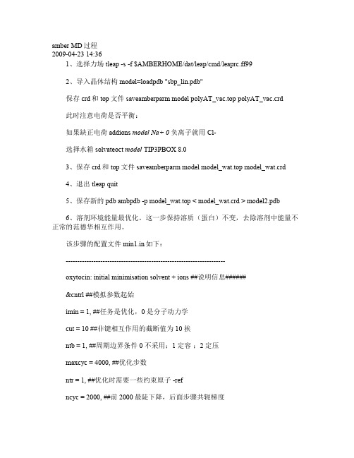
amber MD过程2009-04-2314:361、选择力场tleap-s-f$AMBERHOME/dat/leap/cmd/leaprc.ff992、导入晶体结构model=loadpdb"sbp_lin.pdb"保存crd和top文件saveamberparm model polyAT_vac.top polyAT_vac.crd此时注意电荷是否平衡:如果缺正电荷addions model Na+0负离子就用Cl-选择水箱solvateoct model TIP3PBOX8.03、保存crd和top文件saveamberparm model model_wat.top model_wat.crd4、退出tleap quit5、保存新的pdb ambpdb-p model_wat.top<model_wat.crd>model2.pdb6、溶剂环境能量最优化。
这一步保持溶质(蛋白)不变,去除溶剂中能量不正常的范德华相互作用。
该步骤的配置文件min1.in如下:---------------------------------------------------------------------oxytocin:initial minimisation solvent+ions##说明信息######&cntrl##模拟参数起始imin=1,##任务是优化,0是分子动力学cut=10##非键相互作用的截断值为10挨ntb=1,##周期边界条件0不采用;1定容;2定压maxcyc=4000,##优化步数ntr=1,##优化时需要一些约束原子-refncyc=2000,##前2000最陡下降,后面步骤共轭梯度/Hold the protein fixed##约束说明500.0##作用在肽键上的力kcal/molRES19##限制的残基序号同restrain=’:1-9’ENDEND------------------------------------------------------------------------------任务命令:如果sander-O-i min1.in-p model_wat.top-c model_wat.crd-o min1.out-r min1.rst–ref model_wat.crd&7、对蛋白进行优化,min2.in文件将min1.in中的限制原子修改,限制水的位置。
gromacs 参数

GROMACS 参数GROMACS(Groningen Machine for Chemical Simulations)是一个用于分子动力学模拟的软件包。
它是一个强大且广泛使用的工具,可用于研究分子系统的运动和相互作用。
在使用GROMACS进行模拟之前,需要设置一些参数来定义模拟的条件和系统的性质。
本文将介绍一些常用的GROMACS参数及其含义。
1. 模拟系统参数1.1 动力学集合GROMACS支持多种动力学集合,用于定义系统在模拟过程中的行为。
常用的动力学集合包括:•NVT集合:系统的粒子数(N)、体积(V)和温度(T)保持不变。
•NPT集合:系统的粒子数(N)、压力(P)和温度(T)保持不变。
•NVE集合:系统的粒子数(N)、体积(V)和能量(E)保持不变。
1.2 算法参数GROMACS使用一些算法来模拟分子系统的运动。
以下是一些常用的算法参数:•步长(dt):模拟的时间步长,用于更新粒子的位置和速度。
•非键相互作用截断半径(rlist):用于计算非键相互作用的截断半径。
•范德华相互作用截断半径(rvdw):用于计算范德华相互作用的截断半径。
•电静势相互作用截断半径(rcoulomb):用于计算电静势相互作用的截断半径。
2. 分子参数2.1 力场力场是描述分子间相互作用的数学模型。
GROMACS支持多种力场类型,包括:•GROMOS力场:适用于有机和生物分子的模拟。
•AMBER力场:适用于生物分子的模拟。
•CHARMM力场:适用于生物分子的模拟。
•OPLS力场:适用于有机和生物分子的模拟。
2.2 溶剂模型在模拟中,常常需要考虑溶剂对分子的影响。
GROMACS提供了多种溶剂模型,包括:•SPC水模型:适用于模拟水溶液。
•TIP3P水模型:适用于模拟水溶液。
•TIP4P水模型:适用于模拟水溶液。
2.3 原子参数GROMACS使用原子的质量、电荷和力场参数来描述分子系统。
这些参数通常从力场文件中读取,包括:•原子质量(mass):原子的质量。
分子动力学模拟技术的使用技巧
分子动力学模拟技术的使用技巧简介:分子动力学模拟(Molecular Dynamics Simulation,简称MD)是一种用于模拟分子体系行为的计算方法。
它通过数值计算分子间的相互作用,模拟出分子的运动轨迹和物理性质。
在材料科学、生物医学、化学等领域,MD模拟技术已经成为一种常用的工具,用于深入研究分子系统的动态行为。
本文将介绍一些使用MD模拟技术的技巧和注意事项。
一、系统建模在进行MD模拟之前,我们首先需要建立系统的几何模型和参数设置。
建模过程需要注意以下几点:1. 选择适当的力场:不同的分子体系需要采用适合的力场模型。
一般可以选择常用的力场模型如Amber、CHARMM、OPLS等。
2. 确定原子排布和边界条件:根据实际问题和研究目的,确定分子体系中原子的初始位置和速度,并设置边界条件,如周期边界条件。
3. 添加溶剂模型:对于溶液模拟,需要添加适当的溶剂模型,并考虑其浓度、大小等参数。
二、模拟参数设定在进行MD模拟之前,我们需要设定一些重要的模拟参数,如时间步长、温度、压力等,以确保模拟的准确性和可靠性。
以下是一些常见的参数设定技巧:1. 时间步长选择:较小的时间步长可以提高模拟的准确性,但也会增加计算量。
一般可以通过试验不同的时间步长来选择合适的数值。
2. 温度控制:可以使用恒定温度算法,如Berendsen算法或者Nosé-Hoover算法,来控制模拟系统的温度,并达到平衡状态。
3. 压力控制:在模拟中可以使用恒定压力算法,如Berendsen算法或者Parrinello-Rahman算法来控制模拟系统的压力,并保持平衡状态。
三、模拟过程控制在进行MD模拟过程中,我们需要关注模拟过程的控制和调试。
以下是一些常用的技巧:1. 平衡模拟:在进行有限模拟之前,可以进行一段时间的预处理,用于让体系达到平衡状态。
通常可以通过模拟体系内部能量的变化和物理性质的平衡来判断平衡状态是否达到。
amber实战

第一步:生成小分子模板蛋白质中各氨基酸残基的力参数是预先存在的,但是很多模拟过程会涉及配体分子,这些有机小分子有很高的多样性,他们的力参数和静电信息不可能预存在库文件中,需要根据需要自己计算生成模板。
amber中的antechamber 程序就是生成小分子模板的。
生成模板要进行量子化学计算,这一步可以由antechamber中附带的mopac完成,也可以由gaussian完成,这里介绍用gaussian计算的过程。
建议在计算前用sybyl软件将小分子预先优化,不要用gaussian优化,大基组从头计算进行几何优化花费的计算时间太长。
gaussian计算的输入文件可以用antechamber程序直接生成,生成后去掉其中关于几何优化的参数即可将小分子优化后的结构存储为mol2各式,上传到工作目录,用antechamber程序生成gaussian 输入文件,命令如下:antechamber -i 49.mol2 -fi mol2 -o 49.in -fo gzmat这样可以生成49.in文件,下载到windows环境,运行gaussian计算这个文件,如果发现计算时间过长或者内存不足计算中断,可以修改文件选择小一些的基组。
获得输出文件49.out之后将它上传到工作目录,再用antechamber生成模板,命令如下:antechamber -i 49.out -fi gout -o 49mod.mol2 -fo mol2 -c resp运行之后就会生成一个新的mol2文件,如果用看图软件打开这个文件会发现,原子的颜色很怪异,这是因为mol2的原子名称不是标准的原子名称,看图软件无法识别。
下面一步是检查参数,因为可能会有一些特殊的参数在gaff中不存在需要程序注入,命令如下:parmchk -i 49mod.mol2 -f mol2 -o 49mod这样那些特殊的参数就存在49mod这个文件中了第二步:处理蛋白质文件amber自带的leap程序是处理蛋白质文件的,他可以读入PDB格式的蛋白质文件,根据已有的力场模板为蛋白质赋予键参数和静电参数。
Amber使用笔记B3
Amber使用笔记B3- Case Study: Folding TRP Cage (Advanced analysis and clustering)---Written by PanLu Introduction:1)"Trpcage" ,含有20个氨基酸残基,是可以显示两态折叠性质且在室温下稳定的最小的一个氨基酸;Section 1:创建构型1)建一个线性的多肽链时,Leap工具不会自动识别这个链的两端,因此,我们要明确这个链的N端(在氨基酸前加一个N)和C端(在氨基酸前加一个C);使用命令:肽链名= sequence {氨基酸按顺序排列}2)文献上使用的leaprc.ff99力场在高版本的Amber11中没有,我使用了leaprc.ff99SB这个力场;3)分别保存了一个lib文件(saveoff命令,AmberTools13 Reference Manual P125,save UNITs and PARMSETs using the Object File Format, 这个文件是用来干什么的?)和一个pdb文件(savepdb命令,便于VMD可视化)。
Section 2:创建prmtop和inpcrd文件1)文献中提到使用了FF99力场,但Amber6版本并没有FF99力场,作者实际使用了修改了phi/psi二面角参数的FF99力场;由于这种的修正可能会导致glycine参数化的问题,在Amber9版本中这种修正被删除,而FF99力场也被FF99SB力场替代;2)在生成prmtop文件和inpcrd文件之前,先使用了loadoff命令调用了lib文件,然后使用loadamberparams命令上载了一个替代的二面角参数文件,之后才使用saveamberparm命令保存prmtop和inpcrd文件;3)在我们的工作中,直接使用了FF99SB力场,不考虑这种二面角的修正;Section 3:优化Section 4:heating1) 既然已经在前面做了结构优化,为什么不直接做动力学,而要先做heating ? 2) “MD simulations of 100 ns were performed at 300 K, but all were kineticallytrapped on this time scale, showing strong dependence on initial conditions and failing to converge to similar conformational ensembles. We therefore increased the temperature to 325 K.” 因此,在这个工作中,没有在300K 温度下做MD ,而是将温度升至325K;3) 由于我们的初始结构是人工构建而不是实验的晶体结构,在开始heating 时相比实验结构会不太稳定,所以,在heating 过程中,该工作time step 设置为0.5fs ,而在平衡之后的MD 过程,time step 为2fs ;4) Heating 过程分7步,可以发现从300K~325K 过程,花了较长的时间和步数,为什么?5)6)Tutorial中提供的csh脚本在我们的服务器上并不适合,作业并不能依次提交,因此,我们还是手动的一个作业一个作业地提交;7)使用了一个节点4个cpu并行的计算,大约10个小时可完成一个作业,并行化的使用为:Export DO_PARALLEL=’mpirun –np 4’DO_PARALLEL $AMBERHOME/exe/sander ……Section 5:Production MD1)在做完之前一系列的准备工作之后,可以开始在325K下的long production(?)MD模拟。
amberlite xad-4 中文说明书
注意事项:请勿在这些材料中使用硝酸或其他强氧化剂。
用有机溶剂(如甲醇,乙醇或异丙醇)洗脱可导致这些树脂溶胀。
使用足够的树脂仅填充色谱柱。
当使用树脂溶胀溶剂时,这将允许膨胀的空间。
树脂润湿程序大多数这些材料以湿的形式供应。
但是,在运输和/或储存过程中长时间暴露在空气中可能会导致材料干燥。
除非应用是空气采样,否则材料必须在使用前润湿。
按照此处列出的步骤操作。
1.将干树脂转移到500mL烧杯中。
加入足够的甲醇以覆盖树脂床1-2英寸(2.5-5厘米)。
2.轻轻搅拌树脂一分钟,确保完全混合。
让材料静置15分钟。
3.小心滗出大部分甲醇,并用蒸馏水代替。
搅拌混合物,然后静置5-10分钟。
请遵循以下列准备说明。
柱的制备制备色谱柱时,务必使用完全水合的树脂。
如有必要,按照上述步骤润湿材料,并且在制备或随后使用过程中不要让树脂床干燥。
在树脂床上方约1英寸(2.5厘米)水或溶剂的恒定头部将防止树脂脱水并减少床中的通道。
1.在添加树脂浆料之前,向空柱中加入约1“(2.5cm)的去离子水。
2.将树脂浆料缓慢倒入色谱柱中。
当色谱柱填充时,将多余的水排出色谱柱底部,但不要让液位低于树脂床的顶部。
添加足够的树脂,仅填充半柱。
当使用树脂溶胀溶剂时,这将允许膨胀的空间。
反冲洗这个过程去除了气泡,对树脂颗粒进行了分类(允许它们根据尺寸分层,在柱顶部形成最小的颗粒),并且排出新的树脂细粒床(小颗粒)。
大约30分钟的反洗通常足以在新柱中准备床。
对于使用中的色谱柱,反洗可去除床中收集的碎屑。
通常,在洗涤吸附物之前,在吸附物吸附到树脂上之后对床进行反洗。
1.在水柱底部安装水管。
2.引入缓慢向上流动的去离子水。
小心地增加流量,直到整个树脂床悬浮。
3.保持水流直至所有气泡脱落。
树脂细粉将从柱顶部排出。
4.停止水流,让树脂沉淀。
5.将水位调节到树脂床顶部上方1英寸(2.5厘米)或更高的位置。
确定床体积填充柱后,反洗并使其沉降,并调整液位,确定柱中树脂的体积:圆柱体积= ∏x (1/2 inside diameter)2 x length of the bed该值“床体积”有助于正确操作色谱柱。
amber力场计算公式
amber力场计算公式Amber力场是一种经典力场,用于计算和描述分子体系中的相互作用和能量。
它基于分子力学的原理和假设,通过引入势能函数来描述分子之间的相互作用。
Amber力场的计算公式可以分为以下几个部分:键能、角能、二面角能、范德华能、电位能以及其他项的贡献。
1. 键能(Bond Energy):用于描述和计算化学键的形成和断裂过程。
键能的计算公式通常采用调和近似,即将键能视为一个弹簧,键的能量可以表示为:E_bond = 1/2 * k_bond * (r - r_0)^2其中,E_bond是键的能量,k_bond是键的弹性常数,r是键的实际长度,r_0是键的平衡长度。
2. 角能(Angle Energy):用于描述和计算相邻键之间的角度。
角能的计算公式通常也采用调和近似,即将角能视为一个弹簧,角的能量可以表示为:E_angle = 1/2 * k_angle * (theta - theta_0)^2其中,E_angle是角的能量,k_angle是角的弹性常数,theta是角的实际大小,theta_0是角的平衡大小。
3. 二面角能(Dihedral Energy):用于描述和计算分子中的二面角(torsion)的变化。
二面角能的计算公式通常由多个正弦和余弦函数组成。
这些函数的系数取决于分子的几何结构和化学键的性质。
4. 范德华能(Van der Waals Energy):用于描述和计算分子中非键的相互作用。
范德华能的计算公式通常采用Lennard-Jones势能函数,可以表示为:E_vdw = 4 * epsilon * ((sigma/r)^12 - (sigma/r)^6)其中,E_vdw是范德华能,epsilon是能量参数,sigma是长度参数,r是两个分子之间的距离。
5. 电位能(Electrostatic Energy):用于描述和计算带电粒子之间的相互作用。
电位能的计算公式通常采用库仑势能函数,可以表示为:E_elec = k_e * q1 * q2 / r其中,E_elec是电位能,k_e是库仑常数,q1和q2是带电粒子的电荷,r是两个分子之间的距离。
amber 分子动力学计算
amber 分子动力学计算
Amber 是一种广泛使用的分子动力学模拟软件,用于研究生物分子的结构、动力学和热力学性质。
以下是 Amber 分子动力学计算的一般步骤:
1. 准备初始结构:使用分子建模软件(如 Maestro、PyMol 等)构建所需研究的分子体系的初始结构。
2. 设定力场参数:选择适合的力场(如 Amber99、 Amber14 等)并设置相应的参数,如键长、键角、二面角等。
3. 定义模拟盒子:根据分子体系的大小和形状,定义一个合适的模拟盒子,以包含分子。
4. 填充溶剂:在模拟盒子中加入足够数量的溶剂分子,以模拟所需的溶液环境。
5. 能量最小化:对初始结构进行能量最小化,以消除体系中的不合理结构和高能量构型。
6. 设定模拟参数:设置模拟的时间步长、温度、压力等参数。
7. 执行分子动力学模拟:根据设定的参数,运行分子动力学模拟,记录体系在不同时间点的结构和能量信息。
8. 分析结果:对模拟结果进行分析,如计算均方根偏差(RMSD)、研究分子间相互作用等。
9. 可视化:使用可视化软件(如 VMD、PyMol 等)将模拟结果以图形化的方式展示出来。
需要注意的是,Amber 分子动力学计算是一个复杂的过程,需要一定的计算资源和专业知识。
在进行计算之前,建议对相关理论和方法有一定的了解,并根据具体研究问题选择合适的计算策略。
- 1、下载文档前请自行甄别文档内容的完整性,平台不提供额外的编辑、内容补充、找答案等附加服务。
- 2、"仅部分预览"的文档,不可在线预览部分如存在完整性等问题,可反馈申请退款(可完整预览的文档不适用该条件!)。
- 3、如文档侵犯您的权益,请联系客服反馈,我们会尽快为您处理(人工客服工作时间:9:00-18:30)。
amber动力学常用参数说明个人日记2009-05-08 19:32:18 阅读130 评论1 字号:大中小订阅IMIN Flag to run minimization=0 No minimization (only do molecular dynamics;default)= 1 Perform minimization (and no molecular dynamics)=5 Read in a trajectory for analysis.NTX Option to read the initial coordinates, velocities and box size from the "inpcrd" file. The options 1-2 must be used when one is starting from minimized or model-built coordinates. If an MD restrt file is used as inpcrd, thenoptions 4-7 may be used.= 1 X is read formatted with no initial velocity information (default)= 2 X is read unformatted with no initial velocity information= 4 X and V are read unformatted.= 5 X and V are read formatted; box information will be read if ntb>0. The velocity information will only be used if irest=1.= 6 X, V and BOX(1..3) are read unformatted; in other respects, this is the same as option "5".=7 Same as option "5"; only included for backward compatibility with earlier versions of Amber. IREST Flag to restart the run.= 0 Noeffect (default)= 1 restart calculation. Requires velocities in coordinate input file, so you also may need to reset NTX if restarting MD.NTRX Format of the Cartesian coordinates for restraint from file "refc". Note: the program expects file "refc" to contain coordinates for all the atoms in the system. A subset for the actual restraints is selected by restraintmask in the controlnamelist.= 0 Unformatted (binary) form= 1 Formatted (ascii, default) formNTPR Every NTPR steps energy information will be printed in human-readable form to files "mdout" and "mdinfo". "mdinfo" is closed and reopened each time, so it always contains the most recent energy and temperature. Default 50.NTWR Every NTWR steps during dynamics, the "restrt" file will be written, ensuring that recovery from a crash will not be so painful. In any case, restrt is written ev ery NSTLIM steps for both dynamics and minimization calculations. If NTWR<0, a unique copy of the file, restrt_nstep, is written every abs(NTWR) steps. This option is useful if for example one wants to run free energy perturbations from multiple starting points or save a series of restrt files for minimization. Default 500.NTF Force evaluation. Note: If SHAKE is used (see NTC), it is not necessary to calculate forces for the constrained bonds.= 1 complete interaction is calculated (default)= 2 bond interactions involving H-atoms omitted (use with NTC=2)= 3 all the bond interactions are omitted (use with NTC=3)= 4 angle involving H-atoms and all bonds are omitted= 5 all bond and angle interactions are omitted= 6 dihedrals involving H-atoms and all bonds and all angle interactions are omitted= 7 all bond, angle and dihedral interactions are omitted= 8 all bond, angle, dihedral and non-bonded interactions are omittedNTB Periodic boundary. If NTB .EQ. 0 then a boundary is NOT applied regardless of any boundary condition information in the topology file. The value of NTB specifies whether constant volume or constant pressure dynamics will be used. Options for constant pressure are described in a separate section below.= 0 no periodicity is applied and PME is off= 1 constant volume (default)= 2 constant pressureIf NTB .NE. 0, there must be a periodic boundary in the topology file. Constant pressure is not used in minimization (IMIN=1, above). For a periodic system, constant pressure is the only way to equilibrate densityif the starting state is not correct. For example, the solvent packing scheme used in LEaP can result in a net void when solvent molecules are subtracted which can aggregate into "vacuum bubbles" in a constant volume run. Another potential problem are small gaps at the edges of the box. The upshot is that almost every system needs to be equilibrated at constant pressure (ntb=2, ntp>0) to get to a proper density. But be sure to equilibrate first (at constant volume) to something close to the final temperature, before turning on constant pressure.CUT This is used to specify the nonbonded cutoff, in Angstroms. For PME, the cutoff is used to limit direct space sum, and the default value of 8.0is usually a good value. When igb>0, the cutoff is used to truncate nonbonded pairs (on an atom-by-atom basis); here a larger value than the default is generally required. A separate parameter (RGBMAX) controls the maximum distance between atom pairs that will be considered in carrying out the pairwise summation involved in calculating the effective Born radii, see the generalized Born section below.IBELLY Flag for belly type dynamics.= 0 No belly run (default).= 1 Belly run. A subset of the atoms in the system will be allowed to move, and the coordinates of the rest will be frozen. The moving atoms are specified bellymask. This option is not available when igb>0. Note also that this option does not provide any significant speed advantage, and is maintained primarily for backwards compatibilitywith older version of Amber. Most applications should use the ntr variable instead to restrain parts of the system to stay close to some initial configuration.NTR Flag for restraining specified atoms in Cartesian space using a harmonic potential. The restrained atoms are determined by the restraintmask string. The force constant is given by restraint_wt. The coordinates are read in "restrt" format from the "refc" file (see NTRX, above). = 0 No position restraints (default) = 1 MD with restraint of specified atomsMAXCYC The maximum number of cycles of minimization. Default 1.NCYC If NTMIN is 1 then the method of minimization will be switched from steepest descent to conjugate gradient after NCYC cycles. Default 10.NSTLIM Number of MD-steps to be performed. Default 1.TEMP0Reference temperature at which the system is to be kept, if ntt > 0. Note that for temperatures above 300K, the step size should be reduced since increased distance traveled between evaluations can lead to SHAKE and other problems. Default 300.TEMPI Initial temperature. For the initial dynamics run, (NTX .lt. 3) the velocities are assignedfrom a Maxwellian distribution at TEMPI K. If TEMPI = 0.0, the velocities will be calculated from the forces instead. TEMPI has no effect if NTX .gt. 3. Default 0.0.NTT Switch for temperature scaling. Note that setting ntt=0 corresponds to the microcanonical (NVE) ensemble (which should approach the canonical one for large numbers of degrees of freedom). Some aspects of the "weak-coupling ensemble" (ntt=1) have been examined, and roughly interpolate between the microcanonical and canonical ensembles [63]. The ntt=2 and 3 options correspond to the canonical (constant T) ensemble. The ntt=4 option is included for historical reasons, but does not correspond to any of the traditionalensembles.= 0 Constant total energy classical dynamics (assuming that ntb<2, as should probably always be the case when ntt=0).= 1 Constant temperature, using the weak-coupling algorithm [64]. A single scaling factor is used for all atoms. Note that this algorithm just ensures that the total kinetic energy is appropriate for the desired temperature; it does nothing to ensure that the temperature is even over all parts of the molecule. Atomic collisions should serve to ensure an even temperature distribution, but this is not guaranteed, and can be a particular problem for generalized Born simulations, where there are no collisions with solvent. Other temperature coupling options (especially ntt=3) should probably be used for generalized Born simulations.= 2 Andersen temperature coupling scheme [65], in which imaginary "collisions" randomize the velocities to a distribution corresponding to temp0 every vrand steps. Note that in between these "massive collisions",the dynamics is Newtonian. Hence, time correlation functions (etc.) can be computed in these sections, and the results averaged over an initial canonical distribution. Note also that too high a collision rate (too small a value of vrand) will slow down the speed at which the molecules explore configuration space, whereas too low a rate means that the canonical distribution of energies will be sampled slowly. A discussion of this rate is given by Andersen [66].= 3 Use Langevin dynamics with the collision frequency γ given by gamma_ln, discussed below. Note that when γ has its default value of zero, this is the same as setting ntt = 0.GAMMA_LN The collision frequency γ , in ps-1, when ntt = 3. A simple Leapfrog integrator is used to propagate the dynamics, with the kinetic energy adjusted to be correct for the harmonic oscillator case [67,68]. Note that it is not necessary that γ approximate the physical collision frequency. In fact, it is often advantageous, in terms of sampling or stability of integration, to use much smaller values. Default is 0NTP Flag for constant pressure dynamics. This option should be set to 1 or 2 when Constant Pressure periodic boundary conditions are used (NTB = 2).= 0 Used with NTB not = 2 (default); no pressure scaling= 1 md with isotropic position scaling= 2 md with anisotropic (x-,y-,z-) pressure scaling: this should only be used with orthogonal boxes (i.e. with all angles set to 90). Anisotropic scaling is primarily intended for non-isotropic systems, such as membrane simulations, where the surface tensions are different in different directions; it is generally not appropriate for solutes dissolved in water.NTC Flag for SHAKE to perform bond length constraints [70]. (See also NTF in the Potential function section. In particular, typically NTF = NTC.) The SHAKE option should be used for most MD calculations. The size of the MDtimestep is determined by the fastest motions in the system. SHAKE removes the bond stretching freedom, which is the fastest motion, and consequently allows a larger timestep to be used. For water models, a special "three-point" algorithm is used [71]. Consequently, to employ TIP3P set NTF = NTC = 2. Since SHAKE is an algorithm based on dynamics, the minimizer is not aware of what SHAKE is doing; for this reason, minimizations generally should be carried out without SHAKE. One exception is short minimizations whose purpose is to remove bad contacts before dynamics can begin.= 1 SHAKE is not performed (default)= 2 bonds involving hydrogen are constrained= 3 all bonds are constrained (not available for parallel runs in sander)。