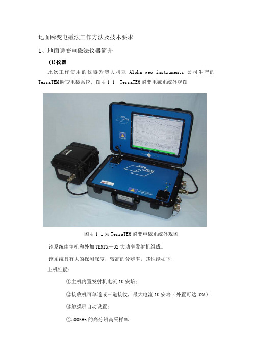
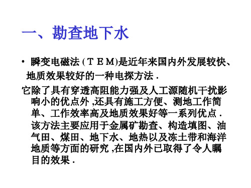
国外瞬变电磁法共37页文档
地面瞬变电磁法技术要求 Microsoft Word 文档
d)点距和观测精度要求应能够保证清晰完整的反映异常细节;
野外工作方法及技术要求
地面瞬变电磁法测量工作方法及技术要求参照中华人民共和国地质矿产行业标准DZ/T0187—1997《地面瞬变电磁法技术规程》来执行。
野外工作前对仪器进行了检查和调试,仪器正常方可投入生产。仪器设备严格按照操作规程执行。
2、瞬变电磁野外工作方法及技术要求
参数设置
根据工作区实际地质情况和任务要求,重叠回线Tx、Rx边长为 300 m×300m,面积为90000m2,采用主机供电测量,电压为24V,回路电阻为8Ω,电流为3A ,延迟0.025~6.9ms,采样间隔时间为0.1ms,采样数为74。叠加次数的选取视各观测点的干扰电平而定,一般为512~2048次。
接收站布置在远离强干扰源以及金属干扰物的地方。
不得在上万伏高压线下布设发送站及接收站,有必要时允许弃点。
发送站、接收站应配备测伞。阴雨湿度很大及雷雨天气不宜开展工作。
敷设线框时,剩余导线将其呈“S”型铺于地面。布线时导线在方向线上摆动幅度不得大于回线边长的5%。并适时检查导线的绝缘性。
导线连接处接触良好,不得漏电。导线的绝缘电阻大于2M·Ω。
(2) 装置类型
图4-1-2重叠回线装置示意图
本次探测采用重叠回线装置,即发射线框和接收线框规格相同。该装置与目的物耦合最紧,发射线圈逐测点移动,不会有激发盲区,发射磁矩和接收磁矩较大,异常形态简单,横向分辨率高,易于分析。4-1-2为重叠回线装置示意图。RX接收回线观测参数为用发射电流归一的感应电动势。
当导线通过水田、池塘、河沟时,应予架空,防止漏电;当导线横过公路时,应架空或埋于地下以防绊断压坏。导线架空处拉紧,防止随风摆动。
瞬变电磁法,国外高清资料
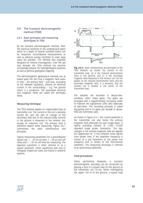
4.4 The transient electromagnetic method (TEM)4.4The transient electromagnetic method (TEM)4.4.1 Basic principles and measuring techniques in TEMBy the transient electromagnetic method, TEM, the electrical resistivity of the underground layers down to a depth of several hundred meters can be measured. Groundbased measurements as well as airborne surveys (SkyTEM) to cover large areas are possible. The method was originally designed for mineral investigations. Over the last two decades the TEM method has become increasingly popular for hydrogeological purposes as well as general geological mapping. The electromagnetic geophysical methods are all based upon the fact that a magnetic field varies in time – the primary field – and thus, according to the Maxwell equations, induces an electrical current in the surroundings – e.g. the ground which is a conductor. The associated electrical and magnetic fields are called the secondary fields.Fig. 4.4.1: Basic nomenclature and principles of the TEM method. (a) Shows the current in the transmitter loop. (b) Is the induced electromotive force in the ground, and (c) is the secondary magnetic field measured in the receiver coil. For the graphs of the induced electromotive force and the secondary magnetic field, it is assumed, that the receiver coil is located in the centre of the transmitter loop.Measuring techniqueThe TEM method applies an ungrounded loop as transmitter coil. The current in the coil is abruptly turned off, and the rate of change of the secondary field due to the induced eddy currents in the ground is measured in the receiver coil, usually an induction coil. The primary field is therefore absent while measuring. Figure 4.4.1 summarizes the basic nomenclature and principles. Typical measuring parameters for a groundbased system are: 1 – 20 ms on-time, 1 – 30 μs turn-off ramp and 1 – 20 ms off-time for measuring. The depicted waveform is often referred to as a square waveform. Other waveforms with sine or triangular shapes are used, but mainly in airborne systems.The datasets are recorded in decay-timewindows, often called gates. The gates are arranged with a logarithmically increasing width to improve the signal/noise (S/N) ratio especially at late-times. This recording principle is called log-gating and 8–10 gates per decade in decaytime are commonly used. As shown in Figure 4.4.1, the current polarities in the transmitter coil and hence the primary magnetic field alternates for each single pulse. A typical sounding consists of 1,000 – 10,000 repeated single pulses (transients). The sign changes in the primary magnetic field are applied for suppression of: 1) the coherent noise signals from power lines, if the repetition frequency is chosen as a sub harmonics of the power line frequency and 2) offsets of the instrumental amplifiers. This measuring technique is referred to as synchronous detection.Field proceduresWhen performing fieldwork, a transient electromagnetic sounding can be conducted by placing a wire in a square loop on the ground as the transmitter coil, Tx-coil. When investigating the upper 150 m of the ground, a square loop65KURT I. SØRENSEN, ANDERS VEST CHRISTIANSEN & ESBEN AUKENwith an area of 40 x 40 m is commonly used. The receiver coil, Rx-coil, with a diameter of approximately 1 m is placed in the centre of the transmitter coil.2The TEM principleThe measurements are carried out by ejecting a current in the Tx-loop. This results in a static primary magnetic field. The current is turned off abruptly and the related change in the primary magnetic field induces an electromotive force in the conducting surroundings. In the ground, this electrical field will result in a current which again will result in a magnetic field, the secondary field. Just after the transmitter is switched off, the secondary magnetic field from the current in the ground will be equivalent to the primary magnetic field (which is no longer there). As time passes by, the resistance in the ground will still weaken the current (converted to heat), and the current density maximum will eventually move outwards and downwards, leaving the current density still weaker. The decaying secondary magnetic field is vertical in the middle of the Tx-loop (at least if the ground consists in plane and parallel layers). Hereby an electromotive force is induced in the Rx-coil. This signal is measured as a function of time. Just after the current in the Tx-loop is turned off, the current in the ground will be close to the surface, and the measured signal reflects primarily the resistivity of the top layers. At later decay-times the current has diffused deeper into the ground, and the measured signal then contains information about the resistivity of the deeper layers. Measuring the current in the Rxcoil will therefore give information about the resistivity as a function of depth. The configurations shown in Figure 4.4.2 have the receiver coil placed in the centre of the Tx-coil and is called a central loop or an in-loop configuration. The receiver coil can be placed outside the Tx-loop which results in an offsetloop configuration.Fig. 4.4.2: Field setup of a TEM system: a) Shows a central loop configuration, b) an offset-loop configuration. Rx denotes the receiver, Tx the transmitter, l the side length of the loop and h the offset between Tx-coil and Rx-coil centres.4.4.2 Data curvesThe decaying secondary magnetic field is referred to as b or the step response. However, because an induction coil is used for measurements of the magnetic field, the actual measurement is that of db/dt, the impulse response (the induced electromotive force is proportional to the time derivative of the magnetic flux passing the coil). The impulse response, db/dt is plotted in Figure 4.4.3 for a variety of halfspace resistivities.Fig. 4.4.3: In a) the impulse responses (db/dt) for a homogeneous halfspace with varying resistivities are presented (black lines). The same curves converted to ρa are shown in b). The grey line is the response of a two-layer earth with 100 Ωm in layer 1 and 10 Ωm in layer 2. Layer 1 is 40 m thick.664.4 The transient electromagnetic method (TEM)Figure 4.4.3 indicates power function dependence at late-times. At late-times, the impulse response can be written as∂b z - Iσ 3 2μ 0 a 2 -5 2 ≈ t ∂t 20π 1 252(4.4.1)As seen db/dt has a decay development -5/2 proportional to t . Observation of the decaying magnetic field in Figure 4.4.3 is not very informative and the same applies for actually measured sounding curves. A plot of apparent resistivity, ρa, is more illustrative. It is derived from the late-time approximation of the impulse responseρa = ( Ia2 μ5 3 )1 / 2 0 3 t -5 3 20 ∂bz ∂t π1(4.4.2)The response curves plotted in Figure 4.4.3a are shown as ρa-converted curves in Figure 4.4.3b. The ρa-converted curves can be used as a data quality tool and as first estimate of the resistivity levels of the underground structure.Fig. 4.4.4: TEM sounding curves stacked with 50 transients (grey) and 5,000 transients (black).4.4.3 Background noiseA geophysical datum always consists of two numbers – the measurement itself and the uncertainty of the measurement. One single transient is affected significantly by the electromagnetic background noise. By repeating and stacking the measurement the background noise is decreased and the signal enhanced. Generally, a TEM sounding may consists of 1,000 to 10,000 single transients. Figure 4.4.4 shows stacks of 50 single transients and a stack of 5,000 single transients. It is obvious that a sounding with 5,000 stacked transients has a much better signal-to-noise ratio, S/N ratio, compared to the stack with 50 transients.The electromagnetic background noise originates from various sources. Most sources, such as lightnings, are very distant. The fields from these sources travel around the globe in the wave guide cavity between the surface of the Earth and the ionosphere. This noise has a random character, and it is more powerful during the day than during the night and stronger during summer compared to winter. Background noise also originates from the power supply and the related man-made electrical installations. There are partly the 50 or 60 Hz signals and its harmonics, which have a deterministic character, partly the transient fields, which are of a random character and related to current changes in the power lines, when various installations are turned on or off. The deterministic part of the background noise from the power supply is removed by synchronous detection techniques, as mentioned before.67KURT I. SØRENSEN, ANDERS VEST CHRISTIANSEN & ESBEN AUKENWith well-designed equipment the noise contribution from the electronics in the instrument itself is negligible compared to the noise contributions described above. It can be shown that using the log-gating technique, random noise contributions are decreasing -1/2 proportional to t . It is evident that the signal level of measurements at early-times in most cases is many times larger than the noise level. This implies that the S/N ratio is high, and the uncertainty of the measurements is low at early-times. At later decay-times the decay signal is proportional to -5/2 t . As the random noise level is proportional to -1/2 t it implies that the transition from a good S/N ratio to a poor S/N ratio happens quite suddenly. There are two ways to obtain datasets of a satisfactory S/N ratio at later decay-times, i.e. information from larger depths: 1) reduce the noise by increasing stack size or 2) increase the transmitted moment. Stacking reduces the noise proportional to N where N is the number of measurements in the stack. The effect of increasing the moment is shown in Figure 4.4.5 with the black dotted line. The line indicates the level of a sounding at the same location with a ten times larger moment and it is clear that the S/N ratio is much higher at later decay-times increased by a factor of ten.Fig. 4.4.5: TEM sounding and noise measurements. The grey curves are noise measurements with the -1/2 t trend plotted with the thick dashed grey line. Error bars are 5%. The earth response is the black curves. The black dotted line indicates the approximate level of a sounding with a 10 times higher transmitter moment.4.4.4 Penetration depthIn relation to TEM soundings it is difficult, as for all other geophysical methods, to speak quantitatively and unambiguously about the penetration depth. In the following we will state some rules of thumb. The depth down to which the current system has diffused is called the diffusion depth. This depth, zd, is defined byThis is an exact equation for plane fields only. For circular or quadratic loop sources the diffusion depth is about 1.8 times smaller than estimated by Equation 4.4.3. As seen in the Figure 4.4.3, the signal decreases -5/2 in a homogenous halfspace by t , and when the signal passes the level of the background noise, we can no longer use the measurements. Thus, the level of the background noise sets the limits for how late we can use our measurements. By using the expression given for dbz/dt for latetimes we find a relationship between the noise signal, Vnoise, and the latest decay-time at which we can make measurements:zd =2t ≈ .26 × ρt [m] , 1 μσρ [Ωm], t [μs](4.4.3)684.4 The transient electromagnetic method (TEM)tL = μ (M )2 / 5 20 Vnoiseσ ( )3 / 5 π(4.4.4)When tL is equivalent with the diffusion time tdzd = ( 2 1 / 10 ) 25 π 3 ( M 1/ 5 M 1/ 5 ) = 0.551 ( ) σVnoise σVnoisedataset within the estimated uncertainties are called equivalent models. Sometimes equivalences can be very pronounced in the sense that very different models give rise to almost identical responses. Equivalence appears in relation to thin good conductors embedded in resistive surrounding and vice versa. In these cases the resolution of the thin layers may be poor resolved.(4.4.5)From these expressions it is seen that the maximal diffusion depth, which is a measure for the penetration depth, is proportional to the fifth root of the ratio between the moment of the current loop and the product of the conductivity and the noise level. The only way to increase the penetration depth is to increase the moment of the transmitter or decrease the effective noise level, being the noise level after stacking and gating. The background noise is a relatively unchangeable size, but the way in which we gather and process our datasets, by stacking many measurements, reduces the effective noise. To double the penetration depth, the effective noise has to be reduced – or – the moment of the transmitter has to be increased by a factor 32.4.4.6 Coupling to man-made installationsDistortion of datasets due to coupling to manmade electrical installations is not noise in the same sense as the random electromagnetic background noise described in the noise section. Coupling noise is a distortion and relates to induced currents in all man-made electrical conductors. The distortion has a deterministic character, arising at the same delay time for all decays and will therefore be summed in the stacking process. Coupling distortion in datasets cannot be accurately removed to provide a reliable interpretation; therefore soundings located close to man-made installations such as pipelines, cables, power lines, rails, auto guards and metal fences cannot be interpreted, and the dataset should be culled. The safe distance, defined as the minimum distance where undistorted datasets can be measured, is counted as the distance between any point on the transmitter-receiver setup and the man-made conductor. The safe distance to any man-made conductor is at least 100 m over an earth with an overall resistivity of 40 – 60 Ωm. The safe distance increases with the resistivity.4.4.5 Resolution and equivalenceThe induced eddy currents are predominantly flowing in the good conducting formations. Therefore the resistivity and the layer boundaries of good conductors are very often well resolved. The eddy currents decay fast in high resistive layers and only weak measurable signals are produced. Hence in the presence of good conductors these signals often are neglectable and the resistivity level of high resistive formations is poorly resolved. In contrary, the layer boundaries may be resolved as these will coincidence with the boundaries of good conductors. The “geometry” of the high resistive formations may therefore be resolved. As mentioned before a geophysical measurement is described by its value and the uncertainty estimate on this value. Models that produce responses which compare to the measured4.4.7 Modelling and interpretation Data acquisitionAs mentioned in the introduction, a main issue in applying the TEM method for hydrogeological studies is the demand for accurate and undisturbed datasets with high spatial density. Insufficient data quality makes it impossible to obtain a reliable geophysical model for use in a hydrogeological context.69KURT I. SØRENSEN, ANDERS VEST CHRISTIANSEN & ESBEN AUKENAn important element of the data quality is the precise knowledge of the parameters of the applied instrument. To obtain datasets of sufficient quality, the following instrumental parameters must be known and modelled in the data modelling algorithm:■■The transmitted waveform characteristics, including the exact appearance of the current turn-off and turn-on ramps and the timing between the transmitter and the receiver actions. Timing parameters must be known to an accuracy of 100 – 200 nanoseconds, because of their severe impact on early-time data. The receiver transfer function, which is modelled by one or more low-pass filters, often has a strong influence on early-time data. Low-pass filters are implemented in the receiver system to stabilize the amplifiers and to suppress the noise from long-wave radio transmitters. The geometry of the transmitter-receiver configuration must be accurate, especially for the offset-loop configuration. Central-loop datasets are relatively insensitive to deviations in geometry as long as the transmitter area is unchanged.■Measuring in the central-loop configuration with a small transmitter coil and high output current may saturate the receiver amplifiers due to high voltages arising from the turn-off of the primary field. After saturation, amplifiers will produce distorted signals for several milliseconds. Furthermore, currents of the order of nanoamperes will leak in the transmitter coil after the current is turned off, adding to the earth's response and thereby to the distortion of the datasets. Both effects become negligible because of geometry when using either a small output current with a large transmitter loop or a large offset between the transmitter and the receiver coils. Thus high-output current datasets using a small transmitter coil must be measured in the offset-loop configuration, while low current datasets can be measured in the central-loop configuration. The induced polarization (IP) effect is present in datasets measured in some sedimentary environments. The IP effect is most pronounced in datasets from the central-loop configuration, but moves to later decay-times when increasing the transmitter coil size. In offset configurations the IP effect is less pronounced and moves to later decay-times as the offset between the transmitter and the receiver coil is increased. At early times, measurements using the offset configuration are extremely sensitive to small variations in the resistivity in the near surface. Extensive 3D modelling of such variations shows a pronounced influence on the measured datasets as the current system passes beneath the receiver coil. In many cases these datasets are not interpretable with a 1D model, even if the section is predominantly 1D. At later times, after the current system has passed, the distorting influence has decayed. Datasets from the central-loop configuration are much less affected by near-surface resistivity variations. Datasets from the offset configuration are sensitive to small deviations in the array geometry. As an example assuming a 60 Ωm half-space model, a 30% error in the decay signal is apparent near the sign change if the receiver coil is located 71 m instead of 70 m■■Measuring datasets with a high spatial density serves two purposes: 1) the resolution of geological structures is improved and 2) distorted datasets caused by instrument malfunction and transmitter-induced coupling to man-made conductors can be revealed and eliminated. The latter is by far the most important.■Configurations, advantages and drawbacksGround-based TEM systems using a high transmitter moment normally utilize a transmitter loop of 40 – 100 m. The advantages of a large loop are that measurements can be carried out at the centre of the loop, and that the magnetic moment is large. The drawbacks are the low field efficiency and the higher possibility of coupling with man-made installations. A small transmitter coil with a high current is very field efficient, but four issues must be tackled in the configuration design:■704.4 The transient electromagnetic method (TEM)from the transmitter. In a routine field situation, it is next to impossible to work with such accuracy. After the sign change, datasets from the offset configuration is essentially equivalent to that of a central-loop configuration. A compromise is to use a high-power system with small transmitter loop, where early-time data are measured in the central loop configuration with a small current of 1 – 3 A. Late-time data are, in turn, measured in the offset configuration with maximum output current. In this way the four issues are addressed, and the field productivity can still be kept high.number of key issues need to be addressed to achieve this high data quality. The issues are mainly related to calibration, altitude and the flight speed.CalibrationIn the context of requiring high data quality, the calibration of the transmitter/receiver system plays a central role. When airborne systems operate in the frequency domain, the strong primary field has to be compensated in order to be able to measure the Earth response. Because of drift in the system the compensation changes in time, and its value has to be determined successively during the survey by high-altitude measurements. Furthermore, it is necessary to perform measurements along tie lines perpendicular to the flight lines and by postprocessing to provide concordance between adjacent lines. This process is called levelling, and because of this a frequency domain system is said to be relatively calibrated. When airborne systems are operating in the time domain, it is possible to reduce the interaction between the transmitter and the receiver system to a level, at which the distortion of the measured off-time signals is negligible. In this case, a calibration of the instrumentation can be performed in the laboratory and/or at a testsite before carrying out the surveys. Neither high altitude measurements nor performing tie lines for levelling are then necessary during the survey. Such a system is said to be absolute calibrated. The SkyTEM system has these capacities. The relatively calibrated systems will have a lower S/N ratio and lower data accuracy because of the drift and the levelling of datasets compared to that of absolutely calibrated systems.The 1D modelTo this day it is not possible to invert TEM datasets in more than one dimension on a routine basis. 3D inversion codes have been developed lately, but they are still computationally very demanding, and require densely measured datasets in at least two dimensions. Therefore, it is inevitable that geological noise, i.e. insufficient model presentation of the actual structure, is present when describing a 3D structure by a 1D model. The distribution of 2D and 3D structures decides the amount of geological noise.4.4.8 Airborne TEMBelow we will present an overview of the requirements to airborne EM systems, especially TEM, and discuss the specific topics where the airborne and the ground based techniques differ. We will focus on the relatively new helicopter system, SkyTEM, as it provides the sufficient accuracy necessary for groundwater investigations. Hence the following comment on the main issues for airborne TEM is related to the application of the SkyTEM method.AltitudeFor all EM airborne systems the Earth response decreases with increasing altitude. The random noise contribution from natural and man-made sources show no significant decrease within the operating altitude range compared toSpecial considerations for airborne electromagnetic measurementsIn groundwater exploration, high quality data are required as the decisive data changes can be as low as 10 – 15 %. When operating airborne a71KURT I. SØRENSEN, ANDERS VEST CHRISTIANSEN & ESBEN AUKENground based measurements. Therefore, a higher operating altitude implies a lower S/N ratio at late-times, where the noise becomes predominant, and results in a poorer resolution of the deeper part of the Earth. The resolution of the near-surface layers decreases with increasing altitude because the induced eddy current system at early-times becomes larger and more spatial averaged. In general, increasing altitude means a lower resolution of upper layers. Another implication of the decaying Earth response with altitudes is increased distortions of the Earth response due to coupling to man-made installations. As mentioned before, a safety distance to installations of at least 100 m, depending on the subsurface structures, has to be maintained in order to avoid distorted datasets. Application of airborne electromagnetic measurements introduces larger safety distances to installations compared to ground based equipment, because Earth responses decreases with increasing altitude, whereas coupling responses in the operation altitudes maintain their signal level. The larger the operating altitude is the larger are the safety distances.The lateral movement while achieving the required stack size increases with velocity which implies a decrease in the lateral resolution. Hence, a higher vertical resolution inevitably means a decreased lateral resolution if the fight speed is unchanged. On the contrary, the same lateral resolution at a higher velocity results in a decrease of the S/N ratio and hence the vertical resolution.Data quality and post-processingAirborne electromagnetic surveys are very cost effective. As the data acquisition is extremely fast, and large amounts of datasets are collected over a short period of time, the data quality control has to be automatic. As discussed before, the application of an absolutely calibrated TEM system, as the SkyTEM system, implies that no high-altitude measurements have to be carried out during the survey and subsequently used for compensating the datasets for the effects from transmitterreceiver interactions. Nor is it necessary to perform levelling of the datasets. In order to maintain the high data quality demanded for groundwater surveys, the geometrical setup of the equipment has to be well determined at all times, as well as the transmitted current waveform. The geometrical setup is determined by the altitude and the inclination of the transmitter and receiver coils. Furthermore, it is essential that the calibration and the functionality of the instruments are well documented, and that all setup parameters are saved for the subsequent interpretation. The post-processing of the measured datasets relates to two tasks. The first task is to process the altitude, inclination and position data in order to remove outliers and to provide continuity. Especially the altitude data need processing as they are, in many cases, affected by the vegetation on the surface. If the altimeter reflections from vegetation are not identified and corrected, errors will be introduced in the interpreted models. Figure 4.4.6 shows a section of altimeter data from the SkyTEM system. The dots are reflections as picked up by one of the laser altimeters mounted on the transmitterFlight speedAn important tool for increasing the S/N ratio in electromagnetic measurements is to perform stacking of the measurements. In TEM measurements the background noise is reduced by stacking the transients. To achieve a required S/N ratio, a certain number of transients are necessary in the stack. When the system is moving while measuring, a trade-off exists between the lateral and the vertical resolution of the Earth parameters because a flight velocity related time interval is needed to collect the transients for the required stack size. The vertical resolution is related to the S/N ratio determined by the stack size. A certain stack size corresponds to a defined acquisition time interval.724.4 The transient electromagnetic method (TEM)frame. The solid line is the processed altimeter data. The effects of the erroneous reflections obtained over the forest are removed in the processed altitude curve. Data from the processed altimeter data are used in the interpretation of the datasets.Fig. 4.4.6: Processing of altitude data. Dots are the actual reflections picked up by a laser altimeter. The solid line is the processed height data. Over the forest a large number of reflections come from the tree-tops.The measured inclination of the frame is used both to correct the altitudes and the datasets. Altitudes are measured assuming that the laser beam is normal to the ground surface. When the laser tilts, the normal altitude has to be calculated. The data compensation arises because it is assumed that the transmitter and the receiver are z-directed. This is not true when the frame is tilted. The second task is related to the distorting of the datasets by the coupling responses from manmade installations. This is a very time consuming process when operating in culturally developed countryside and involves a significant part of the post-processing time. However, the removal of coupling-distorted datasets is crucial for the quality of the interpreted datasets. Figure 4.4.7 is an example from a SkyTEM survey where the survey line crosses two couplings associated with roads. The data marked with grey in Figure 4.4.7a are coupled, and like the sounding curve in Figure 4.4.7c they can not be used for interpretation. The uncoupled data in Figure 4.4.7b have a smooth appearance in the whole time range until they reach the noise level for the last couple of gates.Fig. 4.4.7: Coupled datasets. Panel a) is a plot of selected time gates along a profile from a SkyTEM survey. Data are normalized with the transmitter moment. Datasets marked with grey are identified as coupled whereas black data are uncoupled. The coupled datasets are associated with the crossing of two roads. Plot b) shows a coupled dataset, and for comparison an uncoupled dataset is shown in c). Profile and position of selected soundings are shown on the inserted map in d). The coupled sounding is marked with a circle, the uncoupled sounding with a square. The thick solid line marks the profile section shown in a).4.4.9 The SkyTEM systemThe SkyTEM system has been developed for groundwater investigations by the HGG group at the University of Aarhus, Denmark. During the last 4 years, the system has been intensively used for groundwater surveys. A key issue for the system development was that the measured datasets present the same quality as those from the groundbased TEM systems. The transmitter and receiver coils, power supplies, laser altimeters, inclinometers, global positioning system (GPS), electronics, and data logger are carried as a sling load on the cargo hook of the helicopter. SkyTEM in operation is pictured in Figure 4.4.8.73。
西方瞬变电磁法(TEM)进展及其在寻找深部隐伏矿中的应用共37页文档

西方瞬变电磁法(TEM)进展及其在寻 找深部隐伏矿中的应用
46、法律有权打破平静。——马·格林 47、在一千磅法律里,没有一盎司仁 爱。— —英国
48、法律一多,公正就少。——托·富 勒 49、犯罪总是以惩罚相补偿;只有处 罚才能 使犯罪 得到偿 还。— —达雷 尔
50、弱者比强者更能得到法律的保护 。—— 威·厄尔
56、书不仅是生活,而且是现在、过 去和未 来文化 生活的 源泉。 ——库 法耶夫 57、生命不可能有两次,但许多人连一 次也不 善于度 过。— —吕凯 特 58、问渠哪得清如许,为有源头活水来 。—— 朱熹 59、我的努力求学没有得到别的好处, 只不过 是愈来 愈发觉 自己的 无知。 ——笛 卡儿
瞬变电磁法
三、瞬变电磁法的野外工作方法
(4)分离式线框装置:发射线框与接收线框保持一定距离分别布置 的测量系统称分离式线框装置。该装置有两种形式,一种是发射和接 收线框尺寸大小完全相同,另一种是接收线框为偶极接收器(图 d)
三、瞬变电磁法的野外工作方法
(5)双线框装置:发射和接收线框分别由两个大小相同而
5)、法的资料处理和解释
从瞬变电磁场的传播过程来看,存在早期、晚期场
2、全区视电阻率计算 之分,早期瞬变电磁场是内近地表的感应电流产生的,反映 浅部电性分布;晚期瞬变电磁场主要是由深部的感应电流产
生的,反映深部的电性分布。由于地磁场性质的不同,早期
或者晚期定义之公式也不相同。常用的重叠回线装置若采用 晚期场计算公式,会造成中早延时段视电阻率增大,产生很
五、瞬变电磁法在工程与环境地质调查中的应用
1) 划分地层结构与隐伏构造 2002年3月,某地质队为调查某市新建垃圾场的地层结构与隐伏构
造,在拟建区开展了瞬变电磁法的探测工作。
五、瞬变电磁法在工程与环境地质调查中的应用
1) 划分地层结构与隐伏构造
经野外探测、计算机的分析处理、钻探验证后,准确地探测出拟建 垃圾场区的地层结构与隐伏构造。右图为其中的3#测线剖面图。在测点4 处进行了钻探。钻探结果为:0~1.7米为耕植土,1.7~3.0米为含碎石 粘土,3.0~12.9米为强风化白云岩,12.9~15.8米为断层破碎带(角砾
状和尺寸,但两线框相互独立布置在同一位置上(图b).
三、瞬变电磁法的野外工作方法
(3)环式线框装置接:接收线框位于发射线框内中心位置 的形式 称环状线框装置,其尺寸比发射框小的多,通常接收线框由多芯 导线组成多扎线框,由于每个单扎线圈可看作是一个磁偶极子,
瞬变电磁原理
瞬变电磁法基本原理(3)
瞬变电磁法基本原理(4)
前面提到测量数据是在脉冲间隙中得到 的,理论上不存在一次场源的干扰,这称之 为时间上的可分性。
根据傅立叶变换理论可知,方波脉冲可 视为许多不同频率的组合,不同延时观测的 主要频率成分不同,相应时间的场在地质体 中的传播速度不同,调查深度也就不同,这 称之为空间的可分性。
瞬变电磁法的“烟圈”理论 (2)
在发送一次脉冲磁场的间歇期间,观测由地质体受激 励引起的涡流产生的随时间变化的感应二次场的强度。
地质体介质被激励所感应的二次涡流场的强弱决定于 地质体介质所耦合的一次脉冲磁场磁力线的多少,即二次场 的大小与地下介质的电性有关:
(1)低阻地质体感应二次场衰减速度缓慢,二次场 电压较大;
均匀大地瞬变电磁响应过程(3)
由于介质的欧姆损耗,这一感应电流将迅速衰 减,由它产生的磁场也随之迅速衰减,这种迅速衰 减的磁场又在其周围介质感应出新的强度更弱的涡 流。这一过程继续下去,直至地质体的欧姆损耗将 磁场能量消耗殆尽。这便是地质体中的瞬变电磁过 程,伴随这一过程的地磁场就是地质体的瞬变电磁 场。
由此可见,研究电磁场的瞬变过程可得 到不同电导率地层系列的地质信息及总纵向 电导,也可以分离出断面中的高导电带。
瞬变电磁法的“烟圈”理论 (1)
瞬变电磁法物理基础是电磁感应原理,据此理 论,在电导率和磁导率均匀的地质体上,敷设输入 阶跃电流的回线,当发送回线中电流突然断开时, 在下半空间就要被激励起感应涡流场以维持在断开 电流前存在的磁场,此瞬间的电流集中在回线附近 的地质体表面,并按指数规律衰减。随后,面电流 开始扩散到地质体下半空间中,在切断电流后的任 意晚期时间里,感应涡流呈多个层壳的环带状,随 着时间的延长,涡流场将向下及向外扩散。感应涡 流场在地质体表面引起的磁场为整个“环带”各个 涡流层的总效应,这种效应可以用一个简单的电流 环等效,表现为一系列与发送线圈同形状并且向下 向外扩散的电流环,通常称之为“烟圈”。
国外瞬变电磁法
(Smith等,1998)
TerraAir、GEOTEM和PROTEM37实测对比显示:对于地下 浅部导体, PROTEM37的晚期信噪比最好(50000:1), TerraAir次之(500:1), GEOTEM最低(仅为25:1)。 数字模拟结果显示:导体埋藏加深,地面TEM系统的晚期信 噪比优势将减弱,而半航空TEM系统始终强于航空TEM系统。
(Fountain等,2005)
INPUT系统和 MEGATEM系统对 Perserverance矿体的 响应信号对比
(Smith等,2003)
固定翼时间域AEM偶极矩的变化
(Smith等,2003)
阿比蒂比型矿 体
偶极矩与固定翼时间域AEM有效勘探范围
(Smith等,2003)
固定翼时间域AEM进展
Voisey’s Bay
Ni-Cu-Co矿床平面图(a) 和纵剖面图(b)
(Balch,2000)
西延带矿化7+00W测线 的电磁响应图 (Balch,2000) 西延带矿化向南陡倾,覆 盖层厚达90m。 UTEM剖面表明,所探测 到的是一个陡倾导电体, 延深大且高电导。 GEOTEM剖面也显示出强 烈响应,X分量峰值达 1250ppm。HEM响应的同 相分量(CP-I和CX-I)仅 10ppm,表明这种方法的 穿透深度有限。异相分量 (CP-Q和CX-Q)受到厚 覆盖层的强烈影响
20世纪50年代——低阻异常填图——硫化物勘探
电子技术和计算机 技术的发展 测量精度和灵敏度 大为提高
20世纪80年代以后
延伸至构造地质填图和水文地质研究等领域
二、 西方TEM的发展及其主要进展
1.航空瞬变电磁系列 (1)固定翼航空瞬变电磁系统 (2)直升机航空瞬变电磁系统
瞬变电磁法简介

第三节瞬变电磁法(TEM)一、方法原理瞬变电磁法是利用不接地回线或接地线源通以脉冲电流为场源,以激励探测目的物感应二次电流,在脉冲间歇测量二次场随时间变化的响应。
当发射回线中的电流突然断开时,在介质中激励出二次涡流场(激发极化场),二次场从产生到结束的时间是短暂的,这就是“瞬变”名词的由来。
在二次涡流场的衰减过程中,早期以高频为主,反映的是浅层信息,晚期以低频为主,反映的是深层地下信息。
研究瞬变电磁场随时间变化规律,即可探测不同导电性介质的垂向分布。
瞬变电磁法的探测深度与回线线圈的大小、匝数有关,线圈越大、匝数越多,探测的深度就越深。
瞬变电磁法的观测是在脉冲间隙中进行,不存在一次场源的干扰,这称之为时间上的可分性,脉冲是多频率的合成,不同的延时观测的主频率不同,相应的时间场在地层中的传播速度不同,调查的深度也就不同,这称之为空间的可分性。
由这两种可分性导致瞬变电磁法有以下特点:把频率域法的精确度问题转化成灵敏度问题,加大功率,灵敏度可以增大信噪比,加大勘探深度;在高阻围岩地区不会产生地形起伏影响的假异常;在低阻围岩地区由于是多道观测,早期道的地形影响也较易分辨;可以采用同点组合(同一回线、重叠回线等)进行观测,使与探测目标的耦合最好,取得的异常强,形态简单,分层能力强;线圈点位、方位或接收距要求相对不严格,测地工作简单,功效高;有穿透低阻覆盖层的能力,探测深度大;剖面测量与测深工作同时完成,提供了更多有用信息,减少了多解性。
二、地球物理前提由于瞬变电磁法是观测断电后由一次脉冲激励出的二次涡流场随时间的变化规律,二次涡流场随时间的衰减快慢和强弱与被探测介质(道碴、混凝土、岩石等)及介质状态(含水与干燥、完整与破裂)有关,TEM法衰减曲线的变化过程反映了检测点由高频到低频、由浅层到深层的地质信息变化过程。
检测的参数是各层规一化的电阻率,对实测的衰减曲线进行反演拟合,绘制地下电性分层及分层的电阻率柱状图,进而以反演拟合曲线为基础,绘制成曲线簇断面图、等值线断面图及电性分级断面图。
瞬变电磁法实例
• 1 理论基础
• 1 . 1 基本原理
• 瞬变电磁法属时间域电磁感应方法 ,其数学物
理基础是导电介质在阶跃变化的激励磁场激发 下引起涡流场的问题 .它的测量原理是利用不 接地回线向地下发送一定波形的一次脉冲磁场 , 在该一次磁场的激励下 ,地下导电体中将产生 涡流 ,随之产生一个衰变的感应电磁场 (二次 场 )向上传播 ,在地表用线圈接收到二次场随时 间变化的特征 ,将反映地下导电体的电性分布 情况 ,据此判断地下不均匀体的赋存位置、形 态和电性特征 .
• 针对工作中经常遇到的有关地下水方面的 问题 ,总结和概括出了几种典型的地下水勘 查类型 ,并分别对其进行了正演模拟计算 .
a.松散层中的地下水问题 .
在第四系松散地层中 ,古河道和砂砾石透镜 体是较好的含水层 ,它们呈高阻反映 ,由正 演计算可知 ,瞬变电磁法对高阻层的探测能 力较低 ,因此 ,在实际工作中遇到此类地下 水问题时一般不用瞬变电磁法进行勘查 .
• 测量采用 1 0 0m×1 0 0m重叠回线装置 进行 ,频率 2 5Hz,叠加次数 2 56次 ,点距 1 0 0m .
• 共测量两条剖面 ,Ⅰ剖面沿黄河北岸由西 南至东北方向进行 ,全长约 1 1km ,在Ⅰ 剖面异常较明显段 70~ 1 0 0号点之间以 北约 70 0m处进行了Ⅱ剖面的测量 ,该剖 面全长 3km .
5结语
• 针对实际工作中经常遇到的有关地下水方面的 问题 ,总结和概括出几种常见的典型地下水勘 查类型 ,并分别对其进行了正演模拟计算 ,为野 外实际地下水勘查工作提供了有益的参考 .
• 提出瞬变电磁法用于地下水勘查的数据处理和 资料解释分析方法 ,并研制出了一套计算机程 序 ,具有较高的实用价值 .
4 . 3 东阿隐伏岩溶水水源地勘探