北京大学ACM暑期课讲义-lcc-数论
数论专题讲义
数论专题讲义数论专题数论主要分为以下几个模块:1、数的整除问题2、质数合数与分解质因数3、约数与倍数4、余数问题5、奇数与偶数6、位值原理7、完全平方数8、数字谜问题一、分裂问题一.一个数的末位能被2或5整除,这个数就能被2或5整除;一个数的末两位能被4或25整除,这个数就能被4或25整除;一个数的末三位能被8或125整除,这个数就能被8或125整除;2.一个位数数字和能被3整除,这个数就能被3整除;一个数各位数数字和能被9整除,这个数就能被9整除;3.如果一个整数的奇数位数和偶数位数之和的差可以除以11,那么这个数可以除以114.如果一个整数的末三位与末三位以前的数字组成的数之差能被7、11或13整除,然后这个数字可以除以7、11或13【备注】(以上规律仅在十进制数中成立.)性质1如果数a和数b都能被数c整除,那么它们的和或差也能被c整除.即如果ca,CB,然后是C(a±b)性质2如果数a能被数b整除,b又能被数c整除,那么a也能被c整除.即如果boa,Cob,然后COA用同样的方法,我们还可以得出:属性3如果a可以被B和C的乘积除,那么a也可以被B和C除。
也就是说,如果bcoa,那么么boa,coa.属性4如果数字a可以被数字B或数字C除,并且数字B和数字C是互质的,那么a必须被数字B除1/10除以和C的乘积。
也就是说,如果boa,COA和(B,C)=1,那么bcoa性质5如果数a能被数b整除,那么am也能被bm整除.如果b|a,那么bm|am(m是非零整数);性质6如果数a能整除数b,且数c能被数d整除,那么ac也能整除bd,如果b|a,和D C,然后是BD AC;1、整除判定特征如果六位数的数字是1992□ □ 可以除以105,最后两位数是多少?2、数的整除性质应用如果15abc6可以除以36,商是最小的,那么a、B和C分别是什么?3、整除综合性问题已知:23!?258d20c6738849766ab000。
(2020年编辑)ACM必做50题的解题-数论
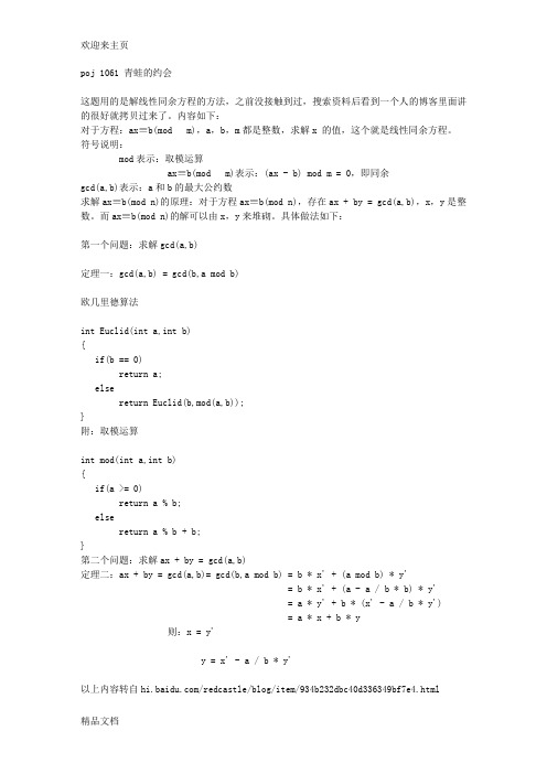
poj 1061 青蛙的约会这题用的是解线性同余方程的方法,之前没接触到过,搜索资料后看到一个人的博客里面讲的很好就拷贝过来了。
内容如下:对于方程:ax≡b(mod m),a,b,m都是整数,求解x 的值,这个就是线性同余方程。
符号说明:mod表示:取模运算ax≡b(mod m)表示:(ax - b) mod m = 0,即同余gcd(a,b)表示:a和b的最大公约数求解ax≡b(mod n)的原理:对于方程ax≡b(mod n),存在ax + by = gcd(a,b),x,y是整数。
而ax≡b(mod n)的解可以由x,y来堆砌。
具体做法如下:第一个问题:求解gcd(a,b)定理一:gcd(a,b) = gcd(b,a mod b)欧几里德算法int Euclid(int a,int b){if(b == 0)return a;elsereturn Euclid(b,mod(a,b));}附:取模运算int mod(int a,int b){if(a >= 0)return a % b;elsereturn a % b + b;}第二个问题:求解ax + by = gcd(a,b)定理二:ax + by = gcd(a,b)= gcd(b,a mod b) = b * x' + (a mod b) * y'= b * x' + (a - a / b * b) * y'= a * y' + b * (x' - a / b * y')= a * x + b * y则:x = y'y = x' - a / b * y'以上内容转自/redcastle/blog/item/934b232dbc40d336349bf7e4.html由这个可以得出扩展的欧几里德算法:int exGcd(int a, int b, int &x, int &y) {if(b == 0){x = 1;y = 0;return a;}int r = exGcd(b, a % b, x, y);int t = x;x = y;y = t - a / b * y;return r;}代码:#include<iostream>#include<cstdlib>#include<cstring>#include<cmath>using namespace std;__int64 mm,nn,xx,yy,l;__int64 c,d,x,y;__int64 modd(__int64 a, __int64 b){if(a>=0)return a%b;elsereturn a%b+b;}__int64 exGcd(__int64 a, __int64 b) {if(b==0){x=1;y=0;return a;}__int64 r=exGcd(b, a%b);__int64 t=x;x=y;y=t-a/b*y;return r;}int main(){scanf("%I64d %I64d %I64d %I64d %I64d",&xx,&yy,&mm,&nn,&l);if(mm>nn) //分情况{d=exGcd(mm-nn,l);c=yy-xx;}else{d=exGcd(nn-mm,l);c=xx-yy;}if(c%d != 0){printf("Impossible\n");return 0;}l=l/d;x=modd(x*c/d,l); ///取模函数要注意printf("%I64d\n",x);system("pause");return 0;}POJ 1142 SmithNumber题意:寻找最接近而且大于给定的数字的SmithNumber什么是SmithNumber?用sum(int)表示一个int的各位的和,那一个数i如果是SmithNumber,则sum(i) =sigma( sum(Pj )),Pj表示i的第j个质因数。
acm暑期练习7-递归练习等

1. 分解质因数根据数论的知识可知,任何一个合数都可以写成几个质数相乘的形式,这几个质数都叫做这个合数的质因数。
例如:24=2×2×2×3。
现在从键盘输入一个正整数,请编程输出它的所有质因数。
Input从键盘输入一个正整数n。
Output输出该整数的所有质因数。
Sample Input180Sample Output2 23 3 5解析:/*算术基本定理:任意一个大于1的正整数都可以分解成有限个素数的乘积,且分解是唯一的.质数就是1乘以它本身. 算术基本定理的最早证明是由欧几里得给出的。
任何一个大于1的自然数N,都可以唯一分解成有限个质数的乘积:N=(P1^a1)*(P2^a2)(P3^a3)......(Pn^an) , 这里P1<P2<P3...<Pn是质数,其诸方幂 ai 是正整数.这样的分解称为N 的标准分解式.*/#include<>void main(){int i,n;scanf("%d",&n);for(i=2;i<n;){if(n%i==0){printf("%d ",i);n=n/i;}elsei++;}printf("%d\n",n);}2. 计算正整数的划分数。
#include <iostream>using namespace std;int part(int n,int m){if (n<1||m<1)return 0;if (n==1||m==1)return 1;if (n<m)return part(n,n);if (n==m)return part(n,m-1)+1;return part(n,m-1)+part(n-m,m);}void main(){int n,m;cin>>n>>m;cout<<part(n,m)<<endl;}3求一个二位数的13次方后的最后三位数。
数论1(讲义)

数论 1 知识点严文兰1.符号说明:如无特别说明,下面出现的字母表示的数都是整数2.整数的离散型:整数a <b ⇔a +1 ≤b ,3.n 次方差公式:a n -b n = (a -b)(a n-1 +a n-2b ++b n-1 ) ,4.带余除法:设a, b是两个给定的整数,且b ≠0,则存在唯一一对整数q和r,满足a =qb +r, 0 ≤r <| b |(1)当r=0 时,a =qb ,那么就说a 可被b 整除,记作b | a ,且称a 是b 的倍数,b 是a 的约数(也可称为因数,除数),a 不能被b 整除就记作b /|a ,(2)如果a 为素数,且a n | b, a n+1 /| b, 那么记为a n || b(3)设m ≠ 0 ,如果a, b 被m 除的余数相同,即m | a -b ,则称a 同余于b 模m,b 是a 对模m 的剩余,记为a ≡b(mod m) ,此关系式称为模m 的同余式,不然,则称a 不同余于b 模m,记为a≡/b(mod m),5.整除的性质:(1)a | b, b| c ⇒a | c(2)a | b, a | c ⇒a | bx +cy ,特别地a | b, b | c ⇒a | b ±c ,(3)设m ≠ 0 ,那么a | b ⇔ma | mb ,(4)a | b ⇒b = 0 或| a |≤| b | ,所以 a | b, b | a ⇒b =±a(5)若(a, b) = 1,则a | c, b | c ⇔ab | c ,(6)m | a, m | b ⇒m | (a, b) ,(7)若(a, b) =1, ,则a | bc ⇔a | c ,(8)p 为素数,p | ab ⇒p | a 或p | b6.最大公约数与最小公倍数:同时整除a, b 的整数,叫a, b 的公约数,其中最大的那个,叫a, b 的最大公约数,记为(a, b) ,同样,同时整除a, b, , c 的最大整数,叫a, b, , c 的最大公约数,记为(a, b, , c) ,1 2 1 2同样,同时是 a , b ,, c 的倍数的整数,叫 a , b , , c 的公倍数,其中最小的正整数,叫a ,b , ,c 的最小公倍数,记为[a , b , , c ] 。
ACM数论方面十道基础题目详解
{
a=n-m;
b=l;
c=x-y;
r=gcd(a,b);
if(c%r)
{
printf("Impossible\n");
continue;
}
a/=r;
b/=r;
c/=r;
exgcd(a,b,k1,k2);
直接给出>
main()
{
int a,b,c,n;
scanf("%d%d%d",&a,&b,&c);
for(n=11;n<100;n++)
if(n%3==a&&n%5==b&&n%7==c)
printf("%d\n",n);
}
中国剩余定理思路代码:
inline int Gcd(int m,int n) //求最大公约数
{
if (m==0) return n;
return Gcd(n%m,m);
}
int main()
{
int n,a,b,g;
cin>>n;
while(n--)
{
cin>>a>>b;
g=Gcd(a,b);
cout<<g<<" "<<a*b/g<<endl;
if(n<=0)
n+=21252;
printf("%d\n",n);
北大暑期课程《回归分析》(Linear-Regression-Analysis)讲义1汇编

Class 1: Expectations, variances, and basics of estimationBasics of matrix (1)I. Organizational Matters(1)Course requirements:1)Exercises: There will be seven (7) exercises, the last of which is optional. Eachexercise will be graded on a scale of 0-10. In addition to the graded exercise, ananswer handout will be given to you in lab sections.2)Examination: There will be one in-class, open-book examination.(2)Computer software: StataII. Teaching Strategies(1) Emphasis on conceptual understanding.Yes, we will deal with mathematical formulas, actually a lot of mathematical formulas. But, I do not want you to memorize them. What I hope you will do, is to understand the logic behind the mathematical formulas.(2) Emphasis on hands-on research experience.Yes, we will use computers for most of our work. But I do not want you to become a computer programmer. Many people think they know statistics once they know how to run a statistical package. This is wrong. Doing statistics is more than running computer programs. What I will emphasize is to use computer programs to your advantage in research settings. Computer programs are like automobiles. The best automobile is useless unless someone drives it. You will be the driver of statistical computer programs.(3) Emphasis on student-instructor communication.I happen to believe in students' judgment about their own education. Even though I will be ultimately responsible if the class should not go well, I hope that you will feel part of the class and contribute to the quality of the course. If you have questions, do not hesitate to ask in class. If you have suggestions, please come forward with them. The class is as much yours as mine.Now let us get to the real business.III(1). Expectation and VarianceRandom Variable: A random variable is a variable whose numerical value is determined by the outcome of a random trial.Two properties: random and variable.A random variable assigns numeric values to uncertain outcomes. In a common language, "give a number". For example, income can be a random variable. There are many ways to do it. You can use the actual dollar amounts.In this case, you have a continuous random variable. Or you can use levels of income, such as high, median, and low. In this case, you have an ordinal random variable [1=high,2=median, 3=low]. Or if you are interested in the issue of poverty, you can have a dichotomous variable: 1=in poverty, 0=not in poverty.In sum, the mapping of numeric values to outcomes of events in this way is the essence of a random variable.Probability Distribution: The probability distribution for a discrete random variable X associates with each of the distinct outcomes x i(i = 1, 2,..., k) a probability P(X = x i).Cumulative Probability Distribution: The cumulative probability distribution for a discrete random variable X provides the cumulative probabilities P(X ≤ x) for all values x.Expected Value of Random Variable: The expected value of a discrete random variable X is denoted by E{X} and defined:E{X}=(x i)where: P(x i) denotes P(X = x i). The notation E{ } (read “expectation of”) is called the expectation operator.In common language, expectation is the mean. But the difference is that expectation is a concept for the entire population that you never observe. It is the result of the infinite number of repetitions. For example, if you toss a coin, the proportion of tails should be .5 in the limit. Or the expectation is .5. Most of the times you do not get the exact .5, but a number close to it.Conditional ExpectationIt is the mean of a variable conditional on the value of another random variable.Note the notation: E(Y|X).In 1996, per-capita average wages in three Chinese cities were (in RMB):Shanghai: 3,778Wuhan: 1,709Xi’an: 1,155Variance of Random Variable: The variance of a discrete random variable X is denoted by V{X} and defined:V{X}=i - E{X})2 P(x i)where: P(x i) denotes P(X = x i). The notation V{ }(read “variance of”) is called the variance operator.Since the variance of a random variable X is a weighted average of the squared deviations, (X - E{X})2 , it may be defined equivalently as an expected value: V{X} = E{(X - E{X})2}.An algebraically identical expression is: V{X} = E{X2} - (E{X})2.Standard Deviation of Random Variable: The positive square root of the variance of X is called the standard deviation of X and is denoted by σ{X}:σ{XThe notation σ{ } (read “standard deviation of”) is called the standard deviation operator. Standardized Random Variables: If X is a random variable with expected value E{X} and standard deviation σ{X}, then:Y=}{}{ X XEXσ-is known as the standardized form of random variable X.Covariance: The covariance of two discrete random variables X and Y is denoted by Cov{X,Y} and defined:Cov{X,Ywhere: P(x i, y jThe notation of Cov covariance operator.When X and Y are independent, Cov {X,Y} = 0.Cov {X,Y} = E{(X - E{X})(Y - E{Y})}; Cov {X,Y} = E{XY} - E{X}E{Y}(Variance is a special case of covariance.)Coefficient of Correlation: The coefficient of correlation of two random variables X and Y is denoted by ρ{X,Y} (Greek rho) and defined:where: σ{X} is the standard deviation of X; σ{Y} is the standard deviation of Y; Cov is the covariance of X and Y.Sum and Difference of Two Random Variables: If X and Y are two random variables, then the expected value and the variance of X + Y are as follows:Expected Value: E{X+Y} = E{X} + E{Y};Variance: V{X+Y} = V{X} + V{Y}+ 2 Cov(X,Y).If X and Y are two random variables, then the expected value and the variance of X - Y are as follows:Expected Value: E{X - Y} = E{X} - E{Y};Variance: V{X - Y} = V{X} + V{Y} - 2 Cov(X,Y).Sum of More Than Two Independent Random Variables: If T = X 1 + X 2 + ... + X s is the sumof s independent random variables, then the expected value and the variance of T are as follows:III(2). Properties of Expectations and Covariances:(1) Properties of Expectations under Simple Algebraic Operations)()(x bE a bX a E +=+This says that a linear transformation is retained after taking an expectation.bX a X +=*is called rescaling: a is the location parameter, b is the scale parameter.Special cases are:For a constant: a a E =)(For a different scale: )()(X E b bX E =, e.g., transforming the scale of dollars into the scale of cents.(2) Properties of Variances under Simple Algebraic Operations)()(2X V b bX a V =+This says two things: (1) Adding a constant to a variable does not change the variance of the variable; reason: the definition of variance controls for the mean of the variable[graphics]. (2) Multiplying a constant to a variable changes the variance of the variable by a factor of the constant squared; this is to easy prove, and I will leave it to you. This is the reason why we often use standard deviation instead of variance2x x σσ=is of the same scale as x.(3) Properties of Covariance under Simple Algebraic OperationsCov(a + bX, c + dY) = bd Cov(X,Y).Again, only scale matters, location does not.(4) Properties of Correlation under Simple Algebraic OperationsI will leave this as part of your first exercise:),(),(Y X dY c bX a ρρ=++That is, neither scale nor location affects correlation.IV: Basics of matrix.1. DefinitionsA. MatricesToday, I would like to introduce the basics of matrix algebra. A matrix is a rectangular array of elements arranged in rows and columns:11121211.......m n nm x x x x X x x ⎡⎤⎢⎥⎢⎥=⎢⎥⎢⎥⎣⎦Index: row index, column index.Dimension: number of rows x number of columns (n x m)Elements: are denoted in small letters with subscripts.An example is the spreadsheet that records the grades for your home work in the following way:Name 1st 2nd ....6thA 7 10 (9)B 6 5 (8)... ... ......Z 8 9 (8)This is a matrix.Notation: I will use Capital Letters for Matrices.B. VectorsVectors are special cases of matrices:If the dimension of a matrix is n x 1, it is a column vector:⎥⎥⎥⎥⎦⎤⎢⎢⎢⎢⎣⎡=n x x x x (21)If the dimension is 1 x m, it is a row vector:y' = | 1y 2y .... m y |Notation: small underlined letters for column vectors (in lecture notes)C. TransposeThe transpose of a matrix is another matrix with positions of rows and columns being exchanged symmetrically.For example: if⎥⎥⎥⎥⎦⎤⎢⎢⎢⎢⎣⎡=⨯nm n m m n x x x x x x X 12111211)( (1121112)()1....'...n m n m nm x x x x X x x ⨯⎡⎤⎢⎥⎢⎥=⎢⎥⎢⎥⎣⎦It is easy to see that a row vector and a column vector are transposes of each other. 2. Matrix Addition and SubtractionAdditions and subtraction of two matrices are possible only when the matrices have the same dimension. In this case, addition or subtraction of matrices forms another matrix whoseelements consist of the sum, or difference, of the corresponding elements of the two matrices.⎥⎥⎥⎥⎦⎤⎢⎢⎢⎢⎣⎡±±±±±=Y ±X mn nm n n m m y x y x y x y x y x (11)2121111111 Examples:⎥⎦⎤⎢⎣⎡=A ⨯4321)22(⎥⎦⎤⎢⎣⎡=B ⨯1111)22(⎥⎦⎤⎢⎣⎡=B +A =⨯5432)22(C 3. Matrix MultiplicationA. Multiplication of a scalar and a matrixMultiplying a scalar to a matrix is equivalent to multiplying the scalar to each of the elements of the matrix.11121211Χ...m n nm cx c cx cx ⎢⎥⎢⎥=⎢⎥⎢⎥⎣⎦ B. Multiplication of a Matrix by a Matrix (Inner Product)The inner product of matrix X (a x b) and matrix Y (c x d) exists if b is equal to c. The inner product is a new matrix with the dimension (a x d). The element of the new matrix Z is:c∑=kj ik ijy x zk=1Note that XY and YX are very different. Very often, only one of the inner products (XY and YX) exists.Example:⎥⎦⎤⎢⎣⎡=4321)22(x A⎥⎦⎤⎢⎣⎡=10)12(x BBA does not exist. AB has the dimension 2x1⎥⎦⎤⎢⎣⎡=42ABOther examples:If )53(x A , )35(x B , what is the dimension of AB? (3x3)If )53(x A , )35(x B , what is the dimension of BA? (5x5)If )51(x A , )15(x B , what is the dimension of AB? (1x1, scalar)If )53(x A , )15(x B , what is the dimension of BA? (nonexistent)4. Special MatricesA. Square Matrix)(n n A ⨯B. Symmetric MatrixA special case of square matrix.For )(n n A ⨯, ji ij a a =. All i, j .A' = AC. Diagonal MatrixA special case of symmetric matrix⎥⎥⎥⎥⎦⎢⎢⎢⎢⎣=X nn x x 0 (2211)D. Scalar Matrix0....0c c c c ⎡⎤⎢⎥⎢⎥=I ⎢⎥⎢⎥⎣⎦E. Identity MatrixA special case of scalar matrix⎥⎥⎥⎥⎦⎤⎢⎢⎢⎢⎣⎡=I 10 (101)Important: for r r A ⨯AI = IA = AF. Null (Zero) MatrixAnother special case of scalar matrix⎥⎥⎥⎥⎦⎤⎢⎢⎢⎢⎣⎡=O 00 (000)From A to E or F, cases are nested from being more general towards being more specific.G. Idempotent MatrixLet A be a square symmetric matrix. A is idempotent if....32=A =A =AH. Vectors and Matrices with elements being oneA column vector with all elements being 1,⎥⎥⎥⎥⎦⎤⎢⎢⎢⎢⎣⎡=⨯1......111r A matrix with all elements being 1, ⎥⎥⎥⎥⎦⎤⎢⎢⎢⎢⎣⎡=⨯1...1...111...11rr J Examples let 1 be a vector of n 1's: )1(1⨯n1'1 = )11(⨯n11' = )(n n J ⨯I. Zero VectorA zero vector is⎥⎥⎥⎥⎦⎤⎢⎢⎢⎢⎣⎡=⨯0....001r 5. Rank of a MatrixThe maximum number of linearly independent rows is equal to the maximum number of linearly independent columns. This unique number is defined to be the rank of the matrix. For example,⎥⎥⎥⎦⎤⎢⎢⎢⎣⎡=B 542211014321Because row 3 = row 1 + row 2, the 3rd row is linearly dependent on rows 1 and 2. The maximum number of independent rows is 2. Let us have a new matrix:⎥⎦⎤⎢⎣⎡=B 11014321*学习-----好资料更多精品文档 Singularity: if a square matrix A of dimension ()n n ⨯has rank n, the matrix is nonsingular. If the rank is less than n, the matrix is then singular.。
ACM竞赛中的数学方法初步

• 推论(Fermat小定理): 设p是素数, 若p 不能整除k, 则kp-1≡1(mod p)
• 初等数论的内容也是比较多的, 本次主要介 绍素数的测试, 数的整除性和跟同余有关的 一些知识.
素数测试
• 这是数论里的一个基本问题, 而且现代社会 应用也很广泛, 发展了很多算法. 首先要知 道下面的方法. • 给了一个数n, 从i=3开始到n的算术根以步 长2进行循环,如果n都不能整除i,那么n就 是一个素数 • 这种方法效率比较低, 判断一个数需要 O(n1/2)的时间复杂度
吃pizza的顺序
• 如果注意到n的大小只有10, 那么可以考虑 最稳妥的方法: 回溯搜索. 就是把所有可能 的排列情况按照字典顺序都搜索一遍, 找到 第一个可行的顺序就退出搜索. 如果搜索完 成之后都没有找到可行的取法, 说明没有可 行方法存在. 时间复杂度O(n!) • 具体方法, 如果你曾写过求迷宫的所有可行 路的程序, 应该很容易实现.
应用
• 用于计算向量夹角. • 判断两向量是否垂直 • 平面方程的向量形式: 平面方程 ax+by+cz=0(已通过移坐标轴去掉常数项), 令平面法向量n=(a,b,c), 点X(x,y,z), 则平面 方程记为n· X=0, 实际上, 如果平面过点P, 则方程为n· (X-P)=0.
应用(续)
• 以上是深度优先搜索的策略 • 实际上, 本题使用贪心策略也是可以AC的 (未能证明)
– 每次都选一块编号最小的可行的pizza片, 如果 某一步进行不下去, 就退出报告无可行取法. 时 间复杂度O(n2).
题外话
• 本题的操作比较复杂, 使用标准C++的算法 库配合复数类, 可以简化操作, 但是要求熟 悉上述工具.
最新北大暑期课程《回归分析》(Linear Regression Analysis)讲义1

Class 1: Expectations, variances, and basics of estimationBasics of matrix (1)I. Organizational Matters(1)Course requirements:1)Exercises: There will be seven (7) exercises, the last of which is optional. Eachexercise will be graded on a scale of 0-10. In addition to the graded exercise, ananswer handout will be given to you in lab sections.2)Examination: There will be one in-class, open-book examination.(2)Computer software: StataII. Teaching Strategies(1) Emphasis on conceptual understanding.Yes, we will deal with mathematical formulas, actually a lot of mathematical formulas. But, I do not want you to memorize them. What I hope you will do, is to understand the logic behind the mathematical formulas.(2) Emphasis on hands-on research experience.Yes, we will use computers for most of our work. But I do not want you to become a computer programmer. Many people think they know statistics once they know how to run a statistical package. This is wrong. Doing statistics is more than running computer programs. What I will emphasize is to use computer programs to your advantage in research settings. Computer programs are like automobiles. The best automobile is useless unless someone drives it. You will be the driver of statistical computer programs.(3) Emphasis on student-instructor communication.I happen to believe in students' judgment about their own education. Even though I will be ultimately responsible if the class should not go well, I hope that you will feel part of the class and contribute to the quality of the course. If you have questions, do not hesitate to ask in class. If you have suggestions, please come forward with them. The class is as much yours as mine.Now let us get to the real business.III(1). Expectation and VarianceRandom Variable: A random variable is a variable whose numerical value is determined by the outcome of a random trial.Two properties: random and variable.A random variable assigns numeric values to uncertain outcomes. In a common language, "give a number". For example, income can be a random variable. There are many ways to do it. You can use the actual dollar amounts.In this case, you have a continuous random variable. Or you can use levels of income, such as high, median, and low. In this case, you have an ordinal random variable [1=high,2=median, 3=low]. Or if you are interested in the issue of poverty, you can have a dichotomous variable: 1=in poverty, 0=not in poverty.In sum, the mapping of numeric values to outcomes of events in this way is theessence of a random variable.Probability Distribution: The probability distribution for a discrete random variable Xassociates with each of the distinct outcomes x i (i = 1, 2,..., k ) a probability P (X = x i ). Cumulative Probability Distribution: The cumulative probability distribution for a discreterandom variable X provides the cumulative probabilities P (X ≤ x ) for all values x .Expected Value of Random Variable: The expected value of a discrete random variable X isdenoted by E {X } and defined:E {X } = x i i k=∑1P (x i )where : P (x i ) denotes P (X = x i ). The notation E { } (read “expectation of”) is called theexpectation operator.In common language, expectation is the mean. But the difference is that expectation is a concept for the entire population that you never observe. It is the result of the infinitenumber of repetitions. For example, if you toss a coin, the proportion of tails should be .5 in the limit. Or the expectation is .5. Most of the times you do not get the exact .5, but a number close to it.Conditional ExpectationIt is the mean of a variable conditional on the value of another random variable.Note the notation: E(Y|X).In 1996, per-capita average wages in three Chinese cities were (in RMB):Shanghai: 3,778Wuhan: 1,709Xi ’an: 1,155Variance of Random Variable: The variance of a discrete random variable X is denoted by V {X } and defined:V {X } = i k =∑1(x i - E {X })2 P (x i )where : P (x i ) denotes P (X = x i ). The notation V { } (read “variance of”) is called the variance operator.Since the variance of a random variable X is a weighted average of the squared deviations,(X - E {X })2 , it may be defined equivalently as an expected value: V {X } = E {(X - E {X })2}. An algebraically identical expression is: V {X} = E {X 2} - (E {X })2.Standard Deviation of Random Variable: The positive square root of the variance of X is called the standard deviation of X and is denoted by σ{X }:σ {X } =V X {}The notation σ{ } (read “standard deviation of”) is called the standard deviation operator. Standardized Random Variables: If X is a random variable with expected value E {X } and standard deviation σ{X }, then:Y =}{}{X X E X σ-is known as the standardized form of random variable X .Covariance: The covariance of two discrete random variables X and Y is denoted by Cov {X,Y } and defined:Cov {X, Y } = ({})({})(,)xE X y E Y P x y i j i j j i --∑∑where: P (x i , y j ) denotes P Xx Y y i j (=⋂= ) The notation of Cov { , } (read “covariance of”) is called the covariance operator .When X and Y are independent, Cov {X, Y } = 0.Cov {X, Y } = E {(X - E {X })(Y - E {Y })}; Cov {X, Y } = E {XY } - E {X }E {Y }(Variance is a special case of covariance.)Coefficient of Correlation: The coefficient of correlation of two random variables X and Y isdenoted by ρ{X,Y } (Greek rho) and defined:ρσσ{,}{,}{}{}X Y Cov X Y X Y =where: σ{X } is the standard deviation of X; σ{Y } is the standard deviation of Y; Cov is the covariance of X and Y.Sum and Difference of Two Random Variables: If X and Y are two random variables, then the expected value and the variance of X + Y are as follows:Expected Value : E {X+Y } = E {X } + E {Y };Variance : V {X+Y } = V {X } + V {Y }+ 2 Cov (X,Y ).If X and Y are two random variables, then the expected value and the variance of X - Y are as follows:Expected Value : E {X - Y } = E {X } - E {Y };Variance : V {X - Y } = V {X } + V {Y } - 2 Cov (X,Y ).Sum of More Than Two Independent Random Variables: If T = X 1 + X 2 + ... + X s is the sumof s independent random variables, then the expected value and the variance of T are as follows:Expected Value: E T E X i i s {}{}==∑1; Variance: V T V X i i s {}{}==∑1III(2). Properties of Expectations and Covariances:(1) Properties of Expectations under Simple Algebraic Operations)()(x bE a bX a E +=+This says that a linear transformation is retained after taking an expectation.bX a X +=*is called rescaling: a is the location parameter, b is the scale parameter.Special cases are:For a constant: a a E =)(For a different scale: )()(X E b bX E =, e.g., transforming the scale of dollars into thescale of cents.(2) Properties of Variances under Simple Algebraic Operations)()(2X V b bX a V =+This says two things: (1) Adding a constant to a variable does not change the variance of the variable; reason: the definition of variance controls for the mean of the variable[graphics]. (2) Multiplying a constant to a variable changes the variance of the variable by a factor of the constant squared; this is to easy prove, and I will leave it to you. This is the reason why we often use standard deviation instead of variance2x x σσ=is of the same scale as x.(3) Properties of Covariance under Simple Algebraic OperationsCov(a + bX, c + dY) = bd Cov(X,Y).Again, only scale matters, location does not.(4) Properties of Correlation under Simple Algebraic OperationsI will leave this as part of your first exercise: ),(),(Y X dY c bX a ρρ=++That is, neither scale nor location affects correlation.IV: Basics of matrix.1. DefinitionsA. MatricesToday, I would like to introduce the basics of matrix algebra. A matrix is a rectangular array of elements arranged in rows and columns:11121211.......m n nm x x x x X x x ⎡⎤⎢⎥⎢⎥=⎢⎥⎢⎥⎣⎦Index: row index, column index.Dimension: number of rows x number of columns (n x m)Elements: are denoted in small letters with subscripts.An example is the spreadsheet that records the grades for your home work in the following way:Name 1st 2nd ....6thA 7 10 (9)B 6 5 (8)... ... ......Z 8 9 (8)This is a matrix.Notation: I will use Capital Letters for Matrices.B. VectorsVectors are special cases of matrices:If the dimension of a matrix is n x 1, it is a column vector:⎥⎥⎥⎥⎦⎤⎢⎢⎢⎢⎣⎡=n x x x x (21)If the dimension is 1 x m, it is a row vector: y' = | 1y 2y .... m y |Notation: small underlined letters for column vectors (in lecture notes)C. TransposeThe transpose of a matrix is another matrix with positions of rows and columns beingexchanged symmetrically.For example: if⎥⎥⎥⎥⎦⎤⎢⎢⎢⎢⎣⎡=⨯nm n m m n x x x x x x X 12111211)( (1121112)()1....'...n m n m nm x x x x X x x ⨯⎡⎤⎢⎥⎢⎥=⎢⎥⎢⎥⎣⎦It is easy to see that a row vector and a column vector are transposes of each other. 2. Matrix Addition and SubtractionAdditions and subtraction of two matrices are possible only when the matrices have the same dimension. In this case, addition or subtraction of matrices forms another matrix whoseelements consist of the sum, or difference, of the corresponding elements of the two matrices.⎥⎥⎥⎥⎦⎤⎢⎢⎢⎢⎣⎡±±±±±=Y ±X mn nm n n m m y x y x y x y x y x (11)2121111111 Examples:⎥⎦⎤⎢⎣⎡=A ⨯4321)22(⎥⎦⎤⎢⎣⎡=B ⨯1111)22(⎥⎦⎤⎢⎣⎡=B +A =⨯5432)22(C 3. Matrix MultiplicationA. Multiplication of a scalar and a matrixMultiplying a scalar to a matrix is equivalent to multiplying the scalar to each of the elements of the matrix.11121211Χ...m n nm cx c cx cx ⎢⎥⎢⎥=⎢⎥⎢⎥⎣⎦ B. Multiplication of a Matrix by a Matrix (Inner Product)The inner product of matrix X (a x b) and matrix Y (c x d) exists if b is equal to c. The inner product is a new matrix with the dimension (a x d). The element of the new matrix Z is:c∑=kj ik ijy x zk=1Note that XY and YX are very different. Very often, only one of the inner products (XY and YX) exists.Example:⎥⎦⎤⎢⎣⎡=4321)22(x A⎥⎦⎤⎢⎣⎡=10)12(x BBA does not exist. AB has the dimension 2x1⎥⎦⎤⎢⎣⎡=42ABOther examples:If )53(x A , )35(x B , what is the dimension of AB? (3x3)If )53(x A , )35(x B , what is the dimension of BA? (5x5)If )51(x A , )15(x B , what is the dimension of AB? (1x1, scalar)If )53(x A , )15(x B , what is the dimension of BA? (nonexistent)4. Special MatricesA. Square Matrix)(n n A ⨯B. Symmetric MatrixA special case of square matrix.For )(n n A ⨯, ji ij a a =. All i, j .A' = AC. Diagonal MatrixA special case of symmetric matrix⎥⎥⎥⎥⎦⎢⎢⎢⎢⎣=X nn x x 0 (2211)D. Scalar Matrix0....0c c c c ⎡⎤⎢⎥⎢⎥=I ⎢⎥⎢⎥⎣⎦E. Identity MatrixA special case of scalar matrix⎥⎥⎥⎥⎦⎤⎢⎢⎢⎢⎣⎡=I 10 (101)Important: for r r A ⨯AI = IA = AF. Null (Zero) MatrixAnother special case of scalar matrix⎥⎥⎥⎥⎦⎤⎢⎢⎢⎢⎣⎡=O 00 (000)From A to E or F, cases are nested from being more general towards being more specific.G. Idempotent MatrixLet A be a square symmetric matrix. A is idempotent if ....32=A =A =AH. Vectors and Matrices with elements being oneA column vector with all elements being 1,⎥⎥⎥⎥⎦⎤⎢⎢⎢⎢⎣⎡=⨯1 (111)r A matrix with all elements being 1, ⎥⎥⎥⎥⎦⎤⎢⎢⎢⎢⎣⎡=⨯1...1...111...11rr J Examples let 1 be a vector of n 1's: )1(1⨯n 1'1 = )11(⨯n11' = )(n n J ⨯I. Zero Vector A zero vector is ⎥⎥⎥⎥⎦⎤⎢⎢⎢⎢⎣⎡=⨯0 (001)r 5. Rank of a MatrixThe maximum number of linearly independent rows is equal to the maximum number oflinearly independent columns. This unique number is defined to be the rank of the matrix. For example,⎥⎥⎥⎦⎤⎢⎢⎢⎣⎡=B 542211014321 Because row 3 = row 1 + row 2, the 3rd row is linearly dependent on rows 1 and 2. The maximum number of independent rows is 2. Let us have a new matrix:⎥⎦⎤⎢⎣⎡=B 11014321* Singularity: if a square matrix A of dimension ()n n ⨯has rank n, the matrix is nonsingular. If the rank is less than n, the matrix is then singular.。
- 1、下载文档前请自行甄别文档内容的完整性,平台不提供额外的编辑、内容补充、找答案等附加服务。
- 2、"仅部分预览"的文档,不可在线预览部分如存在完整性等问题,可反馈申请退款(可完整预览的文档不适用该条件!)。
- 3、如文档侵犯您的权益,请联系客服反馈,我们会尽快为您处理(人工客服工作时间:9:00-18:30)。
hdu 3949 XOR
• 求n个int数里面x或的第k大值
• N有多大,基向量都不超过32个 • mod2高斯消元求出基向量就可以代表这 n个int的所有xor结果 • 将k分解二进制
筛素数
• 筛素数大家都会 • 初始2..n • 每次取出第一个没被删掉的元素p 必然是 素数 • 将p的倍数都删掉 • 复杂度:n/1 + n/2 + n/3 + n/5 + .. + n/p
ቤተ መጻሕፍቲ ባይዱ
• 化为裴蜀定理的一般情况,有解当且仅 当 gcd(b1, b2) | (a1-a2)
中国剩余定理的一般情况
• • • • 于是我们得到了一个初始的(u,v)记做(u0,v0) u*b1 + v*b2 = (a1-a2) 的所有解(u,v) 满足 u = u0 + tb2/gcd(b1,b2) v = v0 – tb1/gcd(b1,b2)
ACM中的数论
北京大学ACM队 李晔晨 lccycc@
/lccycc_acm
基本概念
• 模,同余 • 最大公约数和最小公倍数 • 素数,互素 • 正整数的素因数分解
本讲要点
• 扩展gcd与裴蜀定理
– 模线性方程 – 模线性方程组—中国剩余定理
• 高斯消元法
• 筛法线性求素数 • 欧拉函数
– – – – 当x≥ϕ (m)时,ax≡a(x mod ϕ(n)+ ϕ(n)) (mod n) 不需要互素 用途:计算a^b^c^d^e..的高阶幂次取模 (如何计算?)
POJ3696 The Luckiest number
• 题目大意:
– 定义只含有数字8的数为幸运数 – 给定正整数L,求L的所有倍数中最小的幸运数
扩展gcd与裴蜀定理
• 最大公约数:d = gcd(a,b) • 裴蜀定理:存在u,v使得 a*u + b*v = d • 裴蜀定理特例:若a,b互质,gcd(a,b) = 1 则存在u,v 使得 a*u + b*v = 1 • 设 a = pd, b = qd, 则p,q互质(为什么?) 裴蜀定理 pdu + qdv = d -> pu + qv = 1 转化为特例
中国剩余定理
• • • • • • • 设n组数(ai, bi), 其中bi两两互素 如果bi不是两两互素呢? 另一个角度看此问题 x = a1( mod b1) x = a2( mod b2) ->x + u*b1 = a1, x - v*b2 = a2 -> u*b1 + v*b2 = (a1-a2)
线性筛素数
• 一个元素会被删好多次。 • 如何优化成线性?
对每个素数p 考虑所有i, i的最小素因子>=p 将i*p去掉 如何代码实现?
• • • • • • • • • •
memset(Prime,0,sizeof(Prime)); memset(IsPrime,1,sizeof(IsPrime)); for (int i=2;i<=n;i++){ if (IsPrime[i]) Prime[num++] = i; for (int j=1;j<num && i*Prime[j]<=n;j++){ IsPrime[i*Prime[j]] = 0; if (i%Prime[j] == 0) break; } }
裴蜀定理的 证明
• • • • 直接构造出u,v au + bv = d (a-b)u + b(u+v) = d 令a’ = a%b, 令t使得a = b*t + a’
– t = [a/b]
• (a-tb)u + b(tu + v) = d • a’u + b(tu+v) = d • 令v’ = tu+v, 得到a’u + bv’ = d
扩展gcd算法
• 令v’ = tu+v, 得到a’u + bv’ = d • v = v’ – tu 若知道(u, v’)则可知道(u,v) int gcd(int a, int b){ return b==0?a:gcd(b,a%b); } int ex_gcd(int a,int b, int &u, int &v){ If (b == 0){ u = 1, v = 0; Return a; } int d = ex_gcd(b, a%b, v, u); v = v - a/b *u; return d; }
莫比乌斯函数的应用
• 求(u,v)对的互素对对数,1<=u,v<=n
– 比如 (2,3) (6,7)
• • • •
G(n) = n*n F(n)= [1..n]X[1..n] 中的互素对对数 要求f(n) 有G(n) = f d
d |n
• 算法思路:
– 设最终答案为x个8,则x满足(10x-1)*8/9≡0 (mod L) – 化简:10x≡1 (mod n),其中n=9L/gcd(9L,8) – 这是一个离散对数的问题,求解方法如下:
• 若gcd(10,n)>1,无解 • 若gcd(10,n)=1,由欧拉定理:10ϕ(n)≡1 (mod n)。可以证明, x为ϕ(n)的约数,从小到大枚举约数即可 • 10l≡1 (mod n) 则成立的最小 l 是ϕ (n)的约数 这个性质竞 赛中经常用到
1 k n 1 0 n pi , i j pi p j
i 1 k
n 1 else
g n f d f n g d n / d
d |n d |n
• 该函数也是积性函数 • 莫比乌斯反演
注意1这里反转 注意2这里容易溢出
模线性方程
• ax = d (mod b) abd 已知求x • 转化为ax + by = d 用扩展gcd求x,y
– 注意2容易溢出 – 在求x,y的中间步对其mod b处理
中国剩余定理
• 设n组数(ai, bi), 其中bi两两互素 • 求x使得
x = a1 mod b1 x = a2 mod b2 ... x = an mod bn
POJ2478 Farey Sequence
• 求所有分母不大于n的既约真分数个数
分母为x的既约真分数有ϕ(x)个 分母不大于n的既约真分数个数为ϕ(1)+ ϕ(2)+...+ ϕ(n) 如何快速求出ϕ(1), … ϕ(n)? 对ϕ(x),分解然后递推
莫比乌斯函数
• 设n=p1r1p2r2...pkrk
高斯消元法
• • • • • a11x1 + a12x2 + .. + a1nxn = b1 a21x1 + a22x2 + .. + a2nxn = b2 … am1 x1 + am2x2 + .. + amnxn = bm 求解<x1, x2, …xn> 一般m=n
• 如果是在mod p的线性空间下呢?(p素数)
欧拉函数
• • • • • ϕ (n) = 1..n中与n互质的数的个数 如何求ϕ (n)? 素因子展开+容斥原理 令n = p1r1p2r2...pkrk ϕ(n)=n*(1-1/p1)*(1-1/p2)*...*(1-1/pk)
– (为什么?)
欧拉定理
• 若a和n互质,则aϕ(n)≡1 (mod n) • 欧拉定理的推广形式
– (为什么?)
• x + u*b1 = a1 • x 的解空间为 a1 – u0b1 - t(b1b2)/gcd(b1b2)
= a1 - u0b1 - t*LCM(b1,b2)
中国剩余定理的一般情况
• x = a1 - u0b1 - t*LCM(b1,b2)
• 等价于:我们把前两个方程变成了一个 方程: • x = a1-u0b1 (mod LCM(b1,b2) ) • 每次方程数-1 继续这样消下去 就可以得 出x的可行解空间。 • 注意:扩展欧几里得算法给出的是一个 解空间!
中国剩余定理
• 令B = b1*b2*b3…*bn • 令ci = B/bi = b1*b2*..*b(i-1)*b(i+1)..*bn • 显然有ci 与bi互素,从而存在mi满足 mi*ci = bi (mod b) • x = a1b1m1 + a2b2m2 + …+anbnmn
– 为什么这个x是解? – 联想:拉格朗日插值公式!