组织经济学与管理学ch13 Biases in decision making
组织的经济学与管理学(英文)ch02 Positioning
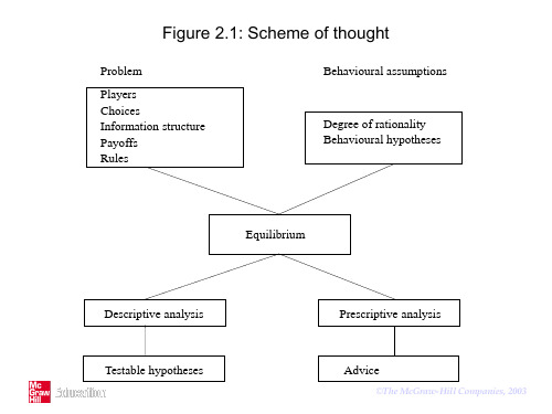
Strategy
A specification of an action/choice for each possible history/contingency/
situation which might occur, given the information structure. or
Specification of an action/choice for each observable history of the game.
situations
©The McGraw-Hill Companies, 2003
Non-cooperative game theory
A non-cooperative game consists of 5 ingredients: 1. Players 2. Actions 3. Payoffs 4. Information structure 5. Rules of the game
Extensive form
Frank
C
N
Cookie ?
R SR
Ann
S
Run ?
-11
-1 -10
0
-4
1 -5
0
©The McGraw-Hill Companies, 2003
Ann
(R, R) (R, S) (S, R) (S, S)
Frank
C (-11, -4) (-11, -4) (-1, 1) (-1, 1)
2. Actions / strategies
Environmental pollution game
Firm
P
C
Pollute ?
组织经济学与管理学ch12 Limited cognition and organisation-PPT精选文档75页

No
Increased
profit?
opportunities?
CEO
©The McGraw-Hill Companies, 2003
CEO
The CEO in a divisional structure decides to allocate as many means as
possible to division 1 in the future.
R|G|W|D
Conclusion: 3 partitions implies complexity 3.
©The McGraw-Hill Companies, 2003
Figure 12.1: Colour recognition capacities of different decision makers
©The McGraw-Hill Companies, 2003
Example
• Organisation consists of two divisions • Each division consists of two
managers • CEO only uses advice of each division • Divisions base their advice on
Fields
• Behavioural accounting • behavioural finance • Economic psychology / consumer
behaviour • Organisational behaviour • Strategic decision making
• A division reports negatively only when both local managers are negative
计量经济学导论CH13习题答案

CHAPTER 13TEACHING NOTESWhile this chapter falls under “Advanced Topics,” most of this chapter requires no more sophistication than the previous chapters. (In fact, I would argue that, with the possible exception of Section 13.5, this material is easier than some of the time series chapters.)Pooling two or more independent cross sections is a straightforward extension of cross-sectional methods. Nothing new needs to be done in stating assumptions, except possibly mentioning that random sampling in each time period is sufficient. The practically important issue is allowing for different intercepts, and possibly different slopes, across time.The natural experiment material and extensions of the difference-in-differences estimator is widely applicable and, with the aid of the examples, easy to understand.Two years of panel data are often available, in which case differencing across time is a simple way of removing g unobserved heterogeneity. If you have covered Chapter 9, you might compare this with a regression in levels using the second year of data, but where a lagged dependent variable is included. (The second approach only requires collecting information on the dependent variable in a previous year.) These often give similar answers. Two years of panel data, collected before and after a policy change, can be very powerful for policy analysis. Having more than two periods of panel data causes slight complications in that the errors in the differenced equation may be serially correlated. (However, the traditional assumption that the errors in the original equation are serially uncorrelated is not always a good one. In other words, it is not always more appropriate to used fixed effects, as in Chapter 14, than first differencing.) With large N and relatively small T, a simple way to account for possible serial correlation after differencing is to compute standard errors that are robust to arbitrary serial correlation and heteroskedasticity. Econometrics packages that do cluster analysis (such as Stata) often allow this by specifying each cross-sectional unit as its own cluster.108SOLUTIONS TO PROBLEMS13.1 Without changes in the averages of any explanatory variables, the average fertility rate fellby .545 between 1972 and 1984; this is simply the coefficient on y84. To account for theincrease in average education levels, we obtain an additional effect: –.128(13.3 – 12.2) ≈–.141. So the drop in average fertility if the average education level increased by 1.1 is .545+ .141 = .686, or roughly two-thirds of a child per woman.13.2 The first equation omits the 1981 year dummy variable, y81, and so does not allow anyappreciation in nominal housing prices over the three year period in the absence of an incinerator. The interaction term in this case is simply picking up the fact that even homes that are near the incinerator site have appreciated in value over the three years. This equation suffers from omitted variable bias.The second equation omits the dummy variable for being near the incinerator site, nearinc,which means it does not allow for systematic differences in homes near and far from the sitebefore the site was built. If, as seems to be the case, the incinerator was located closer to lessvaluable homes, then omitting nearinc attributes lower housing prices too much to theincinerator effect. Again, we have an omitted variable problem. This is why equation (13.9) (or,even better, the equation that adds a full set of controls), is preferred.13.3 We do not have repeated observations on the same cross-sectional units in each time period,and so it makes no sense to look for pairs to difference. For example, in Example 13.1, it is veryunlikely that the same woman appears in more than one year, as new random samples areobtained in each year. In Example 13.3, some houses may appear in the sample for both 1978and 1981, but the overlap is usually too small to do a true panel data analysis.β, but only13.4 The sign of β1 does not affect the direction of bias in the OLS estimator of1whether we underestimate or overestimate the effect of interest. If we write ∆crmrte i = δ0 +β1∆unem i + ∆u i, where ∆u i and ∆unem i are negatively correlated, then there is a downward biasin the OLS estimator of β1. Because β1 > 0, we will tend to underestimate the effect of unemployment on crime.13.5 No, we cannot include age as an explanatory variable in the original model. Each person inthe panel data set is exactly two years older on January 31, 1992 than on January 31, 1990. This means that ∆age i = 2 for all i. But the equation we would estimate is of the form∆saving i = δ0 + β1∆age i +…,where δ0 is the coefficient the year dummy for 1992 in the original model. As we know, whenwe have an intercept in the model we cannot include an explanatory variable that is constant across i; this violates Assumption MLR.3. Intuitively, since age changes by the same amount for everyone, we cannot distinguish the effect of age from the aggregate time effect.10913.6 (i) Let FL be a binary variable equal to one if a person lives in Florida, and zero otherwise. Let y90 be a year dummy variable for 1990. Then, from equation (13.10), we have the linear probability modelarrest = β0 + δ0y90 + β1FL + δ1y90⋅FL + u.The effect of the law is measured by δ1, which is the change in the probability of drunk driving arrest due to the new law in Florida. Including y90 allows for aggregate trends in drunk driving arrests that would affect both states; including FL allows for systematic differences between Florida and Georgia in either drunk driving behavior or law enforcement.(ii) It could be that the populations of drivers in the two states change in different ways over time. For example, age, race, or gender distributions may have changed. The levels of education across the two states may have changed. As these factors might affect whether someone is arrested for drunk driving, it could be important to control for them. At a minimum, there is the possibility of obtaining a more precise estimator of δ1 by reducing the error variance. Essentially, any explanatory variable that affects arrest can be used for this purpose. (See Section 6.3 for discussion.)SOLUTIONS TO COMPUTER EXERCISES13.7 (i) The F statistic (with 4 and 1,111 df) is about 1.16 and p-value ≈ .328, which shows that the living environment variables are jointly insignificant.(ii) The F statistic (with 3 and 1,111 df) is about 3.01 and p-value ≈ .029, and so the region dummy variables are jointly significant at the 5% level.(iii) After obtaining the OLS residuals, ˆu, from estimating the model in Table 13.1, we run the regression 2ˆu on y74, y76, …, y84 using all 1,129 observations. The null hypothesis of homoskedasticity is H0: γ1 = 0, γ2= 0, … , γ6 = 0. So we just use the usual F statistic for joint significance of the year dummies. The R-squared is about .0153 and F ≈ 2.90; with 6 and 1,122 df, the p-value is about .0082. So there is evidence of heteroskedasticity that is a function of time at the 1% significance level. This suggests that, at a minimum, we should compute heteroskedasticity-robust standard errors, t statistics, and F statistics. We could also use weighted least squares (although the form of heteroskedasticity used here may not be sufficient; it does not depend on educ, age, and so on).(iv) Adding y74⋅educ, , y84⋅educ allows the relationship between fertility and education to be different in each year; remember, the coefficient on the interaction gets added to the coefficient on educ to get the slope for the appropriate year. When these interaction terms are added to the equation, R2≈ .137. The F statistic for joint significance (with 6 and 1,105 df) is about 1.48 with p-value ≈ .18. Thus, the interactions are not jointly significant at even the 10% level. This is a bit misleading, however. An abbreviated equation (which just shows the coefficients on the terms involving educ) is110111kids= -8.48 - .023 educ + - .056 y74⋅educ - .092 y76⋅educ(3.13) (.054) (.073) (.071) - .152 y78⋅educ - .098 y80⋅educ - .139 y82⋅educ - .176 y84⋅educ .(.075) (.070) (.068) (.070)Three of the interaction terms, y78⋅educ , y82⋅educ , and y84⋅educ are statistically significant at the 5% level against a two-sided alternative, with the p -value on the latter being about .012. The coefficients are large in magnitude as well. The coefficient on educ – which is for the base year, 1972 – is small and insignificant, suggesting little if any relationship between fertility andeducation in the early seventies. The estimates above are consistent with fertility becoming more linked to education as the years pass. The F statistic is insignificant because we are testing some insignificant coefficients along with some significant ones.13.8 (i) The coefficient on y85 is roughly the proportionate change in wage for a male (female = 0) with zero years of education (educ = 0). This is not especially useful since we are not interested in people with no education.(ii) What we want to estimate is θ0 = δ0 + 12δ1; this is the change in the intercept for a male with 12 years of education, where we also hold other factors fixed. If we write δ0 = θ0 - 12δ1, plug this into (13.1), and rearrange, we getlog(wage ) = β0 + θ0y85 + β1educ + δ1y85⋅(educ – 12) + β2exper + β3exper 2 + β4union + β5female + δ5y85⋅female + u .Therefore, we simply replace y85⋅educ with y85⋅(educ – 12), and then the coefficient andstandard error we want is on y85. These turn out to be 0ˆθ = .339 and se(0ˆθ) = .034. Roughly, the nominal increase in wage is 33.9%, and the 95% confidence interval is 33.9 ± 1.96(3.4), or about 27.2% to 40.6%. (Because the proportionate change is large, we could use equation (7.10), which implies the point estimate 40.4%; but obtaining the standard error of this estimate is harder.)(iii) Only the coefficient on y85 differs from equation (13.2). The new coefficient is about –.383 (se ≈ .124). This shows that real wages have fallen over the seven year period, although less so for the more educated. For example, the proportionate change for a male with 12 years of education is –.383 + .0185(12) = -.161, or a fall of about 16.1%. For a male with 20 years of education there has been almost no change [–.383 + .0185(20) = –.013].(iv) The R -squared when log(rwage ) is the dependent variable is .356, as compared with .426 when log(wage ) is the dependent variable. If the SSRs from the regressions are the same, but the R -squareds are not, then the total sum of squares must be different. This is the case, as the dependent variables in the two equations are different.(v) In 1978, about 30.6% of workers in the sample belonged to a union. In 1985, only about 18% belonged to a union. Therefore, over the seven-year period, there was a notable fall in union membership.(vi) When y85⋅union is added to the equation, its coefficient and standard error are about -.00040 (se ≈ .06104). This is practically very small and the t statistic is almost zero. There has been no change in the union wage premium over time.(vii) Parts (v) and (vi) are not at odds. They imply that while the economic return to union membership has not changed (assuming we think we have estimated a causal effect), the fraction of people reaping those benefits has fallen.13.9 (i) Other things equal, homes farther from the incinerator should be worth more, so δ1 > 0. If β1 > 0, then the incinerator was located farther away from more expensive homes.(ii) The estimated equation islog()price= 8.06 -.011 y81+ .317 log(dist) + .048 y81⋅log(dist)(0.51) (.805) (.052) (.082)n = 321, R2 = .396, 2R = .390.ˆδ = .048 is the expected sign, it is not statistically significant (t statistic ≈ .59).While1(iii) When we add the list of housing characteristics to the regression, the coefficient ony81⋅log(dist) becomes .062 (se = .050). So the estimated effect is larger – the elasticity of price with respect to dist is .062 after the incinerator site was chosen – but its t statistic is only 1.24. The p-value for the one-sided alternative H1: δ1 > 0 is about .108, which is close to being significant at the 10% level.13.10 (i) In addition to male and married, we add the variables head, neck, upextr, trunk, lowback, lowextr, and occdis for injury type, and manuf and construc for industry. The coefficient on afchnge⋅highearn becomes .231 (se ≈ .070), and so the estimated effect and t statistic are now larger than when we omitted the control variables. The estimate .231 implies a substantial response of durat to the change in the cap for high-earnings workers.(ii) The R-squared is about .041, which means we are explaining only a 4.1% of the variation in log(durat). This means that there are some very important factors that affect log(durat) that we are not controlling for. While this means that predicting log(durat) would be very difficultˆδ: it could still for a particular individual, it does not mean that there is anything biased about1be an unbiased estimator of the causal effect of changing the earnings cap for workers’ compensation.(iii) The estimated equation using the Michigan data is112durat= 1.413 + .097 afchnge+ .169 highearn+ .192 afchnge⋅highearn log()(0.057) (.085) (.106) (.154)n = 1,524, R2 = .012.The estimate of δ1, .192, is remarkably close to the estimate obtained for Kentucky (.191). However, the standard error for the Michigan estimate is much higher (.154 compared with .069). The estimate for Michigan is not statistically significant at even the 10% level against δ1 > 0. Even though we have over 1,500 observations, we cannot get a very precise estimate. (For Kentucky, we have over 5,600 observations.)13.11 (i) Using pooled OLS we obtainrent= -.569 + .262 d90+ .041 log(pop) + .571 log(avginc) + .0050 pctstu log()(.535) (.035) (.023) (.053) (.0010) n = 128, R2 = .861.The positive and very significant coefficient on d90 simply means that, other things in the equation fixed, nominal rents grew by over 26% over the 10 year period. The coefficient on pctstu means that a one percentage point increase in pctstu increases rent by half a percent (.5%). The t statistic of five shows that, at least based on the usual analysis, pctstu is very statistically significant.(ii) The standard errors from part (i) are not valid, unless we thing a i does not really appear in the equation. If a i is in the error term, the errors across the two time periods for each city are positively correlated, and this invalidates the usual OLS standard errors and t statistics.(iii) The equation estimated in differences islog()∆= .386 + .072 ∆log(pop) + .310 log(avginc) + .0112 ∆pctsturent(.037) (.088) (.066) (.0041)n = 64, R2 = .322.Interestingly, the effect of pctstu is over twice as large as we estimated in the pooled OLS equation. Now, a one percentage point increase in pctstu is estimated to increase rental rates by about 1.1%. Not surprisingly, we obtain a much less precise estimate when we difference (although the OLS standard errors from part (i) are likely to be much too small because of the positive serial correlation in the errors within each city). While we have differenced away a i, there may be other unobservables that change over time and are correlated with ∆pctstu.(iv) The heteroskedasticity-robust standard error on ∆pctstu is about .0028, which is actually much smaller than the usual OLS standard error. This only makes pctstu even more significant (robust t statistic ≈ 4). Note that serial correlation is no longer an issue because we have no time component in the first-differenced equation.11311413.12 (i) You may use an econometrics software package that directly tests restrictions such as H 0: β1 = β2 after estimating the unrestricted model in (13.22). But, as we have seen many times, we can simply rewrite the equation to test this using any regression software. Write the differenced equation as∆log(crime ) = δ0 + β1∆clrprc -1 + β2∆clrprc -2 + ∆u .Following the hint, we define θ1 = β1 - β2, and then write β1 = θ1 + β2. Plugging this into the differenced equation and rearranging gives∆log(crime ) = δ0 + θ1∆clrprc -1 + β2(∆clrprc -1 + ∆clrprc -2) + ∆u .Estimating this equation by OLS gives 1ˆθ= .0091, se(1ˆθ) = .0085. The t statistic for H 0: β1 = β2 is .0091/.0085 ≈ 1.07, which is not statistically significant.(ii) With β1 = β2 the equation becomes (without the i subscript)∆log(crime ) = δ0 + β1(∆clrprc -1 + ∆clrprc -2) + ∆u= δ0 + δ1[(∆clrprc -1 + ∆clrprc -2)/2] + ∆u ,where δ1 = 2β1. But (∆clrprc -1 + ∆clrprc -2)/2 = ∆avgclr .(iii) The estimated equation islog()crime ∆ = .099 - .0167 ∆avgclr(.063) (.0051)n = 53, R 2 = .175, 2R = .159.Since we did not reject the hypothesis in part (i), we would be justified in using the simplermodel with avgclr . Based on adjusted R -squared, we have a slightly worse fit with the restriction imposed. But this is a minor consideration. Ideally, we could get more data to determine whether the fairly different unconstrained estimates of β1 and β2 in equation (13.22) reveal true differences in β1 and β2.13.13 (i) Pooling across semesters and using OLS givestrmgpa = -1.75 -.058 spring+ .00170 sat- .0087 hsperc(0.35) (.048) (.00015) (.0010)+ .350 female- .254 black- .023 white- .035 frstsem(.052) (.123) (.117) (.076)- .00034 tothrs + 1.048 crsgpa- .027 season(.00073) (0.104) (.049)n = 732, R2 = .478, 2R = .470.The coefficient on season implies that, other things fixed, an athlete’s term GPA is about .027 points lower when his/her sport is in season. On a four point scale, this a modest effect (although it accumulates over four years of athletic eligibility). However, the estimate is not statistically significant (t statistic ≈-.55).(ii) The quick answer is that if omitted ability is correlated with season then, as we know form Chapters 3 and 5, OLS is biased and inconsistent. The fact that we are pooling across two semesters does not change that basic point.If we think harder, the direction of the bias is not clear, and this is where pooling across semesters plays a role. First, suppose we used only the fall term, when football is in season. Then the error term and season would be negatively correlated, which produces a downward bias in the OLS estimator of βseason. Because βseason is hypothesized to be negative, an OLS regression using only the fall data produces a downward biased estimator. [When just the fall data are used, ˆβ = -.116 (se = .084), which is in the direction of more bias.] However, if we use just the seasonspring semester, the bias is in the opposite direction because ability and season would be positive correlated (more academically able athletes are in season in the spring). In fact, using just theβ = .00089 (se = .06480), which is practically and statistically equal spring semester gives ˆseasonto zero. When we pool the two semesters we cannot, with a much more detailed analysis, determine which bias will dominate.(iii) The variables sat, hsperc, female, black, and white all drop out because they do not vary by semester. The intercept in the first-differenced equation is the intercept for the spring. We have∆= -.237 + .019 ∆frstsem+ .012 ∆tothrs+ 1.136 ∆crsgpa- .065 seasontrmgpa(.206) (.069) (.014) (0.119) (.043) n = 366, R2 = .208, 2R = .199.Interestingly, the in-season effect is larger now: term GPA is estimated to be about .065 points lower in a semester that the sport is in-season. The t statistic is about –1.51, which gives a one-sided p-value of about .065.115(iv) One possibility is a measure of course load. If some fraction of student-athletes take a lighter load during the season (for those sports that have a true season), then term GPAs may tend to be higher, other things equal. This would bias the results away from finding an effect of season on term GPA.13.14 (i) The estimated equation using differences is∆= -2.56 - 1.29 ∆log(inexp) - .599 ∆log(chexp) + .156 ∆incshrvote(0.63) (1.38) (.711) (.064)n = 157, R2 = .244, 2R = .229.Only ∆incshr is statistically significant at the 5% level (t statistic ≈ 2.44, p-value ≈ .016). The other two independent variables have t statistics less than one in absolute value.(ii) The F statistic (with 2 and 153 df) is about 1.51 with p-value ≈ .224. Therefore,∆log(inexp) and ∆log(chexp) are jointly insignificant at even the 20% level.(iii) The simple regression equation is∆= -2.68 + .218 ∆incshrvote(0.63) (.032)n = 157, R2 = .229, 2R = .224.This equation implies t hat a 10 percentage point increase in the incumbent’s share of total spending increases the percent of the incumbent’s vote by about 2.2 percentage points.(iv) Using the 33 elections with repeat challengers we obtain∆= -2.25 + .092 ∆incshrvote(1.00) (.085)n = 33, R2 = .037, 2R = .006.The estimated effect is notably smaller and, not surprisingly, the standard error is much larger than in part (iii). While the direction of the effect is the same, it is not statistically significant (p-value ≈ .14 against a one-sided alternative).13.15 (i) When we add the changes of the nine log wage variables to equation (13.33) we obtain116117 log()crmrte ∆ = .020 - .111 d83 - .037 d84 - .0006 d85 + .031 d86 + .039 d87(.021) (.027) (.025) (.0241) (.025) (.025)- .323 ∆log(prbarr ) - .240 ∆log(prbconv ) - .169 ∆log(prbpris )(.030) (.018) (.026)- .016 ∆log(avgsen ) + .398 ∆log(polpc ) - .044 ∆log(wcon )(.022) (.027) (.030)+ .025 ∆log(wtuc ) - .029 ∆log(wtrd ) + .0091 ∆log(wfir )(0.14) (.031) (.0212)+ .022 ∆log(wser ) - .140 ∆log(wmfg ) - .017 ∆log(wfed )(.014) (.102) (.172)- .052 ∆log(wsta ) - .031 ∆log(wloc ) (.096) (.102) n = 540, R 2 = .445, 2R = .424.The coefficients on the criminal justice variables change very modestly, and the statistical significance of each variable is also essentially unaffected.(ii) Since some signs are positive and others are negative, they cannot all really have the expected sign. For example, why is the coefficient on the wage for transportation, utilities, and communications (wtuc ) positive and marginally significant (t statistic ≈ 1.79)? Higher manufacturing wages lead to lower crime, as we might expect, but, while the estimated coefficient is by far the largest in magnitude, it is not statistically different from zero (tstatistic ≈ –1.37). The F test for joint significance of the wage variables, with 9 and 529 df , yields F ≈ 1.25 and p -value ≈ .26.13.16 (i) The estimated equation using the 1987 to 1988 and 1988 to 1989 changes, where we include a year dummy for 1989 in addition to an overall intercept, isˆhrsemp ∆ = –.740 + 5.42 d89 + 32.60 ∆grant + 2.00 ∆grant -1 + .744 ∆log(employ ) (1.942) (2.65) (2.97) (5.55) (4.868)n = 251, R 2 = .476, 2R = .467.There are 124 firms with both years of data and three firms with only one year of data used, for a total of 127 firms; 30 firms in the sample have missing information in both years and are not used at all. If we had information for all 157 firms, we would have 314 total observations in estimating the equation.(ii) The coefficient on grant – more precisely, on ∆grant in the differenced equation – means that if a firm received a grant for the current year, it trained each worker an average of 32.6 hoursmore than it would have otherwise. This is a practically large effect, and the t statistic is very large.(iii) Since a grant last year was used to pay for training last year, it is perhaps not surprising that the grant does not carry over into more training this year. It would if inertia played a role in training workers.(iv) The coefficient on the employees variable is very small: a 10% increase in employ increases hours per employee by only .074. [Recall:∆≈ (.744/100)(%∆employ).] Thishrsempis very small, and the t statistic is also rather small.13.17. (i) Take changes as usual, holding the other variables fixed: ∆math4it = β1∆log(rexpp it) = (β1/100)⋅[ 100⋅∆log(rexpp it)] ≈ (β1/100)⋅( %∆rexpp it). So, if %∆rexpp it = 10, then ∆math4it= (β1/100)⋅(10) = β1/10.(ii) The equation, estimated by pooled OLS in first differences (except for the year dummies), is4∆ = 5.95 + .52 y94 + 6.81 y95- 5.23 y96- 8.49 y97 + 8.97 y98math(.52) (.73) (.78) (.73) (.72) (.72)- 3.45 ∆log(rexpp) + .635 ∆log(enroll) + .025 ∆lunch(2.76) (1.029) (.055)n = 3,300, R2 = .208.Taken literally, the spending coefficient implies that a 10% increase in real spending per pupil decreases the math4 pass rate by about 3.45/10 ≈ .35 percentage points.(iii) When we add the lagged spending change, and drop another year, we get4∆ = 6.16 + 5.70 y95- 6.80 y96- 8.99 y97 +8.45 y98math(.55) (.77) (.79) (.74) (.74)- 1.41 ∆log(rexpp) + 11.04 ∆log(rexpp-1) + 2.14 ∆log(enroll)(3.04) (2.79) (1.18)+ .073 ∆lunch(.061)n = 2,750, R2 = .238.The contemporaneous spending variable, while still having a negative coefficient, is not at all statistically significant. The coefficient on the lagged spending variable is very statistically significant, and implies that a 10% increase in spending last year increases the math4 pass rate118119 by about 1.1 percentage points. Given the timing of the tests, a lagged effect is not surprising. In Michigan, the fourth grade math test is given in January, and so if preparation for the test begins a full year in advance, spending when the students are in third grade would at least partly matter.(iv) The heteroskedasticity-robust standard error for log() ˆrexpp β∆is about 4.28, which reducesthe significance of ∆log(rexpp ) even further. The heteroskedasticity-robust standard error of 1log() ˆrexpp β-∆is about 4.38, which substantially lowers the t statistic. Still, ∆log(rexpp -1) is statistically significant at just over the 1% significance level against a two-sided alternative.(v) The fully robust standard error for log() ˆrexpp β∆is about 4.94, which even further reducesthe t statistic for ∆log(rexpp ). The fully robust standard error for 1log() ˆrexpp β-∆is about 5.13,which gives ∆log(rexpp -1) a t statistic of about 2.15. The two-sided p -value is about .032.(vi) We can use four years of data for this test. Doing a pooled OLS regression of ,1垐 on it i t r r -,using years 1995, 1996, 1997, and 1998 gives ˆρ= -.423 (se = .019), which is strong negative serial correlation.(vii) Th e fully robust “F ” test for ∆log(enroll ) and ∆lunch , reported by Stata 7.0, is .93. With 2 and 549 df , this translates into p -value = .40. So we would be justified in dropping these variables, but they are not doing any harm.。
组织经济学与管理学ch12 Limited cognition and organisation-75页PPT精品文档

X
X
X
X
©The McGraw-Hill Companies, 2003
Firm from an evolutionary perspective
Deel V: Tree
©The McGraw-Hill Companies, 2003
Making mistakes Forgetting
Limited reasoning capabilities
Partitioning
©The McGraw-Hill Companies, 2003
Deductive bounded rationality
How to optimally allocate a limited number of cognitive units in a complex problem?
Fields
• Behavioural accounting • behavioural finance • Economic psychology / consumer
behaviour • Organisational behaviour • Strategic decision making
©The McGraw-Hill Companies, 2003
Degree of rationality
Ratio of the cognitive capacities of the decision maker and the complexity of the problem.
©The McGraw-Hill Companies, 2003
Types of rationality
• Complete: ratio is 1 • Bounded: ratio between 0 and 1 • Procedural: ratio is (almost) 0
上海财经大学 斯蒂芬·P·罗宾斯《管理学》课件 ch13

江苏食堂承包大型服务商 常州食堂承包专家为您整理
13-2
学 习 目 标 (续)
• 你必须学习以下内容: – 说明流程再造与变革之间有怎样的联系。 – 了解减少员工压力的方法。 – 区分创造与创新。 – 解释组织应如何激励和培养创新。
江苏食堂承包大型服务商 常州食堂承包专家为您整理
13-3
什么是变革?
• 流程再造
– 一个组织完成各项活动所用方式的显著改变 – 始于活动的重设计
• 明确顾客需求 • 设计活动流程以最好地满足这些需求
– 要求管理者和员工的共同参与
13-20
持续质量改善计划与流程再造
持续质量改善 •持续而微小的变革 •巩固并改善 • 大多数需要回答“是什么” 流程再造
• 根本性的变革
6.欲速则不达;
7.因与果在时空上并不紧密相连; 8.寻找小而有效的杠杆解; 9.鱼和熊掌可以兼得; 10.系统具有整体性而不可分割;
11.没有绝对的内外。
13-30
管理变革中的问题(续)
• 处理员工的压力 – 什么是压力?
• 指个人面临机会、约束、或其需求渴望被满足时所 产生的一种不定的、身心不适的状态。 – 结果不确定却又很重要。 – 与约束和需求的联系特别紧密。 • 压力并不必然有害健康。 • 当以下条件满足,潜在压力会转变为现实压力: – 结果不确定 – 结果很重要
系统思考的道理说起来容易做起来难,所以,系统思考 不仅仅应该是一种理论的学习更主要的还是一种应用的学习, 也就是运用系统思考的法则进行修炼。
13-29
系统思考的修炼
1.今日的问题来自于昨日的解; 2.越用力推则系统反弹力越大;
3.恶化之前常先好转;
4.显而易见的解往往无效; 5.权宜之计的对策可能比问题更糟;
组织经济学与管理学ch14 Coordination-精品文档41页

Norwegian Dream Panamese Containership
Stop
Stop (3, -7)
Go
(2, -1)
Go (4, 3) (-5, -10)
©The McGraw-Hill Companies, 2003
One equilibrium emerges
Economics and Management of Organisations:
Co-ordination, Motivation and Strategy
Chapter 14
Coordination
George Hendrikse
©The McGraw-Hill Companies, 2003
There are many coordination mechanisms / devices which might resolve the coordination problem.
©The McGraw-Hill Companies, 2003
Criteria for evaluating coordination devices / mechanisms) value of the design variable. 3. Yes, conductor is very flexible
©The McGraw-Hill Companies, 2003
Surplus maximising choice
Conductor
©The McGraw-Hill Companies, 2003
Example: Norwegian Dream
©The McGraw-Hill Companies, 2003
组织经济学与管理学ch02 Positioning

Subgame perfect equilibrium
To be used when there is complete information.
©The McGraw-Hill Companies, 2003
Cookie extraction game
N (-10, -5) (0, 0) (-10, -5) (0,0)
©The McGraw-Hill Companies, 2003
Nash equilibria
• Frank: C • Ann: (S, R) and • Frank: N • Ann: (R, S) and • Frank: N • Ann: (S,S)
P
C
I
NI
Firm
Government
N
-1
40
0
3
0 -2
0
©The McGraw-Hill Companies, 2003
The oval represents an information set.
Government does not know which action is taken by the firm when it
©The McGraw-Hill Companies, 2003
Game theory
A unified analytical structure for studying all situations of conflict and cooperation
or A tool for modelling multiperson decision
Opportunistic
微观经济学(平狄克鲁宾费尔德)第六版课后答案--微观经济学 英文原版-CH13PINDYCK

Chapter 13
8ห้องสมุดไป่ตู้
Noncooperative vs. Cooperative Games
“The strategy design is based on understanding your opponent’s point of view, and (assuming your opponent is rational) deducing how he or she is likely to respond to your actions.” (Text, p. 475)
Typically bid more for the dollar when faced with loss as second highest bidder
Chapter 13
10
Acquiring a Company
Scenario
Company A: The Acquirer Company T: The Target A will offer cash for all of T’s shares
Chapter 13
7
Noncooperative vs. Cooperative Games
Noncooperative Game
Negotiation and enforcement of binding contracts between players is not possible
Buyer and seller negotiating the price of a good or service or a joint venture by two firms (i.e., Microsoft and Apple) Binding contracts are possible
- 1、下载文档前请自行甄别文档内容的完整性,平台不提供额外的编辑、内容补充、找答案等附加服务。
- 2、"仅部分预览"的文档,不可在线预览部分如存在完整性等问题,可反馈申请退款(可完整预览的文档不适用该条件!)。
- 3、如文档侵犯您的权益,请联系客服反馈,我们会尽快为您处理(人工客服工作时间:9:00-18:30)。
Laoften exaggerate the representativeness of a small sample.
©The McGraw-Hill Companies, 2003
©The McGraw-Hill Companies, 2003
3. Melioration
Herrnstein & Prelec (1992)
©The McGraw-Hill Companies, 2003
People (and animals) have the tendency to focus on today’s costs and
Striking information gets too much weight in the decision process of people.
©The McGraw-Hill Companies, 2003
Prospect theory
• Asymmetry between gains and losses • Reference point
decision processes.
©The McGraw-Hill Companies, 2003
1. Procrastination
Postpone - starting a healthy diet - starting a new project - killing a bad performing project - start studying for an exam
• changing the choice possibilities • structure the amount and nature of
information
©The McGraw-Hill Companies, 2003
Short term focus
Current costs and benefits receive a disproportional amount of attention in
Figure 13.2: Tendencies in decision making
Decision making dimension
Time Distance
Emphasis in actual decision making
Toomuch Toolittle
Nearfuture Distant future
decisions • job rotation (to limit overcommitment
to project)
©The McGraw-Hill Companies, 2003
Make results visible
• clear figures • step-by-step plan
©The McGraw-Hill Companies, 2003
characteristics of the situation.
©The McGraw-Hill Companies, 2003
2. Obedience
‘Befehl ist befehl’
©The McGraw-Hill Companies, 2003
Milgram experiments
A series of small, escalating concessions establishes an incredible obedience.
Economics and Management of Organisations:
Co-ordination, Motivation and Strategy
Chapter 13
Biases in decision making
George Hendrikse
©The McGraw-Hill Companies, 2003
represented.
©The McGraw-Hill Companies, 2003
Reference point
Most people are often more sensitive to how the current
situation differs from to a reference point, than to the actual
©The McGraw-Hill Companies, 2003
Framing
The choices / preferences of people are often not robust w.r.t.
the way in which choice possibilities / alternatives are
Small
Large
Result
Success
Failure
©The McGraw-Hill Companies, 2003
anisational measures
• changing the costs and / or benefits of the choice possibilities
benefits of current choices, without taking future consequences of these
choices into account.
©The McGraw-Hill Companies, 2003
Shortsightedness
• Distance • Interest / background • Probability of certain events occurring
©The McGraw-Hill Companies, 2003
Organisational responses
• pose a deadline for profitability • punish admitting mistakes mildly • allow credible excuses • separate starting and finishing