stata使用手册

合集下载

Stata 使用手册说明书

1Read this—it will helpContents1.1Getting Started with Stata1.2The User’s Guide and the Reference manuals1.2.1PDF manuals1.2.1.1Video example1.2.2Example datasets1.2.2.1Video example1.2.3Cross-referencing1.2.4The index1.2.5The subject table of contents1.2.6Typography1.2.7Vignette1.3What’s new1.4References12[U]1Read this—it will helpThe Stata Documentation consists of the following manuals:[GSM]Getting Started with Stata for Mac[GSU]Getting Started with Stata for Unix[GSW]Getting Started with Stata for Windows[U]Stata User’s Guide[R]Stata Base Reference Manual[ADAPT]Stata Adaptive Designs:Group Sequential Trials Reference Manual[BAYES]Stata Bayesian Analysis Reference Manual[BMA]Stata Bayesian Model Averaging Reference Manual[CAUSAL]Stata Causal Inference and Treatment-Effects Estimation Reference Manual[CM]Stata Choice Models Reference Manual[D]Stata Data Management Reference Manual[DSGE]Stata Dynamic Stochastic General Equilibrium Models Reference Manual[ERM]Stata Extended Regression Models Reference Manual[FMM]Stata Finite Mixture Models Reference Manual[FN]Stata Functions Reference Manual[G]Stata Graphics Reference Manual[IRT]Stata Item Response Theory Reference Manual[LASSO]Stata Lasso Reference Manual[XT]Stata Longitudinal-Data/Panel-Data Reference Manual[META]Stata Meta-Analysis Reference Manual[ME]Stata Multilevel Mixed-Effects Reference Manual[MI]Stata Multiple-Imputation Reference Manual[MV]Stata Multivariate Statistics Reference Manual[PSS]Stata Power,Precision,and Sample-Size Reference Manual[P]Stata Programming Reference Manual[RPT]Stata Reporting Reference Manual[SP]Stata Spatial Autoregressive Models Reference Manual[SEM]Stata Structural Equation Modeling Reference Manual[SVY]Stata Survey Data Reference Manual[ST]Stata Survival Analysis Reference Manual[TABLES]Stata Customizable Tables and Collected Results Reference Manual[TS]Stata Time-Series Reference Manual[I]Stata Index[M]Mata Reference ManualIn addition,installation instructions may be found in the Installation Guide.[U]1Read this—it will help3 1.1Getting Started with StataThere are three Getting Started manuals:[GSM]Getting Started with Stata for Mac[GSU]Getting Started with Stata for Unix[GSW]Getting Started with Stata for Windows1.Learn how to use Stata—read the Getting Started(GSM,GSU,or GSW)manual.2.Now turn to the other manuals;see[U]1.2The User’s Guide and the Reference manuals.1.2The User’s Guide and the Reference manualsThe User’s Guide is divided into three sections:Stata basics,Elements of Stata,and Advice.The table of contents lists the chapters within each of these sections.Click on the chapter titles to see the detailed contents of each chapter.The Guide is full of a lot of useful information about Stata;we recommend that you read it.If you only have time,however,to read one or two chapters,then read[U]11Language syntax and [U]12Data.The other manuals are the Reference manuals.The Stata Reference manuals are each arranged like an encyclopedia—alphabetically.Look at the Base Reference Manual.Look under the name ofa command.If you do notﬁnd the command,look in the subject index in[I]Stata Index.A fewcommands are so closely related that they are documented together,such as ranksum and median, which are both documented in[R]ranksum.Not all the entries in the Base Reference Manual are Stata commands;some contain technical information,such as[R]Maximize,which details Stata’s iterative maximization process,or[R]Error messages,which provides information on error messages and return codes.Like an encyclopedia,the Reference manuals are not designed to be read from cover to cover.When you want to know what a command does,complete with all the details,qualiﬁcations,and pitfalls,or when a command produces an unexpected result,read its description.Each entry is written at the level of the command.The descriptions assume that you have little knowledge of Stata’s features when they are explaining simple commands,such as those for using and saving data.For more complicated commands,they assume that you have aﬁrm grasp of Stata’s other features.If a Stata command is not in the Base Reference Manual,you canﬁnd it in one of the other Reference manuals.The titles of the manuals indicate the types of commands that they contain.The Programming Reference Manual,however,contains commands not only for programming Stata but also for manipulating matrices(not to be confused with the matrix programming language described in the Mata Reference Manual).1.2.1PDF manualsEvery copy of Stata comes with Stata’s complete PDF documentation.The PDF documentation may be accessed from within Stata by selecting Help>PDF documentation.Even more convenient,every helpﬁle in Stata links to the equivalent manual entry.If you are reading help regress,simply click on(View complete PDF manual entry)below the title of the helpﬁle to go directly to the[R]regress manual entry.We provide some tips for viewing Stata’s PDF documentation at https:///support/ faqs/resources/pdf-documentation-tips/.4[U]1Read this—it will help1.2.1.1Video examplePDF documentation in Stata1.2.2Example datasetsVarious examples in this manual use what is referred to as the automobile dataset,auto.dta.We have created a dataset on the prices,mileages,weights,and other characteristics of74automobiles and have saved it in aﬁle called auto.dta.(These data originally came from the April1979issue of Consumer Reports and from the United States Government EPA statistics on fuel consumption;they were compiled and published by Chambers et al.[1983].)In our examples,you will often see us type.use https:///data/r18/autoWe include the auto.dtaﬁle with Stata.If you want to use it from your own computer rather than via the Internet,you can type.sysuse autoSee[D]sysuse.You can also access auto.dta by selecting File>Example datasets...,clicking on Example datasets installed with Stata,and clicking on use beside the auto.dtaﬁlename.There are many other example datasets that ship with Stata or are available over the web.Here isa partial list of the example datasets included with Stata:auto.dta1978automobile databplong.dta Fictional blood-pressure data,long formbpwide.dta Fictional blood-pressure data,wide formcancer.dta Patient survival in drug trialcensus.dta1980Census data by statecitytemp.dta U.S.city temperature dataeduc99gdp.dta Education and gross domestic productgnp96.dta U.S.gross national product,1967–2002lifeexp.dta1998life expectancynetwork1.dta Fictional network diagram datanlsw88.dta1988U.S.National Longitudinal Survey of Young Women(NLSW),extractpop2000.dta2000U.S.Census population,extractsandstone.dta Subsea elevation of Lamont sandstone in an area of Ohiosp500.dta S&P500historic datasurface.dta NOAA sea surface temperaturetsline1.dta Simulated time-series datauslifeexp.dta U.S.life expectancy,1900–1999voter.dta1992U.S.presidential voter dataAll of these datasets may be used or described from the Example datasets...menu listing.Even more example datasets,including most of the datasets used in the reference manuals,are available at the Stata Press website(https:///data/).You can download the datasets with your browser,or you can use them directly from the Stata command line:.use https:///data/r18/nlswork[U]1Read this—it will help5An alternative to the use command for these example datasets is webuse.For example,typing .webuse nlsworkis equivalent to the above use command.For more information,see[D]webuse.1.2.2.1Video exampleExample datasets included with Stata1.2.3Cross-referencingThe Getting Started manual,the User’s Guide,and the Reference manuals cross-reference each other.[R]regress[D]reshape[XT]xtregTheﬁrst is a reference to the regress entry in the Base Reference Manual,the second is a reference to the reshape entry in the Data Management Reference Manual,and the third is a reference to the xtreg entry in the Longitudinal-Data/Panel-Data Reference Manual.[GSW]B Advanced Stata usage[GSM]B Advanced Stata usage[GSU]B Advanced Stata usageare instructions to see the appropriate section of the Getting Started with Stata for Windows,Getting Started with Stata for Mac,or Getting Started with Stata for Unix manual.1.2.4The indexThe Stata Index contains a combined index for all the manuals.Toﬁnd information and commands quickly,you can use Stata’s search command;see[R]search.At the Stata command prompt,type search geometric mean.search searches Stata’s keyword database and the Internet toﬁnd more commands and extensions for Stata written by Stata users.1.2.5The subject table of contentsA subject table of contents for the User’s Guide and all the Reference manuals is located in theStata Index.This subject table of contents may also be accessed by clicking on Contents in the PDF bookmarks.1.2.6TypographyWe mix the ordinary typeface that you are reading now with a typewriter-style typeface that looks like this.When something is printed in the typewriter-style typeface,it means that something is a command or an option—it is something that Stata understands and something that you might actually type into your computer.Differences in typeface are important.If a sentence reads,“You could list the result...”,it is just an English sentence—you could list the result,but the sentence provides no clue as to how you might actually do that.On the other hand,if the sentence reads,“You could list the result...”,it is telling you much more—you could list the result,and you could do that by using the list command.6[U]1Read this—it will helpWe will occasionally lapse into periods of inordinate cuteness and write,“We describe d the data and then list ed the data.”You get the idea.describe and list are Stata commands.We purposely began the previous sentence with a lowercase letter.Because describe is a Stata command,it must be typed in lowercase letters.The ordinary rules of capitalization are temporarily suspended in favor of preciseness.We also mix in words printed in italic type,such as“To perform the rank-sum test,type ranksum varname,by(groupvar)”.Italicized words are not supposed to be typed;instead,you are to substitute another word for them.We would also like users to note our rule for punctuation of quotes.We follow a rule that is often used in mathematics books and British literature.The punctuation mark at the end of the quote is included in the quote only if it is a part of the quote.For instance,the pleased Stata user said she thought that Stata was a“very powerful program”.Another user simply said,“I love Stata.”In this manual,however,there is little dialogue,and we follow this rule to precisely clarify what you are to type,as in,type“cd c:”.The period is outside the quotation mark because you should not type the period.If we had wanted you to type the period,we would have included two periods at the end of the sentence:one inside the quotation and one outside,as in,type“the orthogonal polynomial operator,p.”.We have tried not to violate the other rules of English.If youﬁnd such violations,they were unintentional and resulted from our own ignorance or carelessness.We would appreciate hearing about them.We have heard from Nicholas J.Cox of the Department of Geography at Durham University,UK, and express our appreciation.His efforts have gone far beyond dropping us a note,and there is no way with words that we can fully express our gratitude.1.2.7VignetteIf you look,for example,at the entry[R]brier,you will see a brief biographical vignette of Glenn Wilson Brier(1913–1998),who did pioneering work on the measures described in that entry.A few such vignettes were added without fanfare in the Stata8manuals,just for interest,and many more were added in Stata9,and even more have been added in each subsequent release.A vignette could often appropriately go in several entries.For example,George E.P.Box deserves to be mentioned in entries other than[TS]arima,such as[R]boxcox.However,to save space,each vignette is given once only,and an index of all vignettes is given in the Stata Index.Most of the vignettes were written by Nicholas J.Cox,Durham University,and were compiled using a wide range of reference books,articles in the literature,Internet sources,and information from individuals.Especially useful were the dictionaries of Upton and Cook(2014)and Everitt and Skrondal(2010)and the compilations of statistical biographies edited by Heyde and Seneta(2001) and Johnson and Kotz(1997).Of these,only theﬁrst provides information on people living at the time of publication.1.3What’s newThere are a lot of new features in Stata18.For a thorough overview of the most important new features,visithttps:///new-in-stata/[U]1Read this—it will help7 For a brief overview of all the new features that were added with the release of Stata18,in Stata type.help whatsnew17to18Stata is continually being updated.For a list of new features that have been added since the release of Stata18,in Stata type.help whatsnew181.4ReferencesChambers,J.M.,W.S.Cleveland,B.Kleiner,and P.A.Tukey.1983.Graphical Methods for Data Analysis.Belmont, CA:Wadsworth.Everitt, B.S.,and A.Skrondal.2010.The Cambridge Dictionary of Statistics.4th ed.Cambridge:Cambridge University Press.Gould,W.W.2014.Putting the Stata Manuals on your iPad.The Stata Blog:Not Elsewhere Classiﬁed./2014/10/28/putting-the-stata-manuals-on-your-ipad/.Heyde,C.C.,and E.Seneta,ed.2001.Statisticians of the Centuries.New York:Springer.Johnson,N.L.,and S.Kotz,ed.1997.Leading Personalities in Statistical Sciences:From the Seventeenth Century to the Present.New York:Wiley.Pinzon,E.,ed.2015.Thirty Years with Stata:A Retrospective.College Station,TX:Stata Press.Upton,G.J.G.,and I.T.Cook.2014.A Dictionary of Statistics.3rd ed.Oxford:Oxford University Press.Stata,Stata Press,and Mata are registered trademarks of StataCorp LLC.Stata andStata Press are registered trademarks with the World Intellectual Property Organization®of the United Nations.Other brand and product names are registered trademarks ortrademarks of their respective companies.Copyright c 1985–2023StataCorp LLC,College Station,TX,USA.All rights reserved.。

STATA基本操作入门

8.相关系数
• 如果要显示PL,PF两个变量的相关系数 • 方法：pwcorr pl pf
整理PP数
• 方法：pwcorr pl pf pk
整理PPT课件
15
8.1 相关系数
• 如果要显示PL,PF,PK三个变量之间的相关系数，并显示显著性水平
• 保存该图：输入graph save scatter2
整理PPT课件
22
9.6 图像合并展示
• 将线性拟合和二次拟合这两个图像在一起展示
• 方法:输入graph combine scatter1.gph scatter2.gph
整理PPT课件
23
此课件下载可自行编辑修改，此课件供参考！部分内容来源于网络，如有侵权请与我联系删除！感谢你的观看！
整理PPT课件
18
9.3 画图：散点图
整理PPT课件
19
9.3.1 散点图改进
• 定义新变量值n来表示第n个观测值： • 方法：gen n=_n （_n表示第n个观测值） • 使散点图显示对应的观测值： • 方法：scatter tc q,mlabel(n) mlabpos(6)
整理PPT课件
20
• 展示变量q的样本容量，平均值，标准差，最小值，最大值
整理PPT课件
9
6.2查看变量的统计特征
• 如果要查看满足q≥10000的子样本的统计指标。方法：输入summarize q if q >=10000
• 或者su q if q >=10000
整理PPT课件
10
6.3 查看变量的统计特征
Properties: 性质窗口，
显示当前数
据文件和变量的性质

stata入门教程

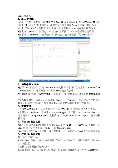
Stata 快速入门1、Stata的窗口•在最上方有一排菜单，即“File Edit Data Graphics Statistics User Window Help”。

•左上“Review”（历史窗口）：此窗口记录着自启动Stata以来执行过的命令。

•右上“Variables”（变量窗口）：此窗口记录着目前Stata内存中的所有变量。

•正上方“Results”（结果窗口）：此窗口显示执行Stata命令后的输出结果。

•正下方“Command”（命令窗口）：在此窗口输入想要执行的Stata命令。

2、将数据导入Stata•打开Stata软件后，点击Data Editor(Edit)图标（也可以点击菜单“Window”→“Data Editor”），即可打开一个类似Excel的空白表格。

•用Excel打开文件“nerlove.xls”，复制文件中的所有数据，并粘贴到Data Editor 中。

•导入数据的另一方法是，点击菜单“File”→“Import”，然后导入各种格式的数据。

但这种方法有时不如直接从Excel表中粘贴数据来得方便直观。

3、变量窗口•关闭Data Editor后，即会看到右上方的“Variables”窗口出现了5个变量：•分别为tc（total cost，总成本），q（total output, 总产量），pl（price of labor，小时工资率），pf（price of fuel，燃料价格），与pk（user cost of capital，资本的租赁价格。

4、存为dta数据文件•此时，可以点击Save图标（也可以点击菜单“File”→“Save”），将数据存为Stata格式的文件（扩展名为dta），比如nerlove.dta。

•以后就可以用Stata直接打开这个数据集了（不需要再从Excel表中粘贴过来）。

5、打开dta数据文件打开的方式有三种：1.点击Open图标（也可以点击菜单“File”→“Open”），然后寻找要打开的dta 文件的位置。

stata使用手册

STATA基本入门前言STATA是一个十分好用而且简单的统计软件包，透过轻松的数据输入方式，而且简单的指令，即可执行一般在计量经济学上常用的计量模型。

除了计量模型外，STATA的软件包中也可执行统计学中的估计和检定，甚至是多变量分析中的各项分析工具。

因此，STATA可以说是一个相当强而有力的统计软件。

一、安装STATA所须的内存容量不大，只有4.03MB。

此外，安装也相当简单，只要在〝SETUP〞上点两下，安装完成后再分别输入”Sn”、”Code”和”Key”即可开始使用。

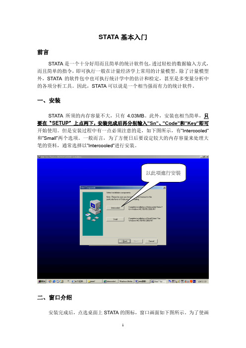
但是安装过程中有一点必须注意的是，如下图所示，有”Intercooled”和”Small”两个选项。

一般而言，为了方便日后要设定较大的内存容量来处理大笔的资料，通常选择以”Intercooled”进行安装。

以此項進行安裝二、窗口介绍安装完成后，点选桌面上STATA的图标，窗口画面如下图所示。

为了使画面美观，我们可以将画面拉到自己喜欢的地方，如下图所示。

为了保存这个窗口画面，我们必须点选工具列上的”Prefs”下的”Save Windowing Preferences”。

如此一来，以后开启STATA 时都会以此窗口画面呈现。

接下来，我们依序介绍四个窗口的功用：左上─Review：此一窗口用于记录在开启STATA后所执行过的所有指令。

因此，若欲使用重复的指令时，只要在该指令上点选两下即可执行相同的指令；若欲使用类似的指令时，在该指令上点一下，该指令即会出现在窗口”Stata Command”上，再进行修改即可。

此外，STATA还可以将执行过的指令储存下来，存在一个do-file内，下次即可再执行相同的指令。

左下─Variables：此一窗口用于呈现某笔数据中的所有变量。

换言之，当数据中的变量都有其名称时，变量名称将会出现在此一窗口中。

只要数据有读进STATA中，变量名称就会出现。

它的优点是(1)确认数据输入无误；(2)只要在某变量上点选两下，该变量即会出现在窗口”Stata Command”上。

stata17 中文操作手册

stata17 中文操作手册【实用版】目录1.Stata 17 简介2.Stata 17 中文操作手册的主要内容3.如何使用 Stata 17 进行数据分析4.Stata 17 的新特性和功能5.总结正文Stata 17 是一款专业的数据分析软件，广泛应用于社会科学、生物统计学、医学统计学等领域。

Stata 17 中文操作手册为使用者提供了详细的操作指南，帮助用户更好地掌握软件的使用方法。

一、Stata 17 简介Stata 17 是由美国 Stata 公司开发的一款数据分析软件。

它具有强大的数据处理、分析和绘图功能，以及丰富的命令和语法，可以满足各种数据分析需求。

Stata 17 对中文的支持十分友好，用户可以方便地使用中文进行数据处理和分析。

二、Stata 17 中文操作手册的主要内容Stata 17 中文操作手册主要包括以下几个方面的内容：1.软件安装与激活：手册中详细介绍了 Stata 17 的安装过程和激活方法，以确保用户可以正确地使用软件。

2.数据的输入与处理：手册中讲解了如何使用 Stata 17 输入和处理数据，包括数据的导入、转换、合并、筛选等操作。

3.统计分析：手册中涵盖了各种统计分析方法，包括描述性统计、t 检验、方差分析、回归分析等。

4.绘图：Stata 17 具有强大的绘图功能，手册中详细介绍了如何使用 Stata 17 进行数据可视化，包括绘制柱状图、饼图、散点图等。

5.编程与定制：手册中讲解了如何使用 Stata 17 进行编程，用户可以根据自己的需求编写自定义命令和语法。

三、如何使用 Stata 17 进行数据分析使用 Stata 17 进行数据分析的步骤如下：1.安装和激活软件：按照手册中的指导进行软件安装和激活。

2.打开数据文件：在 Stata 17 中打开需要分析的数据文件。

3.数据清洗：使用 Stata 17 提供的命令和语法对数据进行清洗，包括数据的导入、转换、合并、筛选等操作。

STATA统计分析软件使用教程

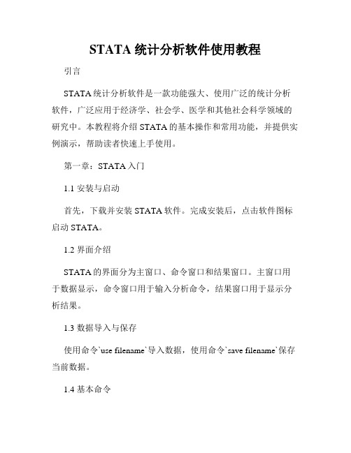
STATA统计分析软件使用教程引言STATA统计分析软件是一款功能强大、使用广泛的统计分析软件，广泛应用于经济学、社会学、医学和其他社会科学领域的研究中。

本教程将介绍STATA的基本操作和常用功能，并提供实例演示，帮助读者快速上手使用。

第一章：STATA入门1.1 安装与启动首先，下载并安装STATA软件。

完成安装后，点击软件图标启动STATA。

1.2 界面介绍STATA的界面分为主窗口、命令窗口和结果窗口。

主窗口用于数据显示，命令窗口用于输入分析命令，结果窗口用于显示分析结果。

1.3 数据导入与保存使用命令`use filename`导入数据，使用命令`save filename`保存当前数据。

1.4 基本命令介绍常用的基本命令，如`describe`用于显示数据的基本信息、`summarize`用于计算变量的统计描述等。

第二章：数据处理与变量管理2.1 数据选择与筛选通过命令`keep`和`drop`选择和删除数据的特定变量和观察值。

2.2 数据排序与重编码使用命令`sort`对数据进行排序，使用命令`recode`对变量进行重编码。

2.3 缺失值处理介绍如何检测和处理数据中的缺失值，包括使用命令`missing`和`recode`等。

第三章：数据分析3.1 描述性统计介绍如何使用STATA计算和展示数据的描述性统计量，如均值、标准差、最大值等。

3.2 统计检验介绍如何进行常见的统计检验，如t检验、方差分析、卡方检验等。

3.3 回归分析介绍如何进行回归分析，包括一元线性回归、多元线性回归和逻辑回归等。

3.4 生存分析介绍如何进行生存分析，包括Kaplan-Meier生存曲线和Cox比例风险模型等。

第四章：图形绘制与结果解释4.1 图形绘制基础介绍如何使用STATA进行常见的数据可视化，如散点图、柱状图、折线图等。

4.2 图形选项与高级绘图介绍如何通过调整图形选项和使用高级绘图命令，进一步美化和定制图形。

Stata软件使用指南说明书

18Learning more about StataWhere to go from hereYou now know plenty enough to use Stata.There is still much,much more to learn because Stata is a rich environment for doing statistical analysis and data management.What should you do to learn more?•Get an interesting dataset and play with Stata.e the menus and dialog system to experiment with commands.Notice what commandsshow up in the Results window.You willﬁnd that Stata’s simple and consistent commandsyntax will make the commands easy to read so that you will know what you have doneand easy to remember so that typing some commands will be faster than using menus.b.Play with graphs and the Graph Editor.•If you venture into the Command window,you willﬁnd that many things will go faster.You will alsoﬁnd that it is possible to make mistakes where you cannot understand why Stata is balking.a.Try help commandname or Help>Stata command...and entering the command name.b.Look at the command syntax and the examples in the helpﬁle,and compare themwith what you pare them closely:small typographical errors make commandsimpossible for Stata to parse.•Explore Stata by selecting Help>Search....You will uncover many statistical routines that could be of great use.•Look through the Combined subject table of contents in the Stata Index.•Read and work your way through the User’s Guide.It is designed to be read from cover to cover,and it contains most of the information you need to become an expert Stata user.It is well worth reading.If you are not this ambitious and instead prefer to sample the User’s Guide and the references,there is some advice later in this chapter for you.•Browse through the reference manuals to read about statistical methods you like to use,making use of the links to jump to other topics.The reference manuals are not meant to be read from cover to cover—they are meant to be referred to as you would an encyclopedia.You canﬁnd the datasets used in the examples in the manuals by selecting File>Example datasets...and then clicking on Stata18manual datasets.Doing so will enable you to work through the examples quickly.•Stata has much information,including answers to frequently asked questions(FAQ s),at https:///support/faqs/.•There are many useful links to Stata resources at https:///links/.Be sure to look at these materials because many outstanding resources about Stata are listed here.•Join Statalist,a forum devoted to discussion of Stata and statistics.•Read The Stata Blog:Not Elsewhere Classiﬁed at https:// to read articles written by people at Stata about all things Stata.•Visit Stata on Facebook at https:///statacorp,join Stata on Instagram at https:///statacorp,ﬁnd Stata on LinkedIn at https:///company/statacorp,and follow Stata on Twitter at https:///stata to keep up with Stata.•Subscribe to the Stata Journal,which contains reviewed papers,regular columns,book reviews, and other material of interest to researchers applying statistics in a variety of disciplines.Visit https://.12[GSM]18Learning more about Stata•Many supplementary books about Stata are available.Visit the Stata Bookstore athttps:///bookstore/.•Take a Stata NetCourse R .NetCourse101is an excellent choice for learning about Stata.See https:///netcourse/for course information and schedules.•Attend a classroom or a web-based training course taught by StataCorp.Visithttps:///training/classroom-and-web/for course information and schedules.•View a webinar led by Stata developers.Visit https:///training/webinar/for the current list of topics and schedule.•Watch Stata videos at https:///user/statacorp.Suggested reading from the User’s Guide and reference manuals The User’s Guide is designed to be read from cover to cover.The reference manuals are designed as references to be sampled when necessary.Ideally,after reading this Getting Started manual,you should read the User’s Guide from cover to cover,but you probably want to become at least somewhat proﬁcient in Stata right away.Here isa suggested reading list of sections from the User’s Guide and the reference manuals to help you onyour way to becoming a Stata expert.This list covers fundamental features and points you to some less obvious features that you might otherwise overlook.Basic elements of Stata[U]11Language syntax[U]12Data[U]13Functions and expressionsData management[U]6Managing memory[U]22Entering and importing data[D]import—Overview of importing data into Stata[D]append—Append datasets[D]merge—Merge datasets[D]compress—Compress data in memory[D]frames intro—Introduction to framesGraphics[G]Stata Graphics Reference ManualReproducible research[U]16Do-ﬁles[U]17Ado-ﬁles[U]13.5Accessing coefﬁcients and standard errors[U]13.6Accessing results from Stata commands[U]21Creating reports[RPT]Dynamic documents intro—Introduction to dynamic documents[RPT]putdocx intro—Introduction to generating Ofﬁce Open XML(.docx)ﬁles[RPT]putexcel—Export results to an Excelﬁle[RPT]putpdf intro—Introduction to generating PDFﬁles[R]log—Echo copy of session toﬁle[GSM]18Learning more about Stata3Useful features that you might overlook[U]29Using the Internet to keep up to date[U]19Immediate commands[U]24Working with strings[U]25Working with dates and times[U]26Working with categorical data and factor variables[U]27Overview of Stata estimation commands[U]20Estimation and postestimation commands[R]estimates—Save and manipulate estimation resultsBasic statistics[R]anova—Analysis of variance and covariance[R]ci—Conﬁdence intervals for means,proportions,and variances[R]correlate—Correlations of variables[D]egen—Extensions to generate[R]regress—Linear regression[R]predict—Obtain predictions,residuals,etc.,after estimation[R]regress postestimation—Postestimation tools for regress[R]test—Test linear hypotheses after estimation[R]summarize—Summary statistics[R]table intro—Introduction to tables of frequencies,summaries,and command results [R]tabulate oneway—One-way table of frequencies[R]tabulate twoway—Two-way table of frequencies[R]ttest—t tests(mean-comparison tests)Matrices[U]14Matrix expressions[U]18.5Scalars and matrices[M]Mata Reference ManualProgramming[U]16Do-ﬁles[U]17Ado-ﬁles[U]18Programming Stata[R]ml—Maximum likelihood estimation[P]Stata Programming Reference Manual[M]Mata Reference ManualSystem values[R]set—Overview of system parameters[P]creturn—Return c-class values4[GSM]18Learning more about StataInternet resourcesThe Stata website(https://)is a good place to get more information about Stata.You willﬁnd answers to FAQ s,ways to interact with other users,ofﬁcial Stata updates,and other useful information.You can also join Statalist,a forum devoted to discussion of Stata and statistics.You will alsoﬁnd information on Stata NetCourses R ,which are interactive courses offered over the Internet that vary in length from a few weeks to eight weeks.Stata also offers in-person and web-based training sessions,as well as webinars on Stata features.Visit https:///learn/ for more information.At the website is the Stata Bookstore,which contains books that we feel may be of interest to Stata users.Each book has a brief description written by a member of our technical staff explaining why we think this book may be of interest.We suggest that you take a quick look at the Stata website now.You can register your copy of Stata online and request a free subscription to the Stata News.Visit https:// for information on books,manuals,and journals published by Stata Press.The datasets used in examples in the Stata manuals are available from the Stata Press website.Also visit https:// to read about the Stata Journal,a quarterly publication containing articles about statistics,data analysis,teaching methods,and effective use of Stata’s language.Visit Stata’s ofﬁcial blog at https:// for news and advice related to the use of Stata.The articles appearing in the blog are individually signed and are written by the same people who develop,support,and sell Stata.The Stata Blog:Not Elsewhere Classiﬁed also has links to other blogs about Stata,written by Stata users around the world.Follow Stata on Facebook at https:///statacorp,Twitter at https:///stata, Instagram at https:///statacorp,and LinkedIn athttps:///company/statacorp.You may also follow Stata on Twitter athttps:///stata fr or https:///stata es.These are good ways to stay up-to-the-minute with the latest Stata information.Watch short example videos of using Stata on YouTube at https:///user/statacorp.See[GSM]19Updating and extending Stata—Internet functionality for details on accessing ofﬁcial Stata updates and free additions to Stata on the Stata website.[GSM]18Learning more about Stata5 Stata,Stata Press,and Mata are registered trademarks of StataCorp LLC.Stata andStata Press are registered trademarks with the World Intellectual Property Organization®of the United Nations.Other brand and product names are registered trademarks ortrademarks of their respective companies.Copyright c 1985–2023StataCorp LLC,College Station,TX,USA.All rights reserved.。

Stata数据分析软件用户指南说明书

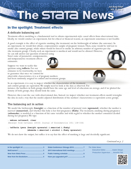
Jul/Aug/Sept Vol 30 No 3In the spotlight: Treatment effectsA delicate balancing actTreatment-effects modeling is a fundamental tool to obtain experimental-style causal effects from observational data. Ideally, we would conduct an experiment, but for ethical or financial reasons, an experiment sometimes is not feasible.A good example is the effect of cigarette smoking (the treatment) on the birthweight of infants (the outcome). Inan experiment, we would first obtain a representative sample of pregnant women. Then, some would be told not to smoke (the control group), while others would be forced to smoke an arbitrary number of cigarettes per day(the treatment group). Clearly, such an experiment is unethical and would not be allowed. However,we can still answer our question of interest usingStata’s suite of parametric, semiparametric,and nonparametric treatment-effectsestimators.Suppose we want to tackle thisquestion using teffects. For ourestimates to be trustworthy, we haveto guarantee that once we control forobservable characteristics, it is as if pregnant mothershad been randomly assigned to control and treatment groups.In an experiment, it is easy to inspect whether the characteristics of the treatmentand control groups are equivalent. We simply need to look at the data as observed. Forinstance, the mothers in both groups should have the same age and level of education on average, and if we plotted the density of both groups, they should look the same.However, this is not the case with observational data. Instead, we inspect whether our treatment-effects model reweights the data in such a way that the model-adjusted distribution of the mothers’ characteristics is equivalent across groups.The balancing act in actionWe model the birthweight (bweight) as a function of the number of prenatal visits (nprenatal), whether the mother is married (mmarried), and whether this baby is her first pregnancy (fbaby). The treatment, smoking during pregnancy (mbsmoke), is modeled as a function of the same variables and with regard to whether the mother consumed alcohol during her pregnancy. We type. webuse cattaneo2, clear(Excerpt from Cattaneo (2010) Journal of Econometrics 155: 138-154). teffects ipwra (bweight nprenatal i.mmarried i.fbaby)(mbsmoke i.mmarried i.alcohol i.fbaby nprenatal)We do not show the output, but suffice it to say that the effect of smoking is large and decidedly significant.Continued on p. 22The values in the Raw columns show that without controlling for covariates, the groups are very different. The values in the Weighted columns show the differences in means and the ratio of the variances of the control and treatment groups after reweighting for the covariates. The mean differences are all near zero, and the variance ratios are all close to one. These diagnostics suggest that after we control for the covariates, it is as if we had randomly assigned the mothers to either the control group or the treatment group.W e can also inspect this graphically by plotting the distribution before fitting our model and the distribution after weighting. W e do this for the number of prenatal visits. .tebalance density nprenatalThe density graphs confirm what we observe from our diagnostics.Can we do a test?What we have described so far is qualitative: we have diagnostics but not a formal test. We can, however, do a test. Intuitively, the score equations for the treatment and control groups should be the same. We can test whether this is the case by using the score equations as moments in an overidentification test. The null hypothesis is that our covariates are balanced. We type. tebalance overidOveridentification test for covariate balanceH0: Covariates are balanced:chi2(5) = 4.0425Prob > chi2 = 0.5433We cannot reject the null hypothesis. This impliesthat there is no evidence that our covariates remain imbalanced after reweighting.Parting wordsSometimes, we cannot conduct experiments, butwe can obtain experimental-style causal effects from observational data. For this to happen, we need to be able to say that our treatment-effects model reweights the data in such a way that the model-adjusted distribution ofthe covariates is equivalent across treatment groups. We can verify this with the postestimation diagnostic tests provided in teffects.—Enrique Pinzon Senior Econometrician, StataCorpT o obtain balancing diagnostics of the averages and variances of the mothers’ characteristics across groups, we type3 In the spotlight: irtNew to Stata 14 is a suite of commands to fit item response theory (IRT) models. IRT models are used to analyze the relationship between the latent trait of interest and the items intended to measure the trait. Stata’s irt commands provide easy access to some of the commonly used IRT models for binary and polytomous responses, and irtgraph commands can be used to plot characteristic functions and information functions.T o learn more about Stata’s IRT features, refer to the [IRT] Item Response Theory Reference Manual; here I want to go beyond the manual and show you some examples of what you can do with a little bit of Stata code.The dataset used in the examples contains answers to nine binary items, q1–q9. I do not show much Stata code here; see the accompanying blog entry at for details, including replication code.Example 1T o get started, I want to show you how simple IRT analysis is in Stata.When I use the nine binary items q1–q9, all I need to type to fit a 1PL model is. irt 1pl q*Equivalently, I can use a dash notation or explicitly spell out the variable names:. irt 1pl q1-q9. irt 1pl q1 q2 q3 q4 q5 q6 q7 q8 q9I can also use parenthetical notation:. irt (1pl q1-q9)Parenthetical notation is not very useful for a simple IRT model, but it comes in handy when you want to fit a single IRT model to combinations of binary, ordinal, and nominal items:. irt (1pl q1-q5) (1pl q6-q9) (pcm x1-x10) ...IRT graphs are equally simple to create in Stata. For example, to plot item characteristic curves (ICCs) for all the items in a model, I type. irtgraph iccY es, that’s it!Example 2Sometimes, I want to fit the same IRT model on two different groups and see how the estimated parameters differ between the groups. This exercise can be part of investigating differential item functioning (DIF) or parameter invariance.I split the data into two groups, fit two separate 2PL models, and create two scatterplots to see how close the parameter estimates for discrimination and difficulty are for the two groups. For simplicity, my group variable is 1 for odd-numbered observations and 0 for even-numbered observations.We see that the estimated parametersfor item q8 appear to differ betweenthe two groups.Example 3Continuing with the example above,I want to show you how to use alikelihood-ratio test to test for item-parameter differences between groups.4Using item q8 as an example, I want to fit one model that constrains item q8 parameters to be the same between the two groups and fit another model that allows these parameters to vary.The first model is easy. I can fit a 2PL model for the entire dataset, which implicitly constrains the parameters to be equal for both groups. I store the estimates under the name equal.. quietly irt 2pl q*. estimates store equalT o estimate the second model, I need the following:. irt (2pl q1-q7 q9) (2pl q8 if odd) (2pl q8 if !odd)Unfortunately, this is illegal syntax. I can, however, split the item into two new variables where each variable is restricted to the required subsample:. generate q8_1 = q8 if odd. generate q8_2 = q8 if !oddI estimate the second IRT model, this time with items q8_1 and q8_2 taking the place of the original q8:. quietly irt 2pl q1-q7 q8_1 q8_2 q9. estat report q8_1 q8_2Two-parameter logistic model Number of obs = 800Log likelihood = -4116.2064Coef. Std. Err. z P>|z| [95% Conf. Interval]q8_1Discrim | 1.095867 .2647727 4.14 0.000 .5769218 1.614812Diff -1.886126 .3491548 -5.40 0.000 -2.570457 -1.201795q8_2Discrim 1.93005 .4731355 4.08 0.000 1.002721 2.857378Diff -1.544908 .2011934 -7.68 0.000 -1.93924 -1.150577Now, I can perform the likelihood-ratio test:. lrtest equal ., forceLikelihood-ratio test LR chi2(2) = 4.53(Assumption: equal nested in .) Prob > chi2 = 0.1040The test suggests the first model is preferable even though the two ICCs clearly differ:SummaryIRT models are used to analyze the relationship betweenthe latent trait of interest and the items intended tomeasure the trait. Stata’s irt commands provide easyaccess to some of the commonly used IRT models, andirtgraph commands implement the most commonlyused IRT plots. With just a few extra steps, you can easilycreate customized graphs, such as the ones demonstratedabove, which incorporate information from separate IRTmodels. Don’t forget to see the accompanying blog entryat that shows the Stata code used in thisarticle.—Rafal RaciborskiSenior Statistical Developer, StataCorp5 NetCourses®New: Introduction toStatistical Graphics Using StataLearn how to communicate your data with Stata’spowerful graphics features. This course will introducedifferent kinds of graphs and demonstrate how to usethem for exploratory data analysis. T opics include howto use graphs to check model assumptions, how toformat, save, and export your graphs for publicationusing the Graph Editor, how to create custom graphschemes, how to create complex graphs by layering andcombining multiple graphs, how to use margins andmarginsplot, and more. The course also contains 94videos with detailed, step-by-step explanations of thedifferent graphs discussed in the course. Bonus materialincludes information on user-written graph commandsand useful data management tools.September 11–October 23, 2015 ......................$150.00Don’t forget our other NetCourses!Introduction to StataLearn how to use all of Stata’s tools and become a sophisticated Stata user. Y ou will understand the Stata environment, how to import and export data from different formats, how Stata’s intuitive syntax works, data management in Stata, and more.September 11–October 23, 2015 ........................$95.00 Introduction to Stata ProgrammingBecome an expert in organizing your work in Stata. Make the most of Stata’s scripting language to improve your workflow and create concretely reproducible analyses. Learn how to speed up your work and do more complete analyses.September 11–October 23, 2015 ......................$150.00 Advanced Stata ProgrammingLearn how to create and debug your own commands that are indistinguishable from the commands that ship with Stata. September 18–November 6, 2015 .....................$175.00Introduction to Univariate Time Series with StataLearn univariate time-series analysis with an emphasis on the practical aspects most needed by practitioners and applied researchers.September 18–November 6, 2015 .....................$295.00Introduction to Panel Data Using Stata Become an expert in the analysis and implementation oflinear, nonlinear, and dynamic panel-data estimators using Stata. Geared for researchers and practitioners in all fields, this course focuses on the interpretation of panel-data estimates and the assumptions underlying the models that give rise to them.September 25–November 6, 2015 .....................$295.00Introduction to Survival AnalysisUsing StataLearn how to effectively analyze survival data using Stata. We cover censoring, truncation, hazard rates, and survival functions. Discover how to set the survival-time characteristics of your dataset just once and apply any of Stata’s many estimators and statistics to those data. September 18–November 6, 2015 .....................$295.00Learn more and enroll:/netcourseThe dates above don’t work for you? No problem! NetCourseNow allows you to set the time and workat your own pace as well. It also gives you a personal NetCourse instructor to guide you through the course./netcourse/ncnow7CONFERENCE/chicago16#stata2016Keep up with future Stata Users Group meetings. We post our schedule at /meeting . Want to be notified when new meeting information is posted? Go to /alerts and sign up for an email alert today.2015 International Stata Users Group meetingsStockholm, Sweden September 4, /meeting/nordic-and-baltic15Canberra, Australia September 24–25, /meeting/australia15London, UKSeptember 10–11, 2015/meeting/uk15Madrid, SpainOctober 22, 2015/meeting/spain15Florence, Italy November 12–13, /meeting/italy15Lisbon, Portugal September 18, /meeting/portugal15Reaching new heightsJuly 28–29, 2016, at the Gleacher CenterCHICAGO20168Contact us979-696-4600 979-696-4601 (fax)***************** Please include your Stata serial number with all correspondence.Find a Stata distributor near you:/worldwideCopyright 2015 by StataCorp LP . Stata is a registered trademark of StataCorp LP .Public training scheduleUsing Stata Effectively: DataManagement, Analysis, and Graphics FundamentalsSeptember 22–23, 2015, Washington, DC October 13–14, 2015, Washington, DCAimed at both new Stata users and those who wish to learn techniques for efficient day-to-day use of Stata, this course enables you to use Stata in a reproducible manner, making collaborative changes and follow-up analyses much simpler. Exercises and Stata examples supplement the lessons.Survey Data Analysis Using StataOctober 15–16, 2015, Washington, DCSet up and analyze data from complex survey designs. The course covers the sampling methods used to collect survey data and how they affect the estimation of totals, ratios, and regression coefficients. The course also covers Stata’s support for many survey variance estimators,including linearization, balanced and repeated replications (BRR), and jackknife.Multilevel/Mixed Models Using Stata• Bayesian analysis• IRT (item response theory)• Unicode• Integration with Excel • More in treatment effects • Multilevel survival models • More in multilevel models• Denominator degrees of freedom • More in SEM• More in power and sample size • Markov-switching models • Panel-data survival models • Fractional outcome regression• Marginal means and marginal effects • Hurdle models。

1、下载文档前请自行甄别文档内容的完整性，平台不提供额外的编辑、内容补充、找答案等附加服务。
2、"仅部分预览"的文档,不可在线预览部分如存在完整性等问题,可反馈申请退款(可完整预览的文档不适用该条件!)。
3、如文档侵犯您的权益，请联系客服反馈,我们会尽快为您处理(人工客服工作时间：9:00-18:30)。

除了计量模型外，STATA的软件包中也可执行统计学中的估计和检定，甚至是多变量分析中的各项分析工具。

因此，STATA可以说是一个相当强而有力的统计软件。

一、安装STATA所须的内存容量不大，只有4.03MB。

此外，安装也相当简单，只要在〝SETUP〞上点两下，安装完成后再分别输入”Sn”、”Code”和”Key”即可开始使用。

但是安装过程中有一点必须注意的是，如下图所示，有”Intercooled”和”Small”两个选项。

一般而言，为了方便日后要设定较大的内存容量来处理大笔的资料，通常选择以”Intercooled”进行安装。

以此項進行安裝二、窗口介绍安装完成后，点选桌面上STATA的图标，窗口画面如下图所示。

为了使画面美观，我们可以将画面拉到自己喜欢的地方，如下图所示。

为了保存这个窗口画面，我们必须点选工具列上的”Prefs”下的”Save Windowing Preferences”。

如此一来，以后开启STATA时都会以此窗口画面呈现。

接下来，我们依序介绍四个窗口的功用：左上─Review：此一窗口用于记录在开启STATA后所执行过的所有指令。

此外，STATA还可以将执行过的指令储存下来，存在一个do-file内，下次即可再执行相同的指令。

左下─Variables：此一窗口用于呈现某笔数据中的所有变量。

换言之，当数据中的变量都有其名称时，变量名称将会出现在此一窗口中。

只要数据有读进STATA中，变量名称就会出现。

它的优点是(1)确认数据输入无误；(2)只要在某变量上点选两下，该变量即会出现在窗口”Stata Command”上。

右上─Stata Results：此一窗口用于呈现并记录指令执行后的结果。

右下─Stata Command：此一窗口用于输入所欲执行的指令。

Note：以上四个窗口都可以从”Fonts”去更改字体大小。

三、输入数据（Entering data）在本小节中，我们将介绍如何把数据读进STATA。

但是在正式介绍之前，我们必须先对几个一般性的指令（general command）有所了解，说明如下：cd：即change directory，简言之，告知STATA数据储存的地方。

例如当数据储存在e槽的sample数据夹时，则必须先输入cd e:\sample。

dir/ls：用来显示目录的内容。

set memory#m：设定内存的容量。

例如：当有一笔庞大的数据要处理时，则可设定100mb的容量，此时可输入set memory100m。

（输入指令memory可以知道内存容量的大小以及使用情况。

）set matsize#：设定所需的变量个数。

一般而言，不须对此部分进行设定，除非所欲处理的资料庞大或是当执行后出现matsize toosmall的讯息时再进行修改即可。

内建为40。

set more off/on：若欲执行结果以分页的型式呈现时，则输入set moreon；若欲执行结果同时呈现时，则输入set more off。

help：求助键。

后面必须接的是指令。

说明如何使用该指令，例如：help regress。

search：求助键。

后面可接任何文字。

说明在何处可以找到该文字。

例如：search normal distribution。

clear：清除键。

用来删除所有数据。

接下来，根据数据类型或指令的不同，数据输入的方法可分成以下四种：1、输入EXCEL数据将EXCEL的数据输入STATA的方式还可细分成以下两种：①将EXCEL的数据输入STATA之前，必须先将数据存成csv文件，再利用指令insheet来读数据。

Example：❶当csv档的第一列有变量名称时：❷当csv档的第一列没有变量名称时：②直接复制EXCEL上的数据，再到STATA选取”Window”下的”Data Editor”，点选后会出现”Stata Editor”工作表，再到”Edit”下选取”Paste”即可贴上数据。

2、输入ASCII的数据型态依ASCII的数据型态区分，将ASCII的数据输入STATA的方式也有以下两种：①数据型态一：见sample1-3.txtNote：记住文字的设定方式（str#variable name）。

②数据型态二：见sample1-4.txt第二种的数据型态通常须要codebook。

如下表所示。

3、利用Do-file editor输入数据将数据或是指令写入Do-file editor，再执行即可。

例如：将下面数据复制并贴在Do-file editor（选取”Window”下的”Do-file editor”）上，再选择”do currnet file”执行即可。

4、利用STATA的数据型态输入除了以上三种方法之外，还可以开启之前以STATA储存的资料。

Note：此一指令亦可用在读取网络上的数据（use网址）。

最后，将数据输入的相关指令整理成下表。

四、探索资料（Exploring data）为了更详细地呈现出在数据探索时所需使用的相关指令，我们利用sample4-1来说明指令的用法。

首先，利用前节所提及的数据输入方法将sample4-1读进STATA。

在正式分析数据之前，我们可以利用一个log档来储存之后所要执行的指令以及所得到的结果。

指令的表示方法如下：接下来，我们可以先利用下面的指令来检视sample4-1的数据：count：可得样本数。

describe：描述数据来源以及数据大小。

list：依序列出观察值的各个变量值。

codebook：描述资料的详细内容。

此外，我们就可以利用summarize、tabulate和tabstat等指令得到数据的叙述统计与基本特性。

表示如下：summarize：列出资料的叙述统计。

Example：summarize write,detailsum write if read>=60（sum是summarize的简写）sum write if prgtype=="academic"（接在if之后的句子中的”=”要放两个）sum write in1/40（只列出第1笔到第40笔资料）tabulate：列出变数的次数表。

Example：tabulate prgtypetabulate prgtype racetabulate prgtype,summarize(read)tabulate prgtype race,summarize(write)tabstat：列出变量的叙述统计。

Example：tabstat read write math,by(prgtype)stat(n mean sd)tabstat write,stat(n mean sd p25p50p75)by(prgtype)接下来，我们介绍一些用来划图的指令：茎叶图：stem writestem write,lines(2)直方图：graph write,bin(10)graph write,hist normal bin(10)箱形图：graph write,boxsort prgtype（要先有这个指令才能执行下一个指令）graph write,box by(prgtype)此外，利用correlate或是pwcorr可以得到相关矩阵；亦可利用graph 划出散布图。

现在我们可以将log文件结束了，指令输入如下：若欲检视log档中的结果，可以输入指令：或是到所储存的目录下点选。

最后，将数据探索的相关指令整理成下表。

五、修饰资料（Modifying data）在本小节中，我们亦利用sample4-1的数据进行说明。

首先，读进数据。

读完数据后，可以为此数据取个名称，指令如下：现在我们可以将变量的顺序作一排列。

例如：原先的变量顺序为gender、id和race…，但是我们想把顺序改成id、gender和race…，则可以下面的指令来执行：在执行codebook时，我们会发现有些变量尚未加上卷标（label），为了更清楚地表达变量所代表的意义，我们可以执行以下的指令：现在，我们想要产生一个新变量total，此变量代表read、write和math 的总和。

指令如下：此外，若是我们想加总的分数是read、write和socst，而非read、write和math，此时的指令输入如下：另一方面，我们还可以将变量total表示成以等级（A、B、C、D and F）的形式。

指令如下：为了记忆变量的意义为何，我们还可以利用note的方式来记录变量。

指令如下：另外，介绍一些利用公式来产生变量的指令。

最后，我们可以将以上的执行结果储存下来。

指令如下：现在亦将数据修饰的相关指令整理成下表。

六、管理数据（Managing data）在本节中，我们将进一步介绍如何将数据作一些特殊的处理，例如：保留所欲分析的数据、删除多余的数据或是将两份数据结合等等。

假设我们只想针对部分的数据进行处理，而又想保留原始资料时，则有以下两种方法可进行：1、另存新檔：亦即将所欲分析的部分数据储存在另一个档案中。

例如：我们只针对read成绩大于或是等于60分的学生进行分析，则可利用下面的指令来筛选。

Note：当只要保留某些变量时，则利用指令keep。

例如：keep read write。

2、直接处理：亦即在原始数据上进行分析。

承上例，指令输入如下：Note：若要删除某些变量时，则利用指令drop。

例如：drop read write。

接下来，我们介绍如何将两笔数据结合在一起。

数据的结合主要可以分为两种，水平合并和垂直合并。

前者是指变量的增加；后者则是指样本数的增加。

说明如下：1、水平合并2、垂直合并：Note：在垂直合并前要记得先sort。

最后，我们将数据修饰的相关指令整理成下表。

七、资料分析透过前面几节的介绍，应该对于STATA的指令和使用方法有了基本的认识。

现在，我们开始说明如何利用STATA来处现统计上的问题以及计量方面的模型。

1、检定：我们利用下面的例子来示范如何进行统计上的检定工作。

2、回归在执行回归分析时所使用的指令为regress。

另外，当存在heterogeneity of variance的问题时，可在后面加上robust；另外，若是不想放入截距项时，可在后面加上noconstant。

若欲得到残差值，可输入以下指令：123、二元选择模型在执行二元选择模型时所使用的程序写法与执行回归分析时相同，只是所使用的指令不同。