Percolation model for nodal domains of chaotic wave functions
FORNELL教授经典的顾客满意度论文1
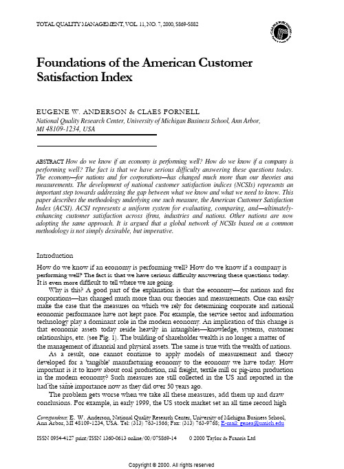
TOTAL QUALITY MANAGEMENT, VOL. 11, NO. 7, 2000, S869-S882EUGENE W. ANDERSON & CLAES FORNELLNational Quality Research Center, University of Michigan Business School, Ann Arbor,MI 48109-1234, USAABSTRACT How do we know if an economy is performing well? How do we know if a company is performing well? The fact is that we have serious difficulty answering these questions today. The economy—for nations and for corporations—has changed much more than our theories and measurements. The development of national customer satisfaction indices (NCSIs) represents an important step towards addressing the gap between what we know and what we need to know. This paper describes the methodology underlying one such measure, the American Customer Satisfaction Index (ACSI). ACSI represents a uniform system for evaluating, comparing, and—ultimately- enhancing customer satisfaction across ifrms, industries and nations. Other nations are now adopting the same approach. It is argued that a global network of NCSIs based on a common methodology is not simply desirable, but imperative.IntroductionHow do we know if an economy is performing well? How do we know if a company is performing well? The fact is that we have serious difficulty answering these questions today. It is even more difficult to tell where we are going.Why is this? A good part of the explanation is that the economy—for nations and for corporations—has changed much more than our theories and measurements. One can easily make the case that the measures on which we rely for determining corporate and national economic performance have not kept pace. For example, the service sector and information technology play a dominant role in the modern economy. An implication of this change is that economic assets today reside heavily in intangibles—knowledge, systems, customer relationships, etc. (see Fig. 1). The building of shareholder wealth is no longer a matter of the management of ifnancial and physical assets. The same is true with the wealth of nations.As a result, one cannot continue to apply models of measurement and theory developed for a 'tangible' manufacturing economy to the economy we have today. How important is it to know about coal production, rail freight, textile mill or pig-iron production in the modern economy? Such measures are still collected in the US and reported in the media as if theyhad the same importance now as they did over 50 years ago.The problem gets worse when we take all these measures, add them up and draw conclusions. For example, in early 1999, the US stock market set an all time record highCorrespondence: E. W. Anderson, National Quality Research Center, University of Michigan Business School, Ann Arbor, MI 48109-1234, USA. Tel: (313) 763-1566; Fax: (313) 763-9768; E-mail: genea@ISSN 0954-4127 print/ISSN 1360-0613 online/00/07S869-14 0 2000 Taylor & Francis LtdS870 E. W. ANDERSON & C. FORNELLDow Jones Industrials:Price-to-Book Ratios11970 1999Source: Business Week, March 9, 1999Figure 1. Tangible versus intangible sources of value, 1970-99.with the Dow Jones Index passing 11 000 points, unemployment was at record lows, the economy expanded and inflation was almost non-existent. These statistics suggested a strong economy, which was also what was reported in the press and in most commentary by economists. As always, however, the real question is: Are we better off? How well are the actual experiences of people captured by the reported measures? Do the things economists and Governments choose to measure correspond with how people feel about their economic well-being? A closer inspection of the numbers and their underlying statistics reveals a somewhat different picture of the US economy than that typically held up as an example.?Corporate earnings growth for 1997 and 1998 were much lower than in the previous2 years, with a negative growth for 1998.?The major portion of the earnings growth in 1995 and 1996 was due to cost-cutting rather than revenue growth.?The trade deficit in 1999 was at a record high and growing.?Wages have been stagnant in the last 15 years (although there were small increases in 1997 and 1998).?The proportion of stock market capitalization versus GDP was about 150% of GDP in 1998 (the historical average is 48%; the proportion before the 1929 stock market crash was 82%).?Consumer and business debt were high and rising.?Even though many new jobs were created, 70% of those who lost their jobs got new jobs that paid less.?The number of bankruptcies was high and growing.?Worker absenteeism was at record highs.?Household savings were negative.Add the above to the fact that there is a great deal of worker anxiety over job security and lower levels of customer satisfaction than 5 years ago, and the question of whether we areyrFOUNDATIONS OF ACSI S871better off is cast in a different light. How much does it matter if we increase productivity,that the economy is growing or that the stock market is breaking records, if customers arenot satisifed? The basic idea behind a market economy is that businesses exist and competein order to create a satisifed customer. Investors will lfock to the companies that are expectedto do this well. It is not possible to increase economic prosperity without also increasingcustomer satisfaction. In a market economy, where suppliers compete for buyers, but buyersdo not compete for products, customer satisfaction defines the meaning of economic activity,because what matters in the final analysis is not how much we produce or consume, but howwell our economy satisfies its consumers.Together with other economic objectives—such as employment and growth—thequality of what is produced is a part of standard of living and a source of national competitiveness. Like other objectives, it should be subjected to systematic and uniform measurement. This is why there is a need for national indices of customer satisfaction. Anational index of customer satisfaction contributes to a more accurate picture of economicoutput, which in turn leads to better economic policy decisions and improvement of standard ofliving. Neither productivitymeasures nor price indices can be properly calibrated without taking quality into account.It is difficult to conduct economic policy without accurate and comprehensive measures. Customer satisfaction is of considerable value as a complement to the traditional measures.This is true for both macro and micro levels. Because it is derived from consumption data(as opposed to production) it is also a leading indicator of future proifts. Customer satisfactionleads to greater customer loyalty (Anderson & Sullivan, 1993; Bearden & Teel, 1983; Bolton& Drew, 1991; Boulding et al., 1993; Fornell, 1992; LaBarbera & Mazurski, 1983; Oliver,1980; Oliver & Swan, 1989; Yi, 1991). Through increasing loyalty, customer satisfactionsecures future revenues (Bolton, 1998; Fornell, 1992; Rust et al., 1994, 1995), reduces thecost of future transactions (Reichheld & Sasser, 1990), decreases price elasticities (Anderson,1996), and minimizes the likelihood customers will defect if quality falters (Anderson & Sullivan, 1993). Word-of-mouth from satisifed customers lowers the cost of attracting new customers and enhances the firm's overall reputation, while that of dissatisifed customersnaturally has the opposite effect (Anderson, 1998; Fornell, 1992). For all these reasons, it isnot surprising that empirical work indicates that ifrms providing superior quality enjoy higher economic returns (Aaker & Jacobson, 1994; Anderson et al., 1994, 1997; Bolton, 1998;Capon et al., 1990).Satisfied customers can therefore be considered an asset to the ifrm and should be acknowledged as such on the balance sheet. Current accounting-based measures are probablymore lagging than leading—they say more about past decisions than they do about tomorrow's performance (Kaplan & Norton, 1992). If corporations did incorporate customer satisfactionas a measurable asset, we would have a better accounting of the relationship between theenterprise's current condition and its future capacity to produce wealth.If customer satisfaction is so important, how should it be measured? It is too complicatedand too important to be casually implemented via standard market research surveys. The remainder of this article describes the methodology underlying the American Customer Satisfaction Index (ACSI) and discusses many of the key ifndings from this approach.Nature of the American Customer Satisfaction IndexACSI measures the quality of goods and services as experienced by those that consume them.An individual ifrm's customer satisfaction index (CSI) represents its served market's—its customers'—overall evaluation of total purchase and consumption experience, both actualand anticipated (Anderson et al., 1994; Fonrell, 1992; Johnson & Fornell, 1991).S872 E. W. ANDERSON & C. FORNELLThe basic premise of ACSI, a measure of overall customer satisfaction that is uniform and comparable, requires a methodology with two fundamental properties. (For a complete description of the ACSI methodology, please see the 'American Customer Staisfaction Index: Methodology Report' available from the American Society for Quailty Control, Milwaukee, WI.) First, the methodology must recognize that CSI is a customer evaluation that cannot be measured directly. Second, as an overall measure of customer satisfaction, CSI must be measured in a way that not only accounts for consumption experience, but is also forward-looking.Direct measurement of customer satisfaction: observability with errorEconomists have long expressed reservations about whether an individual's satisfaction or utility can be measured, compared, or aggregated (Hicks, 1934, 1939a,b, 1941; Pareto, 1906; Ricardo, 1817; Samuelson, 1947). Early economists who believed it was possible to produce a 'cardinal' measure of utility (Bentham, 1802; Marshall, 1890; Pigou, 1920) have been replaced by ordinalist economists who argue that the structure and implications of utility-maximizing economics can be retained while relaxing the cardinal assumption. How_ ever, cardinal or direct measurement of such judgements and evaluations is common in other social sciences. For example, in marketing, conjoint analysis is used to measure individual utilities (Green & Srinivasan, 1978, 1990; Green & Tull, 1975).Based on what Kenneth Boulding (1972) referred to as Katona's Law (the summation of ignorance can produce knowledge due to the self-canceling of random factors), the recent advances in latent variable modeling and the call from economists such as the late Jan Tinbergen (1991) for economic science to address better what is required for economic policy, scholars are once again focusing on the measurement of subjective (experience) utility. The challenge is not to arrive at a measurement system according to a universal system of axioms, but rather one where fallibility is recognized and error is admitted (Johnson & Fornell, 1991) .The ACSI draws upon considerable advances in measurement technology over the past 75 years. In the 1950s, formalized systems for prediction and explanation (in terms of accounting for variation around the mean of a variable) started to appear. Before then, research was essentially descriptive, although the single correlation was used to depict the degree of a relationship between two variables. Unfortunately, the correlation coefficient was otfen (and still is) misinterpreted and used to infer much more than what is permissible. Even though it provides very little information about the nature of a relationship (any given value of the correlation coefficient is consistent with an inifnite number of linear relationships), it was sometimes inferred as having both predictive and causal properties. The latter was not achieved until the 1980s with the advent of the second generation of multivariate analysisand associated sotfware (e.g. Lisrel).It was not until very recently, however, that causal networks could be applied to customer satisfaction data. What makes customer satisfaction data difficult to analyze via traditional methods is that they are associated with two aspects that play havoc with most statistical estimation techniques: (1) distributional skewness; and (2) multicollinearity. Both are extreme in this type of data. Fortunately, there has been methodological progress on both fronts particularly from the field of chemometrics, where the focus has been on robust estimation with small sample sizes and many variables.Not only is it now feasible to measure that which cannot be observed, it is also possible to incorporate these unobservables into systems of equations. The implication is that the conventional argument for limiting measurement to that which is numerical is no longer allFOUNDATIONS OF ACSI S873that compelling. Likewise, simply because consumer choice, as opposed to experience, is publicly observable does not mean that it must be the sole basis for utility measurement. Such reasoning only diminishes the influence of economic science in economic policy (Tinbergen 1991).Hence, even though experience may be a private matter, it does not follow that it is inaccessible to measurement or irrelevant for scientific inquiry, for cardinalist comparisons of utility are not mandatory for meaningful interpretation. For something to be 'meaningful,' it does not have to be 'flawless' or free of error. Even though (experience) utility or customer satisfaction cannot be directly observed, it is possible to employ proxies (fallible indicators) to capture empirically the construct. In the ifnal analysis, success or failure will depend on how well we explain and predict.Forward-looking measurement of customer satisfaction: explanation and predictionFor ACSI to be forward-looking, it must be embedded in a system of cause-and-effect relationships as shown in Fig. 2, making CSI the centerpiece in a chain of relationships running from the antecedents of customer satisfaction —expectations, perceived quality and value —to its consequences —voice and loyalty. The primary objective in estimating this system or model is to explain customer loyalty. It is through this design that ACSI captures the served market's evaluation of the ifrm's offering in a manner that is both backward- and forward-looking.Customer satisfaction (ACSI) has three antecedents: perceived quality, perceived value and customer expectations. Perceived quality or performance, the served market's evaluation of recent consumption experience, is expected to have a direct and positive effect on customer satisfaction. The second determinant of customer satisfaction is perceived value, or the perceived level of product quality relative to the price paid. Adding perceived value incorpo-rates price information into the model and increases the comparability of the results across ifrms, industries and sectors. The third determinant, the served market's expectations, represents both the served market's prior consumption experience with the firm's offeringCustomization Complaints to Complaints toinagement PersonnelPriceü GivenQualityQualityGivenPrice DelepurchasePrice Likelihood ToleranceCustomization Reliability O v e r a l l Figure 2. The American Customer Satisfaction Index model.S874 E. W. ANDERSON & C. FORNELLincluding non-experiential information available through sources such as advertising and word-of-mouth—and a forecast of the supplier's ability to deliver quality in the future.Following Hirschman's (1970) exit-voice theory, the immediate consequences of increased customer satisfaction are decreased customer complaints and increased customer loyalty (Fornell & Wemerfelt, 1988). When dissatisifed, customers have the option of exiting (e.g. going to a competitor) or voicing their complaints. An increase in satisfaction should decrease the incidence of complaints. Increased satisfaction should also increase customer loyalty. Loyalty is the ultimate dependent variable in the model because of its value as aproxy for profitability (Reichheld & Sasser, 1990).ACSI and the other constructs are latent variables that cannot be measured directly, each is assessed by multiple measures, as indicated in Fig. 1. To estimate the model requires data from recent customers on each of these 15 manifest variables (for an extended discussion of the survey design, see Fomell et al., 1996). Based on the survey data, ACSI is estimated as shown in Appendix B.Customer satisfaction index properties: the case of the American Customer Satisfaction IndexAt the most basic level the ACSI uses the only direct way to ifnd out how satisifed or dissatisifed customers are—that is, to ask them. Customers are asked to evaluate products and services that they have purchased and used. A straightforward summary of what customers say in their responses to the questions may have certain simplistic appeal, but such an approach will fall short on any other criterion. For the index to be useful, it must meet criteria related to its objectives. If the ACSI is to contribute to more accurate and comprehen-sive measurement of economic output, predict economic returns, provide useful information for economic policy and become an indicator of economic health, it must satisfy certain properties in measurement. These are: precision; validity; reliability; predictive power; coverage; simplicity; diagnostics; and comparability.PrecisionPrecision refers to the degree of certainty of the estimated value of the ACSI. ACSI results show that the 90% confidence interval (on a 0-100 scale) for the national index is ± 0.2 points throughout its first 4 years of measurement. For each of the six measured private sectors, it is an average ± 0.5 points and for the public administration/government sector, it is + 1.3 points. For industries, the conifdence interval is an average ±1.0 points for manufacturing industries, + 1.7 points for service industries and ± 2.5 points for government agencies. For the typical company, it is an average ± 2.0 points for manufacturing ifrms and 2.6 points for service companies and agencies. This level of precision is obtained as a result of great care in data collection, careful variable speciifcation and latent variable modeling. Latent variable modeling produces an average improvement of 22% in precision over use of responses from a single question, according to ACSI research.ValidityValidity refers to the ability of the individual measures to represent the underlying construct customer satisfaction (ACSI) and to relate effects and consequences in an expected manner. Discriminant validity, which is the degree to which a measured construct differs from other measured constructs, is also evidenced. For example, there is not only an importanto-FOUNDATIONS OF ACSI S875 conceptual distinction between perceived quality and customer satisfaction, but also anempirical distinction. That is, the covariance between the questions measuring the ACSI ishigher than the covariances between the ACSI and any other construct in the system.The nomological validity of the ACSI model can be checked by two measures: (1) latentvariable covariance explained; and (2) multiple correlations (R'). On average, 94% of thelatent variable covariance structure is explained by the structural model. The average R2ofthe customer satisfaction equation in the model is 0.75. In addition, all coefficients relatingthe variables of the model have the expected sign. All but a few are statistically signiifcant.In measures of customer satisfaction, there are several threats to validity. The most seriousof these is the skewness of the frequency distributions. Customers tend disproportionately touse the high scores on a scale to express satisfaction. Skewness is addressed by using a fairlyhigh number of scale categories (1-10) and by using a multiple indicator approach (Fornell,1992, 1995). It is a well established fact that vaildity typically increases with the use of more categories (Andrews, 1984), and it is particularly so when the respondent has good knowledgeabout the subject matter and when the distribution of responses is highly skewed. An indexof satisfaction is much to be preferred over a categorization of respondents as either 'satisfied'or 'dissatisfied'. Satisfaction is a matter of degree—it is not a binary concept. If measured asbinary, precision is low, validity is suspect and predictive power is poor.ReliabilityReliability of a measure is determined by its signal-to-noise ratio. That is, the extent to whichthe variation of the measure is due to the 'true' underlying phenomenon versus randomeffects. High reliability is evident if a measure is stable over time or equivalent with identicalmeasures (Fonrell, 1992). Signal-to-noise in the items that make up the index (in terms of variances) is about 4 to 1.Predictive power and financial implications of ACSIAn important part of the ACSI is its ability to predict economic returns. The model, ofwhich the ACSI is a part, uses two proxies for economic returns as criterion variables: (1)customer retention (estimated from a non-linear transformation of a measure of repurchase likelihood); and (2) price tolerance (reservation price). The items included in the index areweighted in such a way that the proxies and the ACSI are maximally correlated (subject tocertain constraints). Unless such weighting is done, the index is more likely to include mattersthat may be satisfying to the customer, but for which he or she is not willing to pay.The empirical evidence for predictive power is available from both the Swedish data andthe ACSI data. Using data from the Swedish Barometer, a one-point increase in the SCSBeach year over 5 years yields, on the average, a 6.6% increase in current return-on-investment (Anderson et al., 1994). Of the firms traded on the Stockholm Stock Market Exchange, it isalso evident that changes in the SCSB have been predictive of stock returns.A basic tenet underlying the ACSI is that satisifed customers represent a real, albeit intangible, economic asset to a ifrm. By deifnition, an economic asset generates future incomestreams to the owner of that asset. Therefore, if customer satisfaction is indeed an economicasset, it should be possible to use the ACSI for prediction of company ifnancial results. It is,of course, of considerable importance that the ifnancial consequences of the ACSI arespecified and documented. If it can be shown that the ACSI is related to ifnancial returns,then the index demonstrates external validity.The University of Michigan Business School faculty have done considerable research onS876 E. W. ANDERSON & C. FORNELLthe linkage between ACSI and economic returns, analyzing both accounting and stock market returns from measured companies. The pattern from all of these studies suggests a statistically strong and positive relationship. Speciifcally:?There is a positive and significant relationship between ACSI and accounting return_ on-assets (Fornell et al., 1995).?There is a positive and signiifcant relationship between the ACSI and the market valueof common equity (Ittner & Larcker, 1996). When controlling for accounting book values of total assets and liabilities, a one-unit change (on the 0-100-point scale used for the ACSI) is associated with an average of US$646 million increase in market value. There are also significant and positive relationships between ACSI and market-to-book values and price/earnings ratios. There is a negative relationship between ACSI and risk measures, implying that firms with high loyalty and customersatisfactionhave less variability and stronger financial positions.?There is a positive and significant relationship between the ACSI and the long-term adjusted financial performance of companies. Tobin's Q is generally accepted as the best measure of long-term performance. It is deifned as the ratio of a firm's present value of expected cash lfows to the replacement costs of its assets. Controlling for other factors, ACSI has a significant relationship to Tobin's Q (Mazvancheryl et al.,1999).?Since 1994, changes in the ACSI have correlated with the stock market (Martin,1998). The current market value of any security is the market's estimate of the discounted present value of the future income stream that the underlying asset will generate. If the most important asset is the satisfaction of the customer base, changes in ACSI should be related to changes in stock price. Until 1997, the stock market went up, whereas ACSI went down. However, in quarters following a sharp drop in ACSI, the stock market has slowed. Conversely, when the ACSI has gone down only slightly, the following quarter's stock market has gone up substantially. For the 6 years of ACSI measurement, the correlation between changes in the ACSI and changes in the Dow Jones industrial average has been quite strong. The interpretation of this relationship suggests that stock prices have responded to downsizing, cost cutting and productivity improvements, and that the deterioration in quality (particularly in the service sectors) has not been large enough to offset the positive effects. It also suggests that there is a limit beyond which it is unlikely that customers will tolerate further decreases in satisfaction. Once that limit is reached (which is now estimated to be approximately —1.4% quarterly decline in ACSI), the stock market will not go up further.ACSI scores of approximately 130 publicly traded companies display a statistically positive relationship with the traditional performance measures used by firms and security analysts (i.e. return-on-assets, return-on-equity, price—earnings ratio and the market-to-book ratio). In addition, the companies with the higher ACSI scores display stock price returns above the market adjusted average (Ittner & Larcker, 1996). The ACSI is also positively correlated with 'market value added'. This evidence indicates that the ACSI methodology produces a reliable and valid measure for customer satisfaction that is forward-looking and relevant to a company's economic performance.CoverageThe ACSI measures a substantial portion of the US economy. In terms of sales dollars, it is approximately 30% of the GDP. The measured companies produce over 40%, but the ACSIFOUNDATIONS OF ACSI S877measures only the sales of these companies to household consumers in the domestic market. The economic sectors and industries covered are discussed in Chapter III. Within each industry, the number of companies measured varies from 2 to 22.The national index and the indices for each industry and sector are relfective of the total value (quality times sales) of products and services provided by the ifrms at each respective level of aggregation. Relative sales are used to determine each company's or agency's contribution to its respective industry index. In turn, relative sales by each industry are used to determine each industry's contribution to its respective sector index. To calculate the national index, the percentage contributions of each sector to the GDP are used to top-weight the sector indices. Mathematically, this is deifned as:Index for industry i in sector s at time t = ES f i;If _S S ,, S I Index for sector s at time t =I g = E ,whereSr…, = sales by ifrm f, industry i, sector s at time t= index for firm f, industry i, sector s at time tandSit = E S,, = total sales for industry i at time tS, = E S i , = total sales for sector s at time t ,The index is updated on a quarterly basis. For each quarter, new indices are estimated for one or two sectors with total replacement of all data annually at the end of the third calendar quarter. The national index is comprised of the most recent estimate for each sectorT S National index at time t — ____________ E 4, V s9t t =T -3 s W,13where I s , = 0 for all t in which the index for a sector is not estimated, and I = I for all ,, quarters in which an index is estimated. In this way, the national index represents company, industry and sector indices for the prior year.SimplicityGiven the complexity of model estimation, the ACSI maintains reasonable simpilcity. It is calibrated on a 0-100 scale. Whereas the absolute values of the ACSI are of interest, much of the index's value, as with most other economic indicators, is found in changes over time, which can be expressed as percentages.DiagnosticsThe ACSI methodology estimates the relationships between customer satisfaction and its causes as seen by the customer: customer expectations, perceived quality and perceived value. Also estimated are the relationships between the ACSI, customer loyalty (as measured by customer retention and price tolerance (reservation prices)) and customer complaints. The。
AIC信息准则

G: collection of “admissible” models (in terms of probability density functions). ˆ θ is MLE estimate based on model g and data y. y is the random sample from the density function f (x). • Model Selection Criterion ˆ Maximizing Ey Ex[log(g(x|θ(y)))]
Ω
f (x) log
f (x) dx g(x|θ) f (x) log(g(x|θ))dx
Ω
=
Ω
f (x) log(f (x))dx −
relative K-L information f : full reality or truth in terms of a probability distribution. g: approximating model in terms of a probability distribution. θ: parameter vector in the approximating model g. • Remark I(f, g) ≥ 0, with I(f, g) = 0 if and only if f = g almost everywhere. I(f, g) = I(g, f ), which implies K-L information is not the real “distance”.
March 15, 2007
-2-
background
Estimation error variance bias parameter vector for the full reality model. is the projection of ϑ onto the parameter space of the approximating model Θk . the maximum likelihood estimate of θ in Θk . Variance ˆ For sufficiently large sample size n, we have n θ − θ
J. Comput. Chem.
2D Depiction of Nonbonding Interactions forProtein ComplexesPENG ZHOU,1FEIFEI TIAN,2ZHICAI SHANG11Institute of Molecular Design&Molecular Thermodynamics,Department of Chemistry,Zhejiang University,Hangzhou310027,China2College of Bioengineering,Chongqing University,Chongqing400044,ChinaReceived7May2008;Revised25June2008;Accepted22July2008DOI10.1002/jcc.21109Published online22October2008in Wiley InterScience().Abstract:A program called the2D-GraLab is described for automatically generating schematic representation of nonbonding interactions across the protein binding interfaces.The inputfile of this program takes the standard PDB format,and the outputs are two-dimensional PostScript diagrams giving intuitive and informative description of the protein–protein interactions and their energetics properties,including hydrogen bond,salt bridge,van der Waals interaction,hydrophobic contact,p–p stacking,disulfide bond,desolvation effect,and loss of conformational en-tropy.To ensure these interaction information are determined accurately and reliably,methods and standalone pro-grams employed in the2D-GraLab are all widely used in the chemistry and biology community.The generated dia-grams allow intuitive visualization of the interaction mode and binding specificity between two subunits in protein complexes,and by providing information on nonbonding energetics and geometric characteristics,the program offers the possibility of comparing different protein binding profiles in a detailed,objective,and quantitative manner.We expect that this2D molecular graphics tool could be useful for the experimentalists and theoreticians interested in protein structure and protein engineering.q2008Wiley Periodicals,Inc.J Comput Chem30:940–951,2009Key words:protein–protein interaction;nonbonding energetics;molecular graphics;PostScript;2D-GraLabIntroductionProtein–protein recognition and association play crucial roles in signal transduction and many other key biological processes. Although numerous studies have addressed protein–protein inter-actions(PPIs),the principles governing PPIs are not fully under-stood.1,2The ready availability of structural data for protein complexes,both from experimental determination,such as by X-ray crystallography,and by theoretical modeling,such as protein docking,has made it necessary tofind ways to easily interpret the results.For that,molecular graphics tools are usually employed to serve this purpose.3Although a large number of software packages are available for visualizing the three-dimen-sional(3D)structures(e.g.PyMOL,4GRASP,5VMD,6etc.)and interaction modes(e.g.MolSurfer,7ProSAT,8PIPSA,9etc.)of biomolecules,the options for producing the schematic two-dimensional(2D)representation of nonbonding interactions for PPIs are very scarce.Nevertheless,a few2D graphics programs were developed to depict protein-small ligand interactions(e.g., LIGPLOT,10PoseView,11MOE,12etc.).These tools,however, are incapable of handling the macromolecular complexes.Some other available tools presenting macromolecular interactions in 2D level mainly include DIMPLOT,10NUCPLOT,13and MON-STER,14etc.Amongst,only the DIMPLOT can be used for aesthetically visualizing the nonbinding interactions of PPIs. However,such a program merely provides a simple description of hydrogen bonds,hydrophobic interactions,and steric clashes across the binding interfaces.In this article,we describe a new molecular graphics tool, called the two-dimensional graphics lab for biosystem interac-tions(2D-GraLab),which adopts the page description language (PDL)to intuitively,exactly,and detailedly reproduce the non-bonding interactions and energetics properties of PPIs in Post-Script page.Here,the following three points are the emphasis of the2D-GraLab:(i)Reliability.To ensure the reliability,the pro-grams and methods employed in2D-GraLab are all widely used in chemistry and biology community;(ii)Comprehensiveness. 2D-GraLab is capable of handling almost all the nonbonding interactions(and even covalent interactions)across binding Additional Supporting Information may be found in the online version of this article.Correspondence to:Z.Shang;e-mail:shangzc@interface of protein complexes,such as hydrogen bond,salt bridge,van der Waals(vdW)interaction,hydrophobic contact, p–p stacking,disulfide bond,desolvation effect,and loss of con-formational entropy.The outputted diagrams are diversiform, including individual schematic diagram and summarized sche-matic diagram;(iii)Artistry.We elaborately scheme the layout, color match,and page style for different diagrams,with the goal of producing aesthetically pleasing2D images of PPIs.In addi-tion,2D-GraLab provides a graphical user interface(GUI), which allows users to interact with this program and displays the spatial structure and interfacial feature of protein complexes (see .Fig.S1).Identifying Protein Binding InterfacesAn essential step in understanding the molecular basis of PPIs is the accurate identification of interprotein contacts,and based upon that,subsequent works are performed for analysis and lay-out of nonbonding mon methods identifyingprotein–protein binding interfaces include a Voronoi polyhedra-based approach,changes in solvent accessible surface area(D SASA),and various radial cutoffs(e.g.,closest atom,C b,andcentroid,etc.).152D-GraLab allows for the identification of pro-tein–protein binding interfaces at residue and atom levels.Identifying Binding Interfaces at Residue LevelAll the identifying interface methods at residue level belong toradial cutoff approach.In the radial cutoff approach,referencepoint is defined in advance for each residue,and the residues areconsidered in contact if their reference points fell within thedefined cutoff ually,the C a,C b,or centroid are usedas reference point.16–18In2D-GraLab,cutoff distance is moreflexible:cutoff distance5r A1r B1d,where r A and r B are residue radii and d is set by users(as the default d54A˚,which was suggested by Cootes et al.19).Identifying Binding Interfaces at Atom LevelAt atom level,binding interfaces are identified using closestatom-based radial cutoff approach20and D SASA-basedapproach.21For the closest atom-based radial cutoff approach,ifthe distance between any two atoms of two residues from differ-ent chains is less than a cutoff value,the residues are consideredin contact;In the D SASA-based approach,the SASA is calcu-lated twice to identify residues involved in a binding interface,once for the monomers and once for the complex,if there is achange in the SASA(D SASA)of a residue when going from themonomers to the dimer form,then it is considered involved inthe binding interface.In2D-GraLab,three manners are provided for visualizing thebinding interfaces,including spatial structure exhibition,residuedistance plot,and residue-pair contact map(see .Figs.S2–S4).Analysis and2D Layout of NonbondingInteractionsThe inputfile of2D-GraLab is standard PDB format,and the outputs are two-dimensional PostScriptfile giving intuitive and informative representation of the PPIs and their strengths, including hydrogen bond,salt bridge,vdW interaction,desolva-tion effect,ion-pair,side-chain conformational entropy(SCE), etc.The outputs are in two forms as individual schematic dia-gram and summarized schematic diagram.The individual sche-matic diagram is a detailed depiction of each nonbonding profile,whereas the summarized schematic diagram covers all nonbonding interactions and disulfide bonds across the binding interface.To produce the aesthetically high quality layouts,which pos-sess reliable and accurate parameters,several widely used pro-grams listed in Table1are employed in2D-GraLab to perform the core calculations and analysis of different nonbonding inter-actions.2D-GraLab carries out prechecking procedure for pro-tein structures and warns the structural errors,but not providing revision and refinement functions.Therefore,prior to2D-GraLab analysis,protein structures are strongly suggested to be prepro-cessed by programs such as PROCHECK(structure valida-tion),27Scwrl3(side-chain repair),28and X-PLOR(structure refinement).29Individual Schematic DiagramHydrogen BondThe program we use for analyzing hydrogen bonds across bind-ing interfaces is HBplus,23which calculates all possible posi-tions for hydrogen atoms attached to donor atoms which satisfy specified geometrical criteria with acceptor atoms in the vicinity. In2D-GraLab,users can freely select desired hydrogen bonds involving N,O,and/or S atoms.Besides,the water-mediated hydrogen bond is also given consideration.Bond strength of conventional hydrogen bonds(except those of water-mediated Table1.Standalone Programs Employed in2D-GraLab.Program FunctionReduce v3.0322Adding hydrogen atoms for proteinsHBplus v3.1523Identifying hydrogen bonds and calculatingtheir geometric parametersProbe v2.1224Identifying steric contacts and clashes at atomlevelMSMS v2.6125Calculating SASA values of protein atoms andresiduesDelphi v4.026Calculating Coulombic energy and reactionfield energy,determining electrostatic energyof ion-pairsDIMPLOT v4.110Providing application programming interface,users can directly set and executeDIMPLOT in the2D-GraLab GUI9412D Depiction of Nonbonding Interactions for Protein ComplexesFigure1.(a)Schematic representation of a conventional hydrogen bond and a water-mediated hydro-gen bond across the binding interface of IGFBP/IGF complex(PDB entry:2dsr).This diagram was produced using2D-Gralab.The conventional hydrogen bond is formed between the atom N(at the backbone of residue Leu69in chain B)and the atom OE1(at the side-chain of residue Glu3in chain I);The water-mediated hydrogen bond is formed between the atom ND1(at the side-chain of residue His5in chain B)and the atom O(at the backbone of residue Asp20in chain I),and because hydrogen positions of water are almost never known in the PDBfile,the water molecule,when serving as hydrogen bond donor,is not yet determined for its H...A length and D—H...A angle,denoted as mark ‘‘????.’’In this diagram,chains,residues,and atoms are labeled according to the PDB format.(b)Spa-tial conformation of the conventional hydrogen bond.(c)Spatial conformation of the water-mediated hydrogen bond.hydrogen bonds)is calculated using Lennard-Jones 8-6potential with angle weighting.30D U HB¼E m 3d m 8À4d m6"#cos 4h ðh >90 Þ(1)where d is the separation between the heavy acceptor atom andthe donor hydrogen atom in angstroms;E m ,the optimum hydro-gen-bond energy for the particular hydrogen-bonding atoms con-sidered;d m ,the optimum hydrogen-bond length for the particu-lar hydrogen-bonding atoms considered.E m and d m vary accord-ing to the chemical type of the hydrogen-bonding atoms.The hydrogen bond potential is set to zero when angle h 908.31Hydrogen bond parameters are taken from CHARMM force field (for N and O atoms)and Autodock (for S atom).32,33Figure 1a is the schematic representation of a conventional hydrogen bond and a water-mediated hydrogen bond across the binding interface of insulin-like growth factor-binding protein (IGFBP)/insulin-like growth factor (IGF)complex.In this dia-gram,abundant information about the hydrogen bond geometry and energetics properties is presented in a readily acceptant manner.Figures 1b and 1c are spatial conformations of the cor-responding conventional hydrogen bond and water-mediated hydrogen bond.Van der Waals InteractionThe small-probe approach developed in Richardson’s laboratory enables us to detect the all atom contact profile in protein pack-ing.2D-GraLab uses program Probe 24to realize this method to identity steric contacts and clashes on the binding interfaces.Word et al.pointed out that explicit hydrogen atoms can effec-tively improve Probe’s performance.24However,considering calculations with explicit hydrogen atoms are time-consuming,and implicit hydrogen mode is also possibly used in some cases;therefore,in 2D-GraLab,both explicit and implicit hydrogen modes are provided for users.In addition,2D-GraLab uses the Reduce 22to add hydrogen atoms for proteins,and this programis also developed in Richardson’s laboratory and can be wellcompatible with Probe.According to previous definition,vdW interaction between two adjacent atoms is classified into wide contact,close contact,small overlap,and bad overlap.24Typically,vdW potential function has two terms,a repulsive term and an attractive term.In 2D-GraLab,vdW interaction is expressed as Lennard-Jones 12-6potential.34D U SI ¼E m d m d 12À2d md6"#(2)where E m is the Lennard-Jones well depth;d m is the distance at the Lennard-Jones minimum,and d is the distance between two atoms.The Lennard-Jones parameters between pairs of different atom types are obtained from the Lorentz–Berthelodt combina-tion rules.35Atomic Lennard-Jones parameters are taken from Probe and AMBER force field.24,36Figure 2a was produced using 2D-GraLab and gives a sche-matic representation of steric contacts and clashes (overlaps)between the heavy chain residue Tyr131and two light chain res-idues Ser121and Gln124of cross-reaction complex FAB (the antibody fragment of hen egg lysozyme).By this diagram,we can obtain the detail about the local vdW interactions around the residue Tyr131.In contrast,such information is inaccessible in the 3D structural figure (Fig.2b).Desolvation EffectIn 2D-GraLab,program MSMS 25is used to calculate the SASA values of interfacial residues at atom level,and four atomic radii sets are provided for calculating the SASA,including Bondi64,Chothia75,Li98,and CHARMM83.32,37–39Bondi64is based on contact distances in crystals of small molecules;Chothia75is based on contact distances in crystals of amino acids;Li98is derived from 1169high-resolution protein crystal structures;CHARMM83is the atomic radii set of CHARMM force field.Desolvation free energy of interfacial residues is calculated using empirical additive model proposed by Eisenberg andFigure 2.(a)Schematic representation of steric contacts and overlaps between the residue Tyr131in heavy chain (chain H)and the surrounding residues Ser121and Gln124in light chain (chain L)of cross-reaction complex FAB (PDB entry:1fbi).This diagram was produced using 2D-Gralab in explicit hydrogen mode.In this diagram,interface is denoted by the broken line;Wide contact,close contact,small overlap,and bad overlap are marked by blue circle,green triangle,yellow square,and pink rhombus,respectively;Moreover,vdW potential of each atom-pair is given in the histogram,with the value measured by energy scale,and the red and blue indicate favorable (D U \0)and unfav-orable (D U [0)contributions to the binding,respectively;Interaction potential 20.324kcal/mol in the center circle denotes the total vdW contribution by residue Tyr131;Chains,residues,and heavy atoms are labeled according to the PDB format,and hydrogen atoms are labeled in Reduce format.(b)Spatial conformation of chain H residue Tyr131and its local environment.Green or yellow stands forgood contacts (green for close contact and yellow for slight overlaps \0.2A˚),blue for wide contacts [0.25A˚,hot pink spikes for bad overlaps !0.4A ˚.It is revealed that Tyr131is in an intensive clash with chain L Gln124,while in slight contact with chain L Ser121,which is well consistent with the 2D schematic diagram.9432D Depiction of Nonbonding Interactions for Protein Complexes944Zhou,Tian,and Shang•Vol.30,No.6•Journal of Computational ChemistryFigure2.(Legend on page943.)Maclachlam,40and the conformation of interfacial residues is assumed to be invariant during the binding process.D G dslv¼Xic i D A i(3)where the sum is over all the atoms;c i and D A i are the atomic solvation parameter(ASP)and the changes in solvent accessible surface area(D SASA)of atom i,respectively.Juffer et al.41 found that although desolvation free energies calculated from different ASP sets are linear correlation to each other,the abso-lute values are greatly different.In view of that,2D-GraLab pro-vides four ASP sets published in different periods:Eisenberg86, Kim90,Schiffer93,and Zhou02.40,42–44As shown in Figure3,the D SASA and desolvation free energy of interfacial residues in chain A of HLA-A*0201pro-tein complex during the binding process are reproduced in a rotiform diagram form using2D-GraLab.In this diagram,the desolvation free energy contributed by chain A is28.056kcal/ mol,and moreover,the D SASA value of each interfacial residue is also presented clearly.Ion-PairThere are six types of residue-pairs in the ion-pairs:Lys-Asp, Lys-Glu,Arg-Asp,Arg-Glu,His-Asp,and ually,ion-pairs include three kinds:salt bridge,NÀÀO bridge,and longer-range ion-pair,and found that most of the salt bridges are stabi-lizing toward proteins;the majority of NÀÀO bridges are stabi-lizing;the majority of the longer-range ion-pairs are destabiliz-ing toward the proteins.45The salt bridge can be further distin-guished as hydrogen-bonded salt bridge(HB-salt bridge)and nonhydrogen-bonded salt bridge(NHB-salt bridge or salt bridge).46In2D-GraLab,the longer-range ion-pair is neglected, and for short-range ion-pair,four kinds are defined:HB-salt bridge,NHB-salt bridge or salt bridge,hydrogen-bonded NÀÀO bridge(HB-NÀÀO bridge),and nonhydrogen-bonded N-O bridge (NHB-NÀÀO bridge or NÀÀO bridge).Although both the N-terminal and C-terminal residues of a given protein are also charged,the large degree offlexibility usually experienced by the ends of a chain and the poor structural resolution resulting from it.47Therefore,we preclude these terminal residues in the 2D-GraLab.A modified Hendsch–Tidor’s method is used for calculating association energy of ion-pairs across binding interfaces.48D G assoc¼D G dslvþD G brd(4)where D G dslv represents the sum of the unfavorable desolvation penalties incurred by the individual ion-pairing residues due to the change in their environment from a high dielectric solvent (water)in the unassociated state;D G brd represents the favorable bridge energy due to the electrostatic interaction of the side-chain charged groups.We usedfinite difference solutions to the linearized Poisson–Boltzmann equations in Delphi26to calculate the D G dslv and D G brd.Centroid of the ion-pair system is used as grid center,with temperature of298.15K(in this way,1kT50.593kcal/mol),and the Debye-Huckel boundary conditions are applied.49Considering atomic parameter sets have a great influ-ence on the continuum electrostatic calculations of ion-pair asso-ciation energy,502D-GraLab provides three classical atomic parameter sets for users,including PARSE,AMBER,and CHARMM.51–53Figure4is the schematic representation of four ion-pairs formed across the binding interface of penicillin acylase enzyme complex.This diagram clearly illustrates the information about the geometries and energetics properties of ion-pairs,such as bond length,centroid distance,association energy,and angle. The ion-pair angle is defined as the angle between two unit vec-tors,and each unit vector joins a C a atom and a side-chain charged group centroid in an ion-pairing residue.54In this dia-gram,the four ion-pairs,two HB-salt bridges,and two HB-NÀÀO bridges formed across the binding interface are given out. Association energies of the HB-salt bridges are both\21.5 kcal/mol,whereas that of the HB-NÀÀO bridges are all[20.5 kcal/mol.Therefore,it is believed that HB-salt bridge is more stable than HB-NÀÀO bridge,which is well consistent with the conclusion of Kumar and Nussinov.45,46Side-Chain Conformational EntropyIn general,SCE can be divided into the vibrational and the con-formational.55Comparison of several sets of results using differ-ent techniques shows that during protein folding process,the mean conformational free energy change(T D S)is1kcal/mol per side-chain or0.5kcal/mol per bond.Changes in vibrational entropy appear to be negligible compared with the entropy change resulted from the loss of accessible rotamers.56SCE(S) can be calculated quite simply using Boltzmann’s formulation.57S¼ÀRXip i ln p i(5)where R is the universal gas constant;The sum is taken over all conformational states of the system and p i is the probability of being in state i.Typical methods used for SCE calculations, include self-consistent meanfield theory,58molecular dynam-ics,59Monte Carlo simulation,60etc.,that are all time-consum-ing,thus not suitable for2D-GraLab.For that,the case is sim-plified,when we calculate the SCE of an interfacial residue,its local surrounding isfixed(adopting crystal conformation).In this way,SCE of each interfacial residue is calculated in turn.For the20coded amino acids,Gly,Ala,Pro,and Cys in disulfide bonds are excluded.57For other cases,each residue’s side-chain conformation is modeled as a rotamer withfinite number of discrete states.61The penultimate rotamer library used was developed by Lovell et al.,62as recommended by Dun-brack for the study of SCE.63For an interfacial residue,the potential E i of each rotamer i is calculated in both binding state and unbinding state,and subsequently,rotamer’s probability dis-tribution(p)of this residue is resulted by Boltzmann’s distribu-tion law,then the SCE in different states are solved out using eq.(5).The situation of rotamer i is defined as serious clash or nonclash:serious clash is the clash score of rotamer i more than a given threshold value,and then E i511;whereas for the9452D Depiction of Nonbonding Interactions for Protein Complexes946Zhou,Tian,and Shang•Vol.30,No.6•Journal of Computational ChemistryFigure3.Schematic representation of desolvation effect for interfacial residues in chain A of HLA-A*0201complex(PDB entry:1duz).This diagram was produced using2D-GraLab.In this diagram,the pie chart is equally divided,with each section indicates an interfacial residue in chain A;In a sec-tor,red1blue is the SASA of corresponding residue in unbinding state,the blue is in binding state,and the red is thus of D SASA;The green polygonal line is made by linking desolvation free energy ofeach interfacial residue,and at the purple circle,desolvation free energy is0(D U50),beyond thiscircle indicates unfavorable contributions to binding(D U[0),otherwise is favorable(D U\0);Inthe periphery,residue symbols are colored in red,blue,and black in terms of favorable,unfavorable,and neutral contributions to the binding,respectively;The SASA and desolvation free energy for eachinterfacial residue can be measured qualitatively by the horizontally black and green scales.[Colorfigure can be viewed in the online issue,which is available at .]Figure4.Four ion-pairs formed across the binding interface of penicillin acylase enzyme complex (PDB entry:1gkf).In thisfigure,left is2D schematic diagram produced using2D-GraLab,and posi-tively and negatively charged residues are colored in blue and red,respectively;Bridge-bonds formed between the charged atoms of ion-pairs are colored in green,blue,and yellow dashed lines for the hydrogen-bonded bridge,nonhydrogen-bonded bridge,and long-range interactions,respectively;The three parameters in bracket are ion-pair type,angle,and association energy.The right in thisfigure is the spatial conformations of corresponding ion-pairs.[Colorfigure can be viewed in the online issue, which is available at .]Figure5.(a)Loss of side-chain conformational entropy of chain B interfacial residues in HIV-1 reverse transcriptase complex(PDB entry:1rt1).This diagram was produced using2D-GraLab.In this diagram,the pie chart is equally divided,with each section indicates an interfacial residue in chain B; In a sector,side-chain conformational entropies in unbinding and binding state are colored in yellow and blue,respectively;The green polygonal line is made by linking conformational free energy of each interfacial residue;The conformational entropy and conformational free energy for each interfa-cial residue can be measured qualitatively by the horizontally black and green scales,respectively;In the periphery,residue symbols are colored in yellow,blue,and black in terms of favorable,unfavora-ble,and neutral contributions to binding,respectively.(b)The rotamers of chain B interfacial residues Lys20,Lys22,Tyr56,Asn136,Ile393,and Trp401in HIV-1reverse transcriptase complex.These rotamers were generated using2D-GraLab.[Colorfigure can be viewed in the online issue,which is available at .]9472D Depiction of Nonbonding Interactions for Protein Complexes948Zhou,Tian,and Shang•Vol.30,No.6•Journal of Computational ChemistryFigure5.(Legend on page947.)Figure6.The summarized schematic diagram of nonbonding interactions and disulfide bond across the interface of AIV hemagglutinin H5complex(PDB entry:1jsm).Length of chain A and chain B are321and160,represented as two bold horizontal lines.Interface parts in the bold lines are colored in orange,and residue-pairs in interactions are linearly linked;Conventional hydrogen bond,water-mediated hydrogen bond,ionpair,hydrophobic force,steric clash,p–p stacking,and disulfide bond are colored in aqua,bottle green,red,blue,purple,yellow,and brown,respectively;In the‘‘dumbbell shape’’symbols,residue-pair types and distances are also presented.[Colorfigure can be viewed in the online issue,which is available at .]9492D Depiction of Nonbonding Interactions for Protein Complexescase of nonclash,four potential functions are used in2D-Gra-Lab:(i)E i5E0,a constant61;(ii)statistical potential,the poten-tial energy E i of rotamer i is calculated from database-derived probability61;(iii)coarse-grained model,E i of rotamer i is esti-mated by atomic contact energies(ACE)64;and(iv)Lennard-Jones potential.58Loss of binding entropy of chain B interfacial residues in HIV-1reverse transcriptase complex is schematically repre-sented in Figure5a.Similar to desolvation effect diagram,loss of binding entropy is also presented in a rotiform diagram form. This diagram reveals that during the process of forming HIV-1 reverse transcriptase complex,the total loss of conformational free energy of chain B is9.14kcal/mol,indicating a strongly unfavorable contribution to binding(D G[0),and the average loss of conformational free energy for each residue is about0.3 kcal/mol,much less than those in protein folding(about1kcal/ mol56).Figure5b shows the rotamers of six interfacial residues in chain B.Summarized Schematic DiagramFigure6illustrates nonbonding interactions and disulfide bond formed across the binding interface of avian influenza virus (AIV)hemagglutinin H5.This protein is a dimer linked by a disulfide bond.In this diagram,conventional hydrogen bond, water-mediated hydrogen bond,ion-pair,hydrophobic force, steric clash,p–p stacking,and disulfide bond are represented in different colors.Hydrogen bonds,colored in aqua,are calculated by program HBplus.23Data in this diagram are the separation between the acceptor atom and the heavy donor atom.Water-mediated hydrogen bonds are colored in bottle green, also calculated by HBplus.23Ion-pairs,colored in red,include salt bridge and NÀÀO bridge,determined by the Kumar’s rule.45,46Data in this dia-gram are centroid distance of ion-pair.Hydrophobic forces are colored in blue.According to the D SASA rule,if the two apolar and/or aromatic interfacial resi-dues(Leu,Ala,Val,Ile,Met,Cys,Pro,Tyr,Phe,and Trp)are within the distance d\r A1r B12.8(r A and r B are side-chain radii,2.8is the diameter of water molecule),they are considered in hydrophobic contact.Data in this diagram are centroid–cent-roid separation between the two residues.Steric clashes are colored in purple.Here,only bad overlaps calculated by Probe24are presented.In2D-GraLab,explicit and implicit hydrogen modes are provided,hydrogen atoms in explicit hydrogern mode are added using Reduce.22Data in this diagram are the centroid–centroid separation when the two atoms are badly overlapped.p–p stacking are colored in yellow.Presently,studies on pro-tein stacking interactions are in lack.In2D-GraLab,p–p stack-ing is identified using the McGaughey’s rule,65i.e.,if the cent-roid–centroid separation between two aromatic rings is within 7.5A˚,they are regarded as p–p stacking(aromatic residues are Phe,Tyr,Trp,and His).This rule has been successfully adopted to study the p–p stacking across protein interfaces by Cho et al.66Besides,2D-GraLab also sets the constraints of stacking angle(dihedral angel between the planes of two aromatic rings).Data in this diagram are centroid–centroid separations between two aromatic rings in stacking state.Disulfide bonds are colored in brown,taken from the PDB records.Data in this diagram are the separations of two sulfide atoms.ConclusionsMost,if not all,biological processes are regulated through asso-ciation and dissociation of protein molecules and essentially controlled by nonbonding energetics.67Graphically-intuitive vis-ualization of these nonbonding interactions is an important approach for understanding the mechanism of a complex formed between two proteins.Although a large number of software packages are available for visualizing the3D structures,the options for producing schematic2D summaries of nonbonding interactions for a protein complex are comparatively few.In practice,the2D and3D visualization methods are complemen-tary.In this article,we have described a new2D molecular graphics tool for analyzing and visualizing PPIs from spatial structures,and the intended goal is to schematically present the nonbonding interactions stabilizing the macromolecular complex in a graphically-intuitive manner.We anticipate that renewed in-terest in automated generation of2D diagrams will significantly reduce the burden of protein structure analysis and make insights into the mechanism of PPIs.2D-GraLab is written in C11and OpenGL,and the output-ted2D schematic diagrams of nonbinding interactions are described in PostScript.Presently,2D-GraLab v1.0is available to academic users free of charge by contacting us. References1.Chothia,C.;Janin,J.Nature1974,256,705.2.Jones,S.;Thornton,J.M.Proc Natl Acad Sci USA1996,93,13.3.Luscombe,N.M.;Laskowski,R.A.;Westhead,D.R.;Milburn,D.;Jones,S.;Karmirantzoua,M.;Thornton,J.M.Acta Crystallogr D 1998,54,1132.4.DeLano,W.L.The PyMOL Molecular Graphics System;DeLanoScientific:San Carlos,CA,2002.5.Petrey,D.;Honig,B.Methods Enzymol2003,374,492.6.Humphrey,W.;Dalke,A.;Schulten,K.J Mol Graphics1996,14,33.7.Gabdoulline,R.R.;Wade,R.C.;Walther,D.Nucleic Acids Res2003,31,3349.8.Gabdoulline,R.R.;Hoffmann,R.;Leitner,F.;Wade,R.C.Bioin-formatics2003,19,1723.9.Wade,R. C.;Gabdoulline,R.R.;De Rienzo, F.Int J QuantumChem2001,83,122.10.Wallace, A. C.;Laskowski,R. A.;Thornton,J.M.Protein Eng1995,8,127.11.Stierand,K.;Maaß,P.C.;Rarey,M.Bioinformatics2006,22,1710.12.Clark,A.M.;Labute,P.J Chem Inf Model2007,47,1933.13.Luscombe,N.M.;Laskowski,R. A.;Thorntonm J.M.NucleicAcids Res1997,25,4940.14.Salerno,W.J.;Seaver,S.M.;Armstrong,B.R.;Radhakrishnan,I.Nucleic Acids Res2004,32,W566.15.Fischer,T.B.;Holmes,J.B.;Miller,I.R.;Parsons,J.R.;Tung,L.;Hu,J.C.;Tsai,J.J Struct Biol2006,153,103.950Zhou,Tian,and Shang•Vol.30,No.6•Journal of Computational Chemistry。
percolation method

percolation methodThe percolation method is a mathematical model used to study the behavior of interconnected systems. It is primarily used in the field of physics and applied to various phenomena, such as the flow of fluids through porous materials, the spread of information in social networks, and the behavior of networks in computer science.In the percolation method, a system is represented by a lattice or network of interconnected nodes. Each node can be in one of two states: occupied or unoccupied. The nodes are randomly assigned these states, and the percolation process involves studying how a property or behavior spreads through the system.One common application of the percolation method is in studying the flow of fluids through porous materials, such as the movement of water through soil or the flow of gas through a network of interconnected pores. By assigning occupied states to the nodes representing open pores and unoccupied states to closed pores, researchers can simulate the movement of fluids and analyze properties like permeability and conductivity.In social networks, the percolation method can be used to study the spread of information or influence. By assigning occupied states to nodes representing individuals who have adopted a new behavior oridea, researchers can analyze how this behavior spreads through the network and identify key influencers or critical thresholds.In computer science, the percolation method is used to study the behavior of networks, such as the robustness of communication networks or the spread of computer viruses. By assigning occupied states to nodes representing active or infected computers, researchers can simulate the spread of viruses or analyze the resilience of the network to node failures.Overall, the percolation method provides a framework for studying the behavior and properties of interconnected systems, allowing researchers to analyze various phenomena and make predictions about their behavior.。
NONMEM软件使用说明书:非线性混合效应模型理解与应用

Package‘nmw’May10,2023Version0.1.5Title Understanding Nonlinear Mixed Effects Modeling for PopulationPharmacokineticsDescription This shows how NONMEM(R)software works.NONMEM's classical estimation meth-ods like'First Order(FO)approximation','First Order Conditional Estima-tion(FOCE)',and'Laplacian approximation'are explained.Depends R(>=3.5.0),numDerivByteCompile yesLicense GPL-3Copyright2017-,Kyun-Seop BaeAuthor Kyun-Seop BaeMaintainer Kyun-Seop Bae<********>URL https:///package=nmwNeedsCompilation noRepository CRANDate/Publication2023-05-1003:40:02UTCR topics documented:nmw-package (2)AddCox (3)CombDmExPc (4)CovStep (5)EstStep (6)InitStep (7)TabStep (9)TrimOut (10)Index1112nmw-package nmw-package Understanding Nonlinear Mixed Effects Modeling for PopulationPharmacokineticsDescriptionThis shows how NONMEM(R)</innovation/nonmem/>software works. DetailsThis package explains’First Order(FO)approximation’method,’First Order Conditional Estima-tion(FOCE)’method,and’Laplacian(LAPL)’method of NONMEM software.Author(s)Kyun-Seop Bae<********>References1.NONMEM Users guide2.Wang Y.Derivation of various NONMEM estimation methods.J Pharmacokinet Pharmaco-dyn.2007.3.Kang D,Bae K,Houk BE,Savic RM,Karlsson MO.Standard Error of Empirical BayesEstimate in NONMEM(R)VI.K J Physiol Pharmacol.2012.4.Kim M,Yim D,Bae K.R-based reproduction of the estimation process hidden behind NON-MEM Part1:First order approximation method.2015.5.Bae K,Yim D.R-based reproduction of the estimation process hidden behind NONMEM Part2:First order conditional estimation.2016.ExamplesDataAll=Theophcolnames(DataAll)=c("ID","BWT","DOSE","TIME","DV")DataAll[,"ID"]=as.numeric(as.character(DataAll[,"ID"]))nTheta=3nEta=3nEps=2THETAinit=c(2,50,0.1)OMinit=matrix(c(0.2,0.1,0.1,0.1,0.2,0.1,0.1,0.1,0.2),nrow=nEta,ncol=nEta) SGinit=diag(c(0.1,0.1))LB=rep(0,nTheta)#Lower boundUB=rep(1000000,nTheta)#Upper boundFGD=deriv(~DOSE/(TH2*exp(ETA2))*TH1*exp(ETA1)/(TH1*exp(ETA1)-TH3*exp(ETA3))*(exp(-TH3*exp(ETA3)*TIME)-exp(-TH1*exp(ETA1)*TIME)),AddCox3 c("ETA1","ETA2","ETA3"),function.arg=c("TH1","TH2","TH3","ETA1","ETA2","ETA3","DOSE","TIME"),func=TRUE,hessian=TRUE)H=deriv(~F+F*EPS1+EPS2,c("EPS1","EPS2"),function.arg=c("F","EPS1","EPS2"),func=TRUE) PRED=function(THETA,ETA,DATAi){FGDres=FGD(THETA[1],THETA[2],THETA[3],ETA[1],ETA[2],ETA[3],DOSE=320,DATAi[,"TIME"]) Gres=attr(FGDres,"gradient")Hres=attr(H(FGDres,0,0),"gradient")if(e$METHOD=="LAPL"){Dres=attr(FGDres,"hessian")Res=cbind(FGDres,Gres,Hres,Dres[,1,1],Dres[,2,1],Dres[,2,2],Dres[,3,])colnames(Res)=c("F","G1","G2","G3","H1","H2","D11","D21","D22","D31","D32","D33") }else{Res=cbind(FGDres,Gres,Hres)colnames(Res)=c("F","G1","G2","G3","H1","H2")}return(Res)}#######First Order Approximation Method#Commented out for the CRAN CPU time#InitStep(DataAll,THETAinit=THETAinit,OMinit=OMinit,SGinit=SGinit,LB=LB,UB=UB,#Pred=PRED,METHOD="ZERO")#(EstRes=EstStep())#4sec#(CovRes=CovStep())#2sec#PostHocEta()#Using e$FinalPara from EstStep()#TabStep()########First Order Conditional Estimation with Interaction Method#InitStep(DataAll,THETAinit=THETAinit,OMinit=OMinit,SGinit=SGinit,LB=LB,UB=UB,#Pred=PRED,METHOD="COND")#(EstRes=EstStep())#2min#(CovRes=CovStep())#1min#get("EBE",envir=e)#TabStep()########Laplacian Approximation with Interacton Method#InitStep(DataAll,THETAinit=THETAinit,OMinit=OMinit,SGinit=SGinit,LB=LB,UB=UB,#Pred=PRED,METHOD="LAPL")#(EstRes=EstStep())#4min#(CovRes=CovStep())#1min#get("EBE",envir=e)#TabStep()AddCox Add a Covariate Column to an Existing NONMEM datasetDescriptionA new covariate column can be added to an existing NONMEM dataset.4CombDmExPcUsageAddCox(nmData,coxData,coxCol,dateCol="DATE",idCol="ID")ArgumentsnmData an existing NONMEM datasetcoxData a data table containing a covariate columncoxCol the covariate column name in the coxData tabledateCol date column name in the NONMEM dataset and the covariate data tableidCol ID column name in the NONMEM dataset and the covariate data tableDetailsItfirst carry forward for the missing data.If NA is remained,it carry backward.ValueA new NONMEM dataset containing the covariate columnAuthor(s)Kyun-Seop Bae<********>CombDmExPc Combine the demographics(DM),dosing(EX),and DV(PC)tables intoa new NONMEM datasetDescriptionA new NONMEM dataset can be created from the demographics,dosing,and DV tables.UsageCombDmExPc(dm,ex,pc)Argumentsdm A demographics table.It should contain a row per subject.ex An exposure table.Drug administration(dosing)history table.pc A DV(dependent variable)or PC(drug concentration)tableDetailsCombining a demographics,a dosing,and a concentration table can produce a new NONMEM dataset.CovStep5ValueA new NONMEM datasetAuthor(s)Kyun-Seop Bae<********>CovStep Covariance StepDescriptionIt calculates standard errors and various variance matrices with the e$FinalPara after estimation step.UsageCovStep()DetailsBecause EstStep uses nonlinear optimization,covariance step is separated from estimation step.It calculates variance-covariance matrix of estimates in the original scale.ValueTime consumed timeStandard Error standard error of the estimates in the order of theta,omega,and sigmaCovariance Matrix of Estimatescovariance matrix of estimates in the order of theta,omega,and sigma.This isinverse(R)x S x inverse(R)by default.Correlation Matrix of Estimatescorrelation matrix of estimates in the order of theta,omega,and sigma Inverse Covariance Matrix of Estimatesinverse covariance matrix of estimates in the order of theta,omega,and sigma Eigen Values eigen values of covariance matrixR Matrix R matrix of NONMEM,the second derivative of log likelihood function with respect to estimation parametersS Matrix S matrix of NONMEM,sum of individual cross-product of thefirst derivative of log likelihood function with respect to estimation parametersAuthor(s)Kyun-Seop Bae<********>6EstStepReferencesNONMEM Users GuideSee AlsoEstStep,InitStepExamples#Only after InitStep and EstStep#CovStep()EstStep Estimation StepDescriptionThis estimates upon the conditions with InitStep.UsageEstStep()DetailsIt does not have arguments.All necessary arguments are stored in the e environment.It assumes "INTERACTION"between eta and epsilon for"COND"and"LAPL"options.The output is basically same to NONMEM output.ValueInitial OFV initial value of the objective functionTime time consumed for this stepOptim the raw output from optim functionFinal Estimatesfinal estimates in the original scaleAuthor(s)Kyun-Seop Bae<********>ReferencesNONMEM Users GuideSee AlsoInitStepExamples#Only After InitStep#EstStep()InitStep Initialization StepDescriptionIt receives parameters for the estimation and stores them into e environment.UsageInitStep(DataAll,THETAinit,OMinit,SGinit,LB,UB,Pred,METHOD)ArgumentsDataAll Data for all subjects.It should contain columns which Pred function uses.THETAinit Theta initial valuesOMinit Omega matrix initial valuesSGinit Sigma matrix initial valuesLB Lower bounds for theta vectorUB Upper bounds for theta vectorPred Prediction function nameMETHOD one of the estimation methods"ZERO","COND",or"LAPL"DetailsPrediction function should return not only prediction values(F or IPRED)but also G(first derivative with respect to etas)and H(first derivative of Y with respect to epsilon).For the"LAPL",prediction function should return second derivative with respect to eta also."INTERACTION"is TRUE for "COND"and"LAPL"option,and FALSE for"ZERO".Omega matrix should be full block one.Sigma matrix should be diagonal one.ValueThis does not return values,but stores necessary values into the environment e.Author(s)Kyun-Seop Bae<********>ReferencesNONMEM Users GuideExamplesDataAll=Theophcolnames(DataAll)=c("ID","BWT","DOSE","TIME","DV")DataAll[,"ID"]=as.numeric(as.character(DataAll[,"ID"]))nTheta=3nEta=3nEps=2THETAinit=c(2,50,0.1)#Initial estimateOMinit=matrix(c(0.2,0.1,0.1,0.1,0.2,0.1,0.1,0.1,0.2),nrow=nEta,ncol=nEta)OMinitSGinit=diag(c(0.1,0.1))SGinitLB=rep(0,nTheta)#Lower boundUB=rep(1000000,nTheta)#Upper boundFGD=deriv(~DOSE/(TH2*exp(ETA2))*TH1*exp(ETA1)/(TH1*exp(ETA1)-TH3*exp(ETA3))*(exp(-TH3*exp(ETA3)*TIME)-exp(-TH1*exp(ETA1)*TIME)),c("ETA1","ETA2","ETA3"),function.arg=c("TH1","TH2","TH3","ETA1","ETA2","ETA3","DOSE","TIME"),func=TRUE,hessian=TRUE)H=deriv(~F+F*EPS1+EPS2,c("EPS1","EPS2"),function.arg=c("F","EPS1","EPS2"),func=TRUE) PRED=function(THETA,ETA,DATAi){FGDres=FGD(THETA[1],THETA[2],THETA[3],ETA[1],ETA[2],ETA[3],DOSE=320,DATAi[,"TIME"]) Gres=attr(FGDres,"gradient")Hres=attr(H(FGDres,0,0),"gradient")if(e$METHOD=="LAPL"){Dres=attr(FGDres,"hessian")Res=cbind(FGDres,Gres,Hres,Dres[,1,1],Dres[,2,1],Dres[,2,2],Dres[,3,])colnames(Res)=c("F","G1","G2","G3","H1","H2","D11","D21","D22","D31","D32","D33") }else{Res=cbind(FGDres,Gres,Hres)colnames(Res)=c("F","G1","G2","G3","H1","H2")}return(Res)}#########First Order Approximation MethodInitStep(DataAll,THETAinit=THETAinit,OMinit=OMinit,SGinit=SGinit,LB=LB,UB=UB, Pred=PRED,METHOD="ZERO")#########First Order Conditional Estimation with Interaction MethodInitStep(DataAll,THETAinit=THETAinit,OMinit=OMinit,SGinit=SGinit,LB=LB,UB=UB, Pred=PRED,METHOD="COND")#########Laplacian Approximation with Interacton MethodInitStep(DataAll,THETAinit=THETAinit,OMinit=OMinit,SGinit=SGinit,LB=LB,UB=UB,TabStep9 Pred=PRED,METHOD="LAPL")TabStep Table StepDescriptionThis produces standard table.UsageTabStep()DetailsIt does not have arguments.All necessary arguments are stored in the e environment.This is similar to other standard results table.ValueA table with ID,TIME,DV,PRED,RES,WRES,derivatives of G and H.If the estimation methodis other than’ZERO’(First-order approximation),it includes CWRES,CIPREDI(formerly IPRED), CIRESI(formerly IRES).Author(s)Kyun-Seop Bae<********>ReferencesNONMEM Users GuideSee AlsoEstStepExamples#Only After EstStep#TabStep()10TrimOut TrimOut Trimming and beutifying NONMEM original OUTPUTfileDescriptionTrimOut removes unnecessary parts from NONMEM original OUTPUTfile.UsageTrimOut(inFile,outFile="PRINT.OUT")ArgumentsinFile NONMEM original untidy OUTPUTfile nameoutFile Outputfile name to be writtenDetailsNONMEM original OUTPUTfile contains unnecessary parts such as CONTROLfile content, Start/End Time,License Info,Print control characters such as"+","0","1".This function trims those.ValueoutFile will be written in the current working folder or designated folder.Ths returns TRUE if the process was smooth.Author(s)Kyun-Seop Bae<********>Index∗Covariance StepCovStep,5∗Data PreparationAddCox,3CombDmExPc,4∗Estimation StepEstStep,6∗Initialization StepInitStep,7∗NONMEM OUTPUTTrimOut,10∗Nonlinear Mixed Effects Modelingnmw-package,2∗Population Pharmacokineticsnmw-package,2∗Tabulation StepTabStep,9AddCox,3CombDmExPc,4CovStep,5EstStep,6,6,9InitStep,6,7nmw(nmw-package),2nmw-package,2TabStep,9TrimOut,1011。
临界问题物理经典模型必修一

临界问题物理经典模型必修一Physics is a fundamental science that seeks to understand the natural world through observations, experimentation, and mathematical models. One classic model in physics is the critical phenomena, which deal with the behavior of physical systems at critical points. These critical points are characterized by certain properties such as diverging correlation lengths and scaling symmetries, which are essential for studying phase transitions.物理学是一门基础科学,通过观察、实验和数学模型来理解自然界。
在物理学中有一个经典模型,就是临界现象,这个模型处理物理系统在临界点的行为。
这些临界点的特征包括发散的相关长度和尺度对称性,这些特征对于研究相变非常重要。
The study of critical phenomena plays a critical role in various fields of physics, such as condensed matter physics and statistical mechanics. Understanding how systems behave at critical points can provide valuable insights into the nature of phase transitions, as well as the universal behavior of physical systems near criticality. The critical phenomena model has been successfully applied to explain awide range of physical phenomena, from the behavior of magnets to the properties of liquid-gas transitions.对临界现象的研究在物理学的多个领域中都起着至关重要的作用,比如凝聚态物理学和统计力学。
LPS与ATP共同诱导小鼠原代腹腔巨噬细胞焦亡模型的建立

LPS 与ATP 共同诱导小鼠原代腹腔巨噬细胞焦亡模型的建立①刘慧玲 吴传新② 龙贤梨 李丽 李飞 郭晖 孙航(重庆医科大学附属第二医院病毒性肝炎研究所,重庆 400010)中图分类号 R392.1 文献标志码 A 文章编号 1000-484X (2023)10-2028-06[摘要] 目的:探索脂多糖(LPS )和三磷酸腺苷(ATP )共同诱导小鼠原代腹腔巨噬细胞焦亡模型的最佳条件。
方法:采用流式细胞仪F4/80和CD -11b 染色检测巨噬细胞纯度,Annexin V -PE/7-AAD 双染色法筛选出LPS 和ATP 共同诱导细胞焦亡的最适浓度及时间。
巨噬细胞随机分为control 组、LPS 组、ATP 组和LPS+ATP 组;Western blot 检测GSDMD 、caspase -1、caspase -11、NLRP3、ASC 、pro -IL -1β、pro -IL -18和HMGB1蛋白表达水平;ELISA 检测培养上清中IL -1β和TNF -α表达水平;透射电镜(TEM )和扫描电镜(SEM )观察巨噬细胞焦亡形态。
结果:巨噬细胞的纯度达到90%;500 ng/ml LPS 24 h+5 mmol/L ATP 4 h 为诱导巨噬细胞焦亡的最佳组合方式;LPS+ATP 组的GSDMD 、caspase -1、caspase -11、NLRP3、ASC 、pro -IL -1β、pro -IL -18和HMGB1的蛋白表达量明显高于对照组(P <0.05);培养上清中IL -1β和TNF -α表达量显著高于对照组(P <0.05);电镜下可观察到明显的焦亡特征。
结论:成功建立了LPS 和ATP 共同诱导小鼠原代腹腔巨噬细胞的焦亡模型,为深入探讨免疫细胞焦亡的分子机制提供了稳定的细胞模型。
[关键词] LPS ;ATP ;细胞焦亡;原代腹腔巨噬细胞;脓毒症Establishment of pyroptosis model on primary peritoneal macrophages induced by LPS and ATPLIU Huiling , WU Chuanxin , LONG Xianli , LI Li , LI Fei , GUO Hui , SUN Hang. Institute for Viral Hepatitis , the Second Affiliated Hospital , Chongqing Medical University , Chongqing 400010, China[Abstract ] Objective :To explore optimal condition of a model of pyroptosis on primary peritoneal macrophages induced by thelipopolysaccharide (LPS ) and adenosine triphosphate (ATP ). Methods :Purity of macrophages was detected by flow cytometric with F4/80 and CD11-b , and Annexin V -PE/7-AAD double staining was used to detect pyroptosis cell for screening the optimum concentra‑tion and time of pyroptotic cells induced by LPS and ATP. Macrophages were randomly divided into control group , LPS group , ATP group and LPS+ATP group. Expressions of GSDMD , caspase -1, caspase -11, NLRP3, ASC , pro -IL -1β, pro -IL -18 and HMGB1 proteins were detected by Western blot. Levels of IL -1β and TNF -α in culture supernatant were measured by ELISA. Structure of pyroptosis macrophages was observed by transmission electron microscope (TEM ) and scan electron microscope (SEM ). Results :Purity of primary peritoneal macrophages could be 90%; 500 ng/ml LPS 24 h and 5 mmol/L ATP 4 h was the optimal combination of inducing macrophages pyroptosis. Compared with control group , LPS and ATP group had significantly increased protein expressions of GSDMD , caspase -1, caspase -11, NLRP3, ASC , pro -IL -1β, pro -IL -18 and HMGB1 (P <0.05), and levels of IL -1β and TNF -α in culture supernatant were significantly higher than that in control group (P <0.05); structure of pyroptosis macrophages could be obviously observed by TEM and SEM. Conclusion :Pyroptosis model of primary peritoneal macrophages induced by LPS and ATP is successfully established , whichprovides a cell model for exploring the molecular mechanism of pyroptosis on immune cells in the future.[Key words ] LPS ;ATP ;Pyroptosis ;Primary peritoneal macrophages ;Sepsis细胞焦亡是一种依赖半胱天冬蛋白酶(caspase -1/-4/-5/-11)活化的炎症细胞死亡方式,其形态介于细胞凋亡和细胞坏死之间,且细胞焦亡的发生机制和调控机制与凋亡和坏死大不相同[1]。
1.1 On The Promise of Bayesian Inference for

3
admitting uncertainty in terms of a prior distribution for (bjI). Also, expecting low counts implies b will be rather small (see also the paper by John Nousek, this volume, in discussion of low count radiation from SN1987A). Using a prior p(sjbI) that is uniform over a `large' range (and does not depend on b), Loredo proceeds to summary inferences based on the posterior p(sjnbI) in his equation (5.13). Throughout the paper, such uniform priors are adopted as a routine on the basis of representing suitable forms of `ignorance' about the quantity concerned. If any area of Bayesian inference has received too much attention during the last couple of decades it is surely the search for unique and `objective' representation of ignorance { see 4] for a recent and partial review of the eld. The maximum entropy school has been in uential in physical sciences, as referenced by Loredo, and particularly predominant in expounding the view that a single prior may be found, in any given situation, to represent vagueness in the sense of maximum entropy subject to certain `plausible' assumptions that typically stand for little more than mathematical convenience in determining a unique solution in the resulting MaxEnt framework. There is nothing unique, objective or otherwise scienti cally persuasive about uniform priors for location parameters, or any of the plethora of vague, reference or indi erence priors that abound. In investigations which admit an `objective' (de ned simply as consensus of informed observers) data model as here (ie. p(njsI)), analysis should necessarily involve study of sensitivity to qualitative and quantitative aspects of the prior, including assessments of pre-data predictive validity of the fdata modelg:fpriorg combination, and post-data determination of the mapping from prior to posterior for ranges of scienti cally plausible priors. The issue of pre-data validity is addressed through the implied (prior) R predictive distribution for the data, here p(njbI) = p(njsI)p(sjbI)ds. When n is observed, the value of this density function provides the normalising constant in Bayes' theorem (C ?1 in Loredo's equation (5.6)). Prior to the data, however, this distribution describes the investigator's view of experimental outcome. A uniform prior over a very large range translates essentially into a similar (though discrete) uniform p(njbI), which most observers would be quite concerned about as a plausible and scienti cally valid representation of expectations. The issue is particularly acute in problems of low counts and source detection when s (when non-zero) will be tend to be small | reasonable priors for s, and thus predictions about n, should surely re ect this. Competing `reference' priors (and there are many { 4]), lead to posteriors that can di er markedly with low counts s, though all such priors claim some form of `vagueness' and `uniformity' (on some scale). Scienti c investigation must involve careful and thorough consideration of initial information, modes of incorporation of such information in summary inferences, and exploration of sensitivity to prior assumptions (which includes model and data assumptions and well as priors for model parameters { and sometimes the distinction is unclear and even irrelevant
- 1、下载文档前请自行甄别文档内容的完整性,平台不提供额外的编辑、内容补充、找答案等附加服务。
- 2、"仅部分预览"的文档,不可在线预览部分如存在完整性等问题,可反馈申请退款(可完整预览的文档不适用该条件!)。
- 3、如文档侵犯您的权益,请联系客服反馈,我们会尽快为您处理(人工客服工作时间:9:00-18:30)。
a r X i v :n l i n /0110019v 1 [n l i n .C D ] 9 O c t 2001Percolation model for nodal domains of chaotic wave functionsE.Bogomolny and C.SchmitLaboratoire de Physique Th´e orique et Mod`e les Statistiques †Universit´e de Paris-Sud,Bˆa t.100,91405Orsay Cedex,FranceNodal domains are regions where a function has definitesign.In [1]it is conjectured that the distribution of nodal do-mains for quantum eigenfunctions of chaotic systems is uni-versal.We propose a percolation-like model for description of these nodal domains which permits to calculate all interest-ing quantities analytically,agrees well with numerical simula-tions,and due to the relation to percolation theory opens the way of deeper understanding of the structure of chaotic wave functions.05.45.Mt,05.45.Df,61.43.Hv,64.60.AkIn a recent paper [1]Smilansky et al.consider thefollowing problem.Let Ψ(x,y )be a real eigenfunctions of a 2-dimensional quantum problem.The equation Ψ(x,y )=0determines a set of nodal lines which sep-arate nodal domains where Ψ(x,y )is of opposite signs.In [1]it is argued that the distribution of the number of these regions for high excited states is (i)universal for integrable as well as for chaotic models but (ii)it clearly distinguishes between these two types of models.For chaotic (billiard)systems it is conjectured in [1]that this distribution coincides with the distribution of nodal domains for Gaussian random functions which are known to give a good description of wave functions of chaotic systems [2]:Ψ(x,y )=∞m =−∞C m Ψ(0)m (x,y ),(1)where Ψ(0)m (x,y )=J |m |(kr )e imφform the standard ba-sis for billiard problems,k is the momentum,E =k 2,and C m =C ∗−m are independent random variables with Gaussian distribution.Only numerical calculations of this distribution have been performed in [1].The purpose of this letter is to demonstrate that nodal domains of random functions (1)(and,consequently,wave functions of generic chaotic systems [2],[1])can be described by a simple percolation-like model where all interesting quantities can be calculated analytically.The model permits also to apply ideas and methods devel-oped within the percolation theory to the field of quan-tum chaos.To understand how the nodal domains look like we give in Fig.1their picture for random function (1)with k =100.The figure corresponds to a square window of the size L =4which contains 907connected nodal domains.The largest of them and the largest of the domains which do not touch the boundary are highlighted.Our first step is to calculate the mean number of zeros of random functions (1)along a straight line (say the vertical one).This can be achieved by noting that,if the size in y -direction is L y ,the approximate quantizationcondition reads ¯ky L y ≈πm where m is an integer and ¯k y is the mean square momentum along the y -axis,¯k 2y =k 2/2.Therefore when x is fixed¯ρ(y )=mπ√2π2=2But this simple picture can be valid only in the mean.When Ψ(x,y )=¯Ψ(x,y )+δΨ(x,y )where function ¯Ψ(x,y )has a crossing of nodal lines as in Fig.2a,the addition of a small correction δΨ(x,y )will change,in general,the true crossing to one of two possible avoided crossings as in Figs.2b and 2c.c)a)b)FIG.2.a)True nodal crossing.b)and c)Avoided nodal crossings.Consequently,one can conjecture that the distribution of nodal domains for random functions is the same as for the following random percolation-like process.Let us consider a rectangular lattice with the total number ofsites N tot =2¯N(E )/πas in (3).Each line crossing with probability 1/2is changed either to the avoided crossing as in Fig.2b or to the one as in Fig.2c.These rules give a well defined random percolation-like process.One realization of such a process is presented in Fig.3.FIG.3.A realization of random percolation-like process.Plus and minus form two dual lattices.Solid and dashed lines indicate graphs for respectively negative and positive dual lattices.The original lattice gives rise to two dual lattices calledbelow positive and negative whose vertices are in the cen-ters of regions where our function is positive or negative (see Fig.3)and whose size,a ,coincides with de Broglie wave length (cf.(2)):a =2π/k .Any realization of the above mentioned random process uniquely defines two graphs on these lattices,(which we call also positive and negative)with the following properties (i)their vertices coincide with the vertices of the corresponding lattice,(ii)their edges join together the connected components of this lattice.(A point is also a component of the graph.)One can choose arbitrarily a graph on one lattice (say negative)and any of such graphs will correspond to an allowed realization and vice versa.Therefore our ran-dom process is determines mostly by the bond percola-tion model on one of dual lattices (see e.g.[6])where with probability 1/2one connects 2nearby sites by a bond.The number of connected nodal domains coincides with the sum of the numbers of different components of both positive and negative graphs.As in [1]we first are inter-ested in the distribution of these numbers.To compute this quantity (unusual for the percolation)it is conve-nient to connect this model with the Potts model (see e.g.[7])similarly as it was done in [8]for a slightly dif-ferent problem.Let n ±be the numbers of connected components of positive and negative graphs.The generating function of their sum isZ (x )=realizationsx n −+n +,(4)where variable x plays the role of the fugacity.The negative and positive graphs,by construction,are dual to each other [9]and their properties are interre-lated.In particular (see e.g.[7]p.242)n +=C −+1where C −is the number of independent circuits on the negative (dual to the positive)graph.According to the Euler relation this quantity can be expressed as follows C −=b −+n −−N −where b −is the number of bonds,n −is the number of connected components and N −is the number of vertices of the negative graph.These relations permit to express the generation func-tion (4)through the properties of only negative graph,G −,Z (x )=x 1−N sG −x b −(x 2)n −(5)where we take into account that N −equals the total num-ber of sites of negative lattice,N s =N tot /2.But this quantity is directly connected with the parti-tion sum of the Potts model [7],[10].The later can be defined for an arbitrary graph by the formal sumZ P otts (v,q )=Gv b (G )q n (G ),(6)where the summation is performed over all graphs,G ,which cover the original graph.b (G )is the number of bonds of this graph,n (G )is its number of connected com-ponents.q is the number of states of the Potts model,v =e K −1is a parameter related with the inverse tem-perature K .Comparing (5)and (6)one getsZ (x )=x 1−N s Z P otts (x,x 2).(7)The last sum corresponds to the Potts model in the crit-ical point v 2=q ;for large rectangular lattice and q <4it was computed analytically [10]2limN s→∞1t tanhµtsinh(π−µ)t2πi dzN s =zd f(z)3−5π2+4√π−25−112345678log(s)−10−8−6−4−20l o g (n )FIG.5.Distribution of nodal domain areas.The solid line has the slope τ=187/91predicted by the percolation theory.To find numerically fractal dimension of a domain it is convenient to put it on a grid of squares of side R and count the number of crossing of the region with the grid.When a ≪R ≪l where l is the size of the domain and a is the size of the mean lattice:a =2π/k ,one expectsn ∝R−D(16)and the exponent D is the fractal dimension.In Fig.6we present numerical verification of this re-lation for the two nodal domains with k =100high-lighted in Fig.1and for the largest cluster in the pro-posed percolation-like model with number of sites given by (3).It is clearly seen that both domains have close fractal dimensions which agree well with simulations in our percolation-like model and the percolation theory prediction.To summarize,we developed a simple percolation-like model to describe the nodal domains for random func-tions.Its main advantage is that all relevant quantities can be computed analytically.By using the relations with the Potts model we demonstrated that nodal do-mains are distributed according to Gaussian distribution whose mean value and variance are proportional to the mean staircase function with explicitly calculated param-eters (13)and (14).Our results clearly indicate that the distribution of nodal domains for random functions is in the same universality class as critical bond percolation which permits us to predict different critical exponents like the Fisher exponent for the distribution of the nodal domain areas (15)and its fractal dimension (16).Many different generalization of the model considered are possible.We mention only the possibility to use non-critical percolation model for description of level domains of random functions,Ψ(x,y )=ǫ,with ǫ=0.log(L/R)2468l o g (n )FIG.6.Number of intersections of nodal domains with square grid of size R .Dotted vertical line indicates the mean lattice size.Circles and squares correspond respectively to large and small highlighted domain in Fig.1.The dashed line:results of numerical calculations for the largest cluster in the percolation-like model.The solid line:percolation the-ory prediction with the exponent D =91/48.The authors are greatly indebted to U.Smilansky for discussing the paper [1]prior the publication.It is a pleasure to thank O.Bohigas,J.Jacobsen,X.Campi,S.Nechaev,and B.Duplantier for fruitful discussions.。