Incremental Discretization for Nave-Bayes Classifier
超表面共形至马鞍面 rcs缩减 文献

超表面共形至马鞍面 rcs缩减文献超表面共形至马鞍面 RCS缩减超表面是一种新型的人工结构,通过调控电磁波的传播和辐射,实现对电磁波的精确控制。
超表面的设计和制备可以实现对电磁波的各向异性调控,具有较高的灵活性和可调性。
超表面在通信、雷达、光学等领域都有广泛的应用前景。
共形变换是一种保持角度不变的变换,可以将一个几何形状映射到另一个几何形状上。
在电磁学中,共形变换可以用于设计新型的超表面结构,实现对电磁波的控制和调整。
而马鞍面是一种特殊的曲面,它具有非常特殊的几何形状和性质。
研究人员通过共形变换的方法将超表面的结构从原来的形状变换到马鞍面的形状上,实现了对超表面的 RCS(radar cross section,雷达截面)的缩减。
RCS是物体对雷达波的反射截面,是衡量物体在雷达系统中的探测能力的重要指标。
通过缩减超表面的RCS,可以减小物体在雷达系统中的探测范围,提高隐身性能。
在超表面共形至马鞍面的研究中,研究人员首先通过数学建模和仿真分析,确定了超表面的结构参数和性能指标。
然后,利用共形变换的理论和方法,将超表面的结构从原来的形状变换到马鞍面的形状上。
通过调整超表面的结构参数,可以实现对电磁波的各向异性调控,从而达到缩减RCS的效果。
研究人员还通过实验验证了超表面共形至马鞍面的效果。
他们利用微波实验系统对超表面的RCS进行了测量,结果显示相比原始的超表面结构,共形至马鞍面的结构在一定的频率范围内能够实现显著的RCS缩减。
这表明通过共形变换的方法可以有效地改变超表面的性能,实现对电磁波的精确控制。
超表面共形至马鞍面的研究不仅对于提高雷达隐身性能具有重要意义,还为其他领域的电磁波控制提供了新的思路和方法。
未来的研究可以进一步探索超表面共形变换的机理和方法,优化超表面的设计和制备技术,进一步提高超表面的性能和应用范围。
超表面共形至马鞍面的研究为电磁波的精确控制提供了新的思路和方法。
通过共形变换的方法,可以将超表面的结构从原来的形状变换到马鞍面的形状上,实现对电磁波的控制和调整。
Limits on Primordial Non-Gaussianity from Minkowski Functionals of the WMAP Temperature Ani

Φ = φ + fNL(φ2 − φ2 ),
(1)
where φ represents an auxiliary random-Gaussian field and fNL characterizes the amplitude of the non-linear contribution to the overall perturbation. This local form is motivated by the simple slow-rolling single scalar inflation scenario and other models, including curvaton models; for an alternative parameterization of fNL, see (Creminelli et al. 2007a). Current observations are not sufficiently sensitive to detect the wavelength dependence of fNL so a constant fNL provides a reazonable parameterization of the level of non-Gaussianity.
In this paper we focus on the local parametrisation of primordial non-Gaussianity by including quadratic correc-
⋆ chiaki.hikage@
tions to the curvature perturbation during the matter era (e.g. Komatsu & Spergel 2001):
Incremental Bundle Adjustment Techniques using Networked Overhead and Ground Imagery for Lo
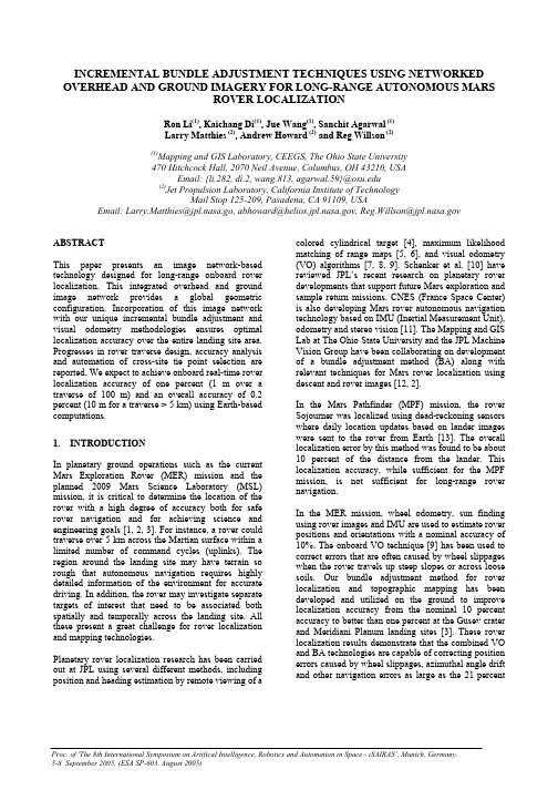
INCREMENTAL BUNDLE ADJUSTMENT TECHNIQUES USING NETWORKED OVERHEAD AND GROUND IMAGERY FOR LONG-RANGE AUTONOMOUS MARSROVER LOCALIZATIONRon Li(1), Kaichang Di(1), Jue Wang(1), Sanchit Agarwal (1)Larry Matthies (2), Andrew Howard (2) and Reg Willson (2)(1)Mapping and GIS Laboratory, CEEGS, The Ohio State University470 Hitchcock Hall, 2070 Neil Avenue, Columbus, OH 43210, USAEmail: {li.282, di.2, wang.813, agarwal.59}@(2)Jet Propulsion Laboratory, California Institute of TechnologyMail Stop 125-209, Pasadena, CA 91109, USAEmail: Larry.Matthies@jpl.nasa.go, abhoward@, Reg.Willson@ABSTRACTThis paper presents an image network-based technology designed for long-range onboard rover localization. This integrated overhead and ground image network provides a global geometric configuration. Incorporation of this image network with our unique incremental bundle adjustment and visual odometry methodologies ensures optimal localization accuracy over the entire landing site area. Progresses in rover traverse design, accuracy analysis and automation of cross-site tie point selection are reported. We expect to achieve onboard real-time rover localization accuracy of one percent (1 m over a traverse of 100 m) and an overall accuracy of 0.2 percent (10 m for a traverse > 5 km) using Earth-based computations.1. INTRODUCTIONIn planetary ground operations such as the current Mars Exploration Rover (MER) mission and the planned 2009 Mars Science Laboratory (MSL) mission, it is critical to determine the location of the rover with a high degree of accuracy both for safe rover navigation and for achieving science and engineering goals [1, 2, 3]. For instance, a rover could traverse over 5 km across the Martian surface within a limited number of command cycles (uplinks). The region around the landing site may have terrain so rough that autonomous navigation requires highly detailed information of the environment for accurate driving. In addition, the rover may investigate separate targets of interest that need to be associated both spatially and temporally across the landing site. All these present a great challenge for rover localization and mapping technologies.Planetary rover localization research has been carried out at JPL using several different methods, including position and heading estimation by remote viewing of a colored cylindrical target [4], maximum likelihood matching of range maps[5, 6], and visual odometry (VO) algorithms [7, 8, 9]. Schenker et al. [10] have reviewed JPL’s recent research on planetary rover developments that support future Mars exploration and sample return missions. CNES (France Space Center) is also developing Mars rover autonomous navigation technology based on IMU (Inertial Measurement Unit), odometry and stereo vision [11]. The Mapping and GIS Lab at The Ohio State University and the JPL Machine Vision Group have been collaborating on development of a bundle adjustment method (BA) along with relevant techniques for Mars rover localization using descent and rover images [12, 2].In the Mars Pathfinder (MPF) mission, the rover Sojourner was localized using dead-reckoning sensors where daily location updates based on lander images were sent to the rover from Earth [13]. The overall localization error by this method was found to be about 10 percent of the distance from the lander. This localization accuracy, while sufficient for the MPF mission, is not sufficient for long-range rover navigation.In the MER mission, wheel odometry, sun finding using rover images and IMU are used to estimate rover positions and orientations with a nominal accuracy of 10%. The onboard VO technique [9] has been used to correct errors that are often caused by wheel slippages when the rover travels up steep slopes or across loose soils. Our bundle adjustment method for rover localization and topographic mapping has been developed and utilized on the ground to improve localization accuracy from the nominal 10 percent accuracy to better than one percent at the Gusev crater and Meridiani Planum landing sites [3]. These rover localization results demonstrate that the combined VO and BA technologies are capable of correcting position errors caused by wheel slippages, azimuthal angle drift and other navigation errors as large as the 21 percentProc. of 'The 8th International Symposium on Artifical Intelligence, Robotics and Automation in Space - iSAIRAS’, Munich, Germany. 5-8 September 2005, (ESA SP-603, August 2005)error experienced within Eagle crater at the Meridiani Planum landing site and the 10.5 percent error experienced in the Husband Hill area at the Gusev crater landing site. Routinely produced orthoimages, DTMs (digital elevation models), and rover traverse maps have been provided to MER mission scientists and engineers through a web-based GIS that has greatly supported tactical and strategic mission operations [3, 14, 15].This paper describes an image network-based technology that has been designed for long-range onboard rover position localization (> 5 km). In Section 2, we introduce conceptualization and key components of the proposed rover localization technology and its operational considerations. Section 3 describes rover traverse design and theoretical analysis of localization accuracy. Section 4 reports on the initial results of rock modelling and matching for automated cross-site tie point selection. Section 5 gives conclusions and future research directions.Fig. 1. Networked overhead and ground imagery forlong-range rover localization.Benefits of using the bundle-adjusted image network include 1) high precision rover locations and rover paths even in an extended area over 5 km from the landing center; 2) accurate networked overhead and ground images with bundle-adjusted pointing parameters that are capable of supporting enhanced characterization of terrain features from multiple sensors and multiple views; and 3) global and local 3-D terrain models along with detailed accurate landmarks, rover paths, and mapping products in support of rover navigation and science instrument deployment anywhere on the site.2. IMAGE NETWORK-BASED TECHNOLOGYAND INCREMENTAL BUNDLE ADJUST-MENT TECHNIQUES FOR AUTONOMOUS MARS ROVER LOCALIZATIONThe image network will be established in a progressive way. High-resolution orbital images such as MOC NA in single or stereo forms will be prepared and processed before landing. During the landing process, overhead images will also be acquired and included in the network (if the mission is equipped with a descent imaging system). The ground (Navcam- and Pancam-like) images are acquired as the rover moves from site to site, containing complete or partial panoramas at each rover site connected by traversing images collected in between. Detailed close-range terrain features are used to tie the ground images and the low-level descent images (if available) while remote landmarks are utilized to link the ground images with the orbital images through use of the multi-resolution descent images. If descent images are not available, linkage of the orbital images with ground images will be achieved using the most distinguishable landmarks that can be identified and measured in both types of images.The proposed rover localization technology is based on incremental bundle adjustment of networked overhead and ground imagery. This image network will link overhead images (including orbital and descent images, if available) with ground images (including rover panoramic images and traversing images) through features on the ground and/or remote landmarks (Fig. 1). This integrated image network presents a much stronger geometry than other image-based localization methods. It thus ensures optimal rover localization accuracy over the entire landing site, both from onboard processing (real time, on Mars) and from ground-based processing (uplinked to the rover from Earth). This new technology includes the following three significant improvements over the technology used in the MER mission: (1) automation of the cross-site tie point selection process and development of an onboard version of the incremental BA software, (2) integration of the onboard incremental BA with VO to achieve long-range autonomous rover localization, and (3) development of an earth-based BA software system that integrates orbital and ground images of the entire image network to achieve optimal localization accuracy.3. ROVER TRAVERSE DESIGN ANDACCURACY ANALYSISThe design and error analysis of the rover traverse is of great importance. It will affect localization accuracy, automation of processes, and overall operational efficiency. Based on our previous rover traverse simulation study [16], we performed a systematic investigation of the potential for localization accuracy under different traverse configurations: distance between adjacent sites, number of tie points, convergence angles, etc. We used the following camera parameters in this analysis (Table 1). The analysis is first performed for the case of only two sites and then extended to a multiple-site scenario. We give only a brief summary of the results in this paper; technical details can be found in [17]. Fig. 2. Configuration of the onboard image network.The onboard rover positioning procedure will integrate VO and BA to achieve high efficiency and full automation. As illustrated in Fig. 2, BA is performed at waypoints (panoramic sites and mid-point survey positions), while VO is performed between waypoints. The BA obtains the following data from VO: tracked features, refined image-orientation parameters as an input, and first and last stereo pairs. After BA, rover positions are updated at subsequent waypoints.Table 1. Camera parameters used in accuracy analysis.MER Navcam MSL Pancam MER Navcam Stereo Base 20 cm 30 cm 30 cm Focal Length14.67 mm14.67 mm43 mmThe onboard localization system performs incremental rover localization in real time during each sol by processing only images acquired since the last uplink, i.e., images acquired on the same sol. During traversing, the onboard localization system can also provide bundle-adjusted image pointing data that may be used for autonomous hazard detection, 3-D local terrain mapping, and robotic decision making. The off-board bundle adjustment will process those images downlinked within the last few sols (e.g., three sols). This will be performed in an incremental manner. Rover position and attitude information is then updated through an uplink once the ground based BA is performed. Finally, the integrated bundle adjustment will adjust all available overhead images and downlinked ground images collected since Sol 1 to provide the optimal solution and the best accuracy of the network. This overall bundle adjustment is comprehensive and computationally intensive, and will be performed only every few sols to calibrate the uplinked rover positions and attitudes. We assume that landmarks (tie points) are evenly distributed in the middle of the two adjacent sites (Fig. 3 shows nine tie points as an example). Based on estimations of the range measurement error and azimuth measurement error and the error propagation principle, we estimated the rover localization error under different network configurations. Table 2 lists configurations of the image network that meet the desired one percent localization accuracy for different camera settings. The angle and length parameters in the table are the optimal convergence angle and traverse length, respectively.Because the overall geometry of the image network is controlled by the hierarchical image network that covers the entire region of rover operations, the accuracy of the bundle adjustment results for rover localization and mapping does not rapidly decrease or degrade as the rover traverses to remote areas of the landing site. The different levels of the bundle adjustment along with the strategy used for updating rover positions and attitudes ensure that the system will work in an environment of Mars landed missions such as MSL 2009. Fig. 3. Tie point distribution and convergence angle.Table 2. Image network configuration under assumption of rover localization accuracy (1 %) andtwo sitesImage networkconfigurationNo. of landmarks Convergenceangle andtraverselengthMERNavcamMSLNavcamMERPancam Angle (°) 71 71 712Length (m) 7.5 11.2 33Angle (°) 88 to 86 90 to 86 86 4Length (m) 19 28.6 85Angle (°) 86 to 84 88 to 84 84 to 83 6Length (m) 22 32.4 100Angle (°) 79 to 64 86 to 66 64 to 62 9Length (m) 26 38.8 118 Based on Table 2, we can draw the following conclusions for rover localization using two sites. (1) Rover localization error varies with the traverselength, number and distribution of tie points (landmarks), and camera system (stereo base, focal length, etc.).(2) In general, localization error is proportional to thesquare of the traverse length. In other words, relative localization error is proportional to the traverse length. Also, localization error decreases as either the base line or the focal length increase. (3) With 6 to 9 well-distributed tie points in the middleof two sites, rover localization error is within one percent at a traverse of 22 to 26 m for MER Navcam, a traverse of 32 to 39 m for MSL-type Navcam, or a traverse of 100 to 118 m with MER Pancam.To extend the two-site rover localization case to a multiple-site scenario, we apply the error propagation principle incrementally, site by site. Supposing the traverse lengths are the same for all adjacent sites, we evaluate the rover localization accuracy for a traverse of 5 km with different configurations. Results are summarized in Table 3.Table 3. Multiple-site rover traverse design anderror analysis for a 5 km traverse.CameraMERNavcamMSLNavcamMERPancamNo. of sites 194 130 44 Segment (leg) length 26 38.8 118No. of tie points atadjacent sites9 9 9 Relative localizationerror at two adjacentsites1 % 1 % 1 % Relative localizationerror of the 5 km traverse 0.072 % 0.088 % 0.15 %From Table 3, we can observe that if we keep anoptimal configuration for each traverse segment andcontrol the relative localization error within thesegment to one percent, an overall relative accuracy of0.1 to 0.2 percent can be achieved for a 5 km traverse.In the above analysis, target identification error (fromadjacent sites) was not taken into account. In general,the target identification error, the maximum of which isthe size of the target (e.g., a rock), is smaller than the3-D measurement error for far- and middle-rangetargets. If, when considering the target identificationerror, we suppose that localization error is double (i.e.,if localization error was two percent for one segment),an overall localization accuracy of 0.15 to 0.3 percentcould still be achievable for a 5 km traverse.4. AUTOMATION OF CROSS-SITE TIE POINTSELECTIONCurrently, we are developing a method for automaticcross-site tie point selection that consists of thefollowing four steps.(1) Landmark extraction: Automatic identification ofrocks from different sites in object space. We havecarried out experiments to detect rock peaks from3-D interest points and DTMs generated fromstereo pairs at an individual site.(2) Landmark modelling: Modelling the rock shapeconsidering invariance to position and lookingangle.(3) Landmark matching: Finding the correspondingrocks or rock patterns.(4) Tie point selection: Elimination of outliers andselection of well-distributed, reliable landmarks ascross-site tie points for bundle adjustment.The basic assumptions of our method are: 1)panoramas taken from two sites have sufficient overlapand the overlapping area is not too far from the cameracenter; 2) the area of overlap has some rocks (features)which stand out from the terrain; and 3) peaks, beingthe highest points of rocks, will always be visible fromdifferent angles.Rock peaks are extracted using the following criteria:1) they are the local maxima within a window of, e.g.,50 x 50 cm, 2) the maximum elevation differencewithin the window is greater than a threshold of 10 cm,and 3) there are at least three interest points within thewindow. We tested the algorithm using Navcampanoramic images acquired by the Spirit rover. Fig. 4shows the rock peaks (green dots) extracted from 3-Dinterest points of one stereo pair at two sites that are 5meters apart.Fig. 4. Rock peaks extracted from 3-D interest points.Fig. 6. Rock peaks extracted from twosites (5 meters apart).Fig. 5. Automatically matched rock peaks in stereopairs.The rock matching method is based on a Houghtransform-like initial matching and a heuristicrefinement. Currently, only rock peak information isused in the matching. When rock modelling task isfinished, the model information can be incorporated inthe matching process to improve the robustness andefficiency. Fig. 5 shows the matching result from therock peaks in Fig. 4. Eight peaks are matched for thestereo pair and all matches are corrected by visualchecking (Fig. 5).This same method has also been applied to two entire sites, MER-A 9946 and 10200. Extracted were 86 rock peaks in Site 9946 and 151 rock peaks in Site 10200 (Fig. 6). Twenty rock peaks were automatically matched and their distribution was fond to be good for bundle adjustment (Fig. 7). By visual checking, they were all found to be correct. This indicates that the rock extraction and matching methods worked well for sites close together. Experiments on sites far apart (26 m) have not been as successful as for those sites that are close together; only a few rock peaks could be matched in the area of overlap, and some mismatches occurred. The reason for mismatches is that some peak points are extracted at one site, but not at the other and they are mismatched with two other neighboring peak points at the second site. In order to obtain additional matched rocks, the rock extraction method must be enhanced.from two sites (5 meters apart).For rock modelling, we use rock shape and size information contained in extracted interest points to determine model parameters of the rocks. The idea is to establish analytical models of the rocks and to match corresponding model parameters from various sites to enhance rock peak matching.As described above, we are able to obtain the peaks of rocks from 3-D interest points. Starting from the peak of a particular rock, we try to identify more interest points in the vicinity of the peak that belong to that particular rock. Once we have sufficient 3-D points, we can model the shape of the rock. Fig. 8 shows an example of identified rock peaks and interest points on the rocks.Fig. 8. Rock peaks (green dots) and interest points (red dots) on the rocks.Currently we use a number of analytical models (e.g. hemisphere, semi-ellipsoid or cone) and determine the model whose parameters best fit the rock. Fig. 9 shows a semi-ellipsoid rock model that consists of three parameters: a, b, and h (Eq. 1). The parameters of a specific rock are calculated with a least-squares adjustment using the 3-D points on the rock.Fig. 9. Semi-ellipsoid rock model.1222=++hz b y a x (1)Fig. 10. Calculated parameters of rock models.We applied the rock modelling algorithm to the data shown in Fig. 8. Some examples of the calculated rock models are listed in Fig. 10. The model parametersobtained are compared with the actual dimensions of the rocks that are measured interactively. Height parameters match closely with actual rock heights. The accuracy of a and b parameters depends on the orientation of the rock in 3-D space. This should be considered when performing model matching. It should be noted that rock shapes could sometimes vary greatly. The chosen shape may not fit all rocks at a site. More experiments are needed to use several models for different rock types.5. CONCLUSIONSIn this paper, we have presented an image network-based technology designed for long-range onboard rover position localization. Through rover traverse design and accuracy analysis, we have found that with 6 to 9 well-distributed tie points distributed in the middle of two sites, rover localization error can be controlled within one percent at a traverse of 22 to 118 m, depending on camera settings. If we keep an optimal configuration for each traverse segment and control the relative localization error within that segment to one percent, an overall relative accuracy of 0.1 to 0.2 percent can be achieved for a 5 km traverse. The preliminary results of rock extraction and matching are satisfactory for sites close to each other (5 m). These methods of rock extraction, modelling and matching need to be enhanced to be effective for sites far apart (> 25 m). We expect to achieve full automation of cross-site tie point selection and enable a real-time incremental bundle adjustment for onboard rover localization, along with the proven ground based BA. zx6. ACKNOWLEDGEMENTSThis work has been supported by NASA/JPL through the Mars Technology Program. 7. REFERENCES1. Arvidson R.E., et al. Localization and physical properties experiments conducted by Spirit at Gusev Crater, Science , Special Issue on MER 2003 Mission, Vol. 305, No. 5685, 821-824, doi: 10.1126/science.1099922, 2004.2. Li R., Di K., Matthies, L.H., Arvidson R.E., Folkner W.M. and Archinal B.A., Rover localization and landing site mapping technology for 2003 Mars Exploration Rover mission, Photogrammetric Engineering & Remote Sensing , Vol. 70, No. 1, 77-90, 2004.3. Li R., et al. Initial Results of Rover Localization and Topographic Mapping for the 2003 Mars Exploration Rover Mission, PhotogrammetricEngineering & Remote Sensing, Special Issue on Mapping Mars, accepted, 2005.4. Volpe R., Litwin T. and Matthies L.H., MobileRobot Localization by Remote Viewing of a Colored Cylinder, Proceedings of the InternationalConference on Robots and Systems (IROS), Pittsburgh PA, August 5-9, 257-263, 1995.5. Olson C. and Matthies L., Maximum LikelihoodRover Localization by Matching Range Maps, Proceedings of the IEEE International Conferenceon Robotics and Automation, 272-277, 1998.6. Olson C., Probabilistic Self-Localization for MobileRobots, IEEE Transactions on Robotics and Automation, Vol. 16, No. 1, 55-66, 2000.7. Matthies L.H., Dynamic Stereo Vision, PhD thesis,Carnegie Mellon University, October, 1989.8. Olson C.F., Matthies L.H., Shoppers M. andMaimone M., Robust Stereo Ego-motion for LongDistance Navigation, In Proceedings of the IEEE Computer Society Conference on Computer Visionand Pattern Recognition, Vol.2, 453-458, 2000.9. Olson C.F., Matthies L.H., Shoppers M. andMaimone M., Rover navigation using stereo ego-motion, Robotics and Autonomous Systems, Vol.43, No.4, 215-229, 2003.10. Schenker P.S., Huntsberger T.L., Pirjanian P.,Baumgartner E.T., Tunstel E., Planetary Rover Developments Supporting Mars Exploration, Sample Return and Future Human-Robotic Colonization, Autonomous Robots, Vol. 14, No. 2-3, 103-126, 2003.11. Mauratte E., Mars Rover Autonomous Navigation,Autonomous Robots, Vol. 14, No. 2-3, 199-208, 2003.12. Li R., Ma F., Xu F., Matthies L.H., Olson C.F. andArvidson R.E., Localization of Mars Rovers UsingDescent and Surface-based Image Data, Journal ofGeophysical Research - Planets, Vol. 107, No. E11,FIDO 4.1 - 4.8, 2002.13. Matthies L., Gat E., Harrison R., Wilcox B., VolpeR. and Litwin T., Mars Microrover Navigation: Performance Evaluation and Enhancement, Autonomous Robots, Vol. 2, No.4, 291-311, 1995. 14. Li R., et al. Rover Localization and TopographicMapping at the Landing Site Of Gusev Crater, Mars, Journal of Geophysical Research - Planets,Special Issue on Spirit Rover, accepted, 2005.15. Li R., et al. Rover Localization and TopographicMapping at the Landing Site Of Meridiani Planum,Mars, Journal of Geophysical Research - Planets,Special Issue on Opportunity Rover, submitted, 2005.16. Di K., Li R., Matthies L. and Olson C., A Study onOptimal Design of Image Traverse Networks for Mars Rover Localization, Proceeding of ACSM-ASPRS 2002 Annual Conference, Washington,D.C., April 19-26, 2002. (CD-ROM). 17. Li R. and Di K., Rover traverse design and erroranalysis, report submitted to JPL Mars Technology Program, February 2005.。
Integrated density of states and Wegner estimates for random Schrodinger Operators
INTEGRATED DENSITY OF STATES AND WEGNER ESTIMATES
99
On the other hand, the electron could be moving in an amorphous medium, in which case there is no large group of symmetries of the Hamiltonian. However, from the physical point of view it is reasonable to assume that the local structure of the medium will be translation invariant on average. This means that we consider the potential which the electron experiences as a particular realisation of a random process and assume stationarity with respect to some group of translations. Moreover, physical intuition suggests to assume that the local properties of the medium in two regions far apart (on the microscopic scale) are approximately independent from each other. Therefore the stochastic process describing the potential should have a correlation function which decays to zero, or — more precisely — should be ergodic. There are interesting models which lie between the two extreme cases of latticeperiodic and amorphous media. They still have an underlying lattice structure which is, however, modified by disorder. Probably the best studied Hamiltonian with this properties is the alloy type model. We leave its precise definition for the next paragraph and introduce here a special case on the intuitive level. Consider first the potential Vω (x) := uk (ω, x) Each k corresponds to a nucleus sitting on a lattice point. The function uk (ω, ·) describes the atomic or nuclear potential at the site k and depends on the random parameter ω which models the different realisations of the configuration of the nuclei. If there is only one type of atom present, which has a spherically symmetric potential, all the uk (ω, ·) are the same, and Vω is periodic. Now assume that there are two kinds a and b of atoms present, which have spherically symmetric atomic potentials of the same shape, but which differ in their nuclear charge numbers. In this case the potential looks like Vω (x) :=
cfa三级笔记

cfa三级笔记Monte Carlo simulation(专题)定义:Monte Carlo simulation allows asset manager to model the uncertainty of several key variables. Generates random outcomes according to assumed probability distribution for these key variables. It is flexible approach for exploring different market or investment scenario. 蒙特卡洛模拟是将变量(事先定义好分布)的值随机发射,生成了结果,可灵活的探索不同市场、投资环境下的状态。
较MVO的优势:1, Rebalancing and taxes, Monte carlo simulation allow to analyze different rebalancing policies and their cost over time(in multi-period situation). 蒙特卡洛模拟可以用于分析执行不同的再平衡策略、税收时的影响。
2, Path dependent. As there are cash out flow each year, terminal wealth(the portfolio’s value at a given point)will be path-dependent because of the interaction of cash flows and returns. 如果每年都有资金流出,指定时间的组合价值会受这些资金流出和收益的影响Cash flows in and out of a portfolio and the sequence of returns will have a material effect on terminal wealth, this is termed path-dependent.3, Monte Carlo can incorporate statistical properties outside the normal distribution, such as skewness and excess kurtosis.蒙特卡洛模拟可用于建模非正态分布。
fluent操作界面中英
fluent 操作界面中英文对照Read 读取文件:scheme 方案journal 日志profile 外形 Write 保存文件Import :进入另一个运算程序 Interpolate :窜改,插入 Hardcopy : 复制, Batch options 一组选项 Save layout 保存设计Grid 网格Check 检查Info 报告:size 尺寸 ;memory usage 内存使用 情况;zones 区域;partitions 划分存储区 Polyhedral 多面体:Convert domain 变换范围Convert skewed cells 变换倾斜的单元Merge 合并 Separate 分割Fuse (Merge 的意思是将具有相同条件的边界合 并成一个;Fuse 将两个网格完全贴合的边界融合 成内部(interior)来处理,比如叶轮机中,计算多 个叶片时,只需生成一个叶片通道网格,其他通 过复制后,将重合的周期边界Fuse 掉就行了。
注意两个命令均为不可逆操作,在进行操作时注 意保存case) Zone 区域: append case file 添力口 case 文档 Replace 取代;delete 删除;deactivate 使复 位; Surface mesh 表面网孔Reordr 追加,添加:Domain 范围;zones 区域; Print bandwidth 打印 Scale 单位变换 Translate 转化Rotate 旋转 smooth/swap 光滑/交换CheckInfo ► Polyhedra►Merge...Separate ► Fuse...Zone►Surface Mesh... Reorder►Scale...Translate...Rotate...Smooth/Swap...ieGrid ] Define Solvea:w 1E3 SolverSolver* Pressure Based 'Density Based Space「2DL Axisymmetric 广 Axcsymmetric Swirl m 3DVelgty Formulatiqn • Absolute RelativeGradient Option区 Implicit「Explicit Time# SteadyUnsteadyPorous Formulation• Superficial VelocityPhysical Veiccity6K | Cancel] Help |Pressure based 基于压力 Density based 基于密度Models 模型:solver 解算器Formulation # Green-Gauss Cell Oased Green-Gauss N 。
锥拉伸与压缩不动点定理英文表示

锥拉伸与压缩不动点定理英文表示English:The Contraction Mapping Theorem, also known as the Banach Fixed-Point Theorem, states that for a complete metric space and a contraction mapping, there exists a unique fixed point. In other words, if there is a function that maps points in the space to other points such that the distance between the images of the points becomes smaller as the distance between the original points becomes smaller, then there exists a unique point in the space such that when the function is applied to this point, the result is the same point. This theorem is widely applicable in various fields such as economics, engineering, and computer science, where it is used to prove the existence and uniqueness of solutions to certain problems.中文翻译:收缩映射定理,也称为巴拿赫不动点定理,规定了在完备的度量空间和一个收缩映射下,存在一个唯一的不动点。
换句话说,如果存在一个函数,将空间中的点映射到其他点,使得原始点之间的距离变小时,它们的映射点之间的距离也变小,那么在空间中存在一个唯一的点,当该函数应用于该点时,结果仍然是同一个点。
无法收敛——精选推荐

⽆法收敛A dilation angle of 20.000 may result in decreasing plastic work or unstable material behavior at high confining stress states. Set the dilation angle less than 17.831 to ensure stable material behavior under all loading conditionsTHE SLAVE SURFACES ASSEMBLY__PICKEDSURF7 AND ASSEMBLY__PICKEDSURF9 INTERSECT EACH OTHER. THEY ARE PAIRED WITH MASTER SURFACES ASSEMBLY__PICKEDSURF6 ANDASSEMBLY__PICKEDSURF8 THAT ALSO INTERSECT EACH OTHER. IF BOTH PAIRS ARE *CONTACT PAIRs, THESE TWO PAIRS SHOULD NOT BE SIMULTANEOUSLY PRESENT IN A STEP BECAUSE OF POSSIBLE CONVERGENCE PROBLEMS; USE *MODEL CHANGE,TYPE=CONTACT PAIR TO REMOVE ONE OF THEM. IF BOTH ARE *TIE PAIRS, THE REDUNDANT TIES WILL BE REMOVED AUTOMATICALLY. IF ONE PAIR IS *TIE AND ANOTHER IS *CONTACT PAIR, REMOVE ONE OF THEM.THE SLAVE SURFACES ASSEMBLY__PICKEDSURF7 AND ASSEMBLY__PICKEDSURF11 INTERSECT EACH OTHER. THEY ARE PAIRED WITH MASTER SURFACES ASSEMBLY__PICKEDSURF6 ANDASSEMBLY__PICKEDSURF10 THAT ALSO INTERSECT EACH OTHER. IF BOTH PAIRS ARE *CONTACT PAIRs, THESE TWO PAIRS SHOULD NOT BE SIMULTANEOUSLY PRESENT IN A STEP BECAUSE OF POSSIBLE CONVERGENCE PROBLEMS; USE *MODEL CHANGE,TYPE=CONTACT PAIR TO REMOVE ONE OF THEM. IF BOTH ARE *TIE PAIRS, THE REDUNDANT TIES WILL BE REMOVED AUTOMATICALLY. IF ONE PAIR IS *TIE AND ANOTHER IS *CONTACT PAIR, REMOVE ONE OF THEM.THE SLAVE SURFACES ASSEMBLY__PICKEDSURF9 AND ASSEMBLY__PICKEDSURF11 INTERSECT EACH OTHER. THEY ARE PAIRED WITH MASTER SURFACES ASSEMBLY__PICKEDSURF8 ANDASSEMBLY__PICKEDSURF10 THAT ALSO INTERSECT EACH OTHER. IF BOTH PAIRS ARE *CONTACT PAIRs, THESE TWO PAIRS SHOULD NOT BE SIMULTANEOUSLY PRESENT IN A STEP BECAUSE OF POSSIBLE CONVERGENCE PROBLEMS; USE *MODEL CHANGE,TYPE=CONTACT PAIR TO REMOVE ONE OF THEM. IF BOTH ARE *TIE PAIRS, THE REDUNDANT TIES WILL BE REMOVED AUTOMATICALLY. IF ONE PAIR IS *TIE AND ANOTHER IS *CONTACT PAIR, REMOVE ONE OF THEM.For contact pair (assembly__pickedsurf7-assembly__pickedsurf6), adjustment was specified but no node was adjusted more than adjustment distance = 2.22000e-16.The ratio of the maximum incremental adjustment to the average characteristic length is 1.72284e-02 at node 1006 instance soil-1 on the surface pair (assembly__pickedsurf9,assembly__pickedsurf8).Not all the nodes that have been adjusted were printed. Specify *preprint,contact=yes for complete printout.For contact pair (assembly__pickedsurf11-assembly__pickedsurf10), adjustment was specified but no node was adjusted more than adjustment distance = 2.22000e-16.Please make sure that the mesh density of the slave surface in the tie pair(assembly__pickedsurf13,assembly__pickedsurf12) is finer than the master surface. The analysis may run slower, may yield inaccurate results, and may require more memory if this is not the case.For *tie pair (assembly__pickedsurf13-assembly__pickedsurf12), not all the nodes that have been adjusted were printed. Specify *preprint,model=yes for complete printout.72 nodes have been adjusted more than once. The subsequent adjustments may cause these nodes not to lie on their master surface. The nodes have been identified in node set WarnNodeAdjust.The nlgeom flag was not active in the previous general (non-perturbation) step. The activation of nlgeom in the current step may cause convergence problems if the displacements at the end of the previous general step are not small. Discontinuities in displacement response histories should also be expected.The plasticity/creep/connector friction algorithm did not converge at 936 pointsConvergence judged unlikely. Increment will be attempted again with a time increment of 0.25000The plasticity/creep/connector friction algorithm did not converge at 928 pointsConvergence judged unlikely. Increment will be attempted again with a time increment of 6.25000e-02 The plasticity/creep/connector friction algorithm did not converge at 666 pointsConvergence judged unlikely. Increment will be attempted again with a time increment of 1.56250e-02 The plasticity/creep/connector friction algorithm did not converge at 319 pointsConvergence judged unlikely. Increment will be attempted again with a time increment of 3.90625e-03 The plasticity/creep/connector friction algorithm did not converge at 36 pointsConvergence judged unlikely. Increment will be attempted again with a time increment of 3.29590e-03 The plasticity/creep/connector friction algorithm did not converge at 417 pointsConvergence judged unlikely. Increment will be attempted again with a time increment of 1.85394e-03 The plasticity/creep/connector friction algorithm did not converge at 44 pointsConvergence judged unlikely. Increment will be attempted again with a time increment of 4.63486e-04 The plasticity/creep/connector friction algorithm did not converge at 84 pointsConvergence judged unlikely. Increment will be attempted again with a time increment of 2.60711e-04 The plasticity/creep/connector friction algorithm did not converge at 52 pointsConvergence judged unlikely. Increment will be attempted again with a time increment of 9.77665e-05 The plasticity/creep/connector friction algorithm did not converge at 35 pointsConvergence judged unlikely. Increment will be attempted again with a time increment of 2.44416e-05 The plasticity/creep/connector friction algorithm did not converge at 20 pointsConvergence judged unlikely. Increment will be attempted again with a time increment of 1.00000e-05 The plasticity/creep/connector friction algorithm did not converge at 13 pointsConvergence judged unlikely. Increment will be attempted again with a time increment of 1.00000e-05 The plasticity/creep/connector friction algorithm did not converge at 12 points。
- 1、下载文档前请自行甄别文档内容的完整性,平台不提供额外的编辑、内容补充、找答案等附加服务。
- 2、"仅部分预览"的文档,不可在线预览部分如存在完整性等问题,可反馈申请退款(可完整预览的文档不适用该条件!)。
- 3、如文档侵犯您的权益,请联系客服反馈,我们会尽快为您处理(人工客服工作时间:9:00-18:30)。
Incremental Discretization for Naïve-Bayes ClassifierJingli Lu, Ying Yang and Geoffrey I. WebbClayton School of Information Technology, Monash UniversityVIC 3800, Australia{Jingli.Lu, Ying.Yang, Geoff.Webb}@.auAbstract.Naïve-Bayes classifiers (NB) support incremental learning. However, the lack ofeffective incremental discretization methods has been hindering NB’s incremental learning in faceof quantitative data. This problem is further compounded by the fact that quantitative data areeverywhere, from temperature readings to share prices. In this paper, we present a novelincremental discretization method for NB, incremental flexible frequency discretization(IFFD).IFFD discretizes values of a quantitative attribute into a sequence of intervals of flexible sizes. Itallows online insertion and splitting operation on intervals. Theoretical analysis and experimentaltest are conducted to compare IFFD with alternative methods. Empirical evidence suggests thatIFFD is efficient and effective. NB coupled with IFFD achieves a rapport between high learningefficiency and high classification accuracy in the context of incremental learning.1 IntroductionNaïve-Bayes classifiers (NB) are simple yet powerful [3, 4]. Its efficiency has witnessed its widespread deployment in real-world applications including medical diagnosis, fraud detection, email filtering and webpage prefetching. One key contributing factor to NB’s efficiency is its capability of incremental learning from qualitative data [5, 6]. To accommodate a new training instance, NB only needs to update relevant entries in its probability table. This often has a much lower cost than non-incremental approaches that have to rebuild a new classifier from scratch in order to include new training data.If learning involves quantitative data, NB often uses discretization to transform them into qualitative data. Briefly speaking, discretization groups sorted values of a quantitative attribute into intervals, treats each interval as a qualitative value and inputs them into NB. Ideally, discretization should also be incremental in order to be coupled with NB. When receiving a new training instance, incremental discretization is expected to be able to adjust intervals’ boundaries and statistics, using only the current intervals and this new instance instead of re-accessing previous training data. Unfortunately, the majority of existing discretization methods are not oriented to incremental learning. To update discretized intervals with new instances, they need to add those new instances into previous training data, and then re-discretize on basis of the updated complete training data set. This is detrimental to NB’s efficiency by inevitably slowing down its learning process. Hence there is a real and immediate need for appropriate incremental discretization methods for NB.Some preliminary research has been contributed to exploring incremental discretization for NB. A representative is the method PiD proposed by Gama and Pinto [6]. PiD is based on a two layer histograms and is efficient in term of time and space complexity. However it can be sub-optimal in that the histograms are not exact and the splitting operation in the first layer possibly produces inexact counters.This paper proposes a new effective approach, incremental flexible frequency discretization (IFFD). IFFD is based on fix frequency discretization (FFD) that has been demonstrated as a very efficient and effective discretization method for NB in the context of non-incremental learning [10, 11]. IFFD produces intervals with flexible sizes, stipulated by a lower bound and an upper bound. An interval is allowed to accept new values until its size reaches the upper bound. An interval whose size exceeds the upper bound is allowed to split if the resulting smaller intervals each have a size no smaller than the lower bound. Accordingly IFFD is able to incrementally adjust discretized intervals, effectively update associated statistics and efficiently synchronize with NB’s incremental learning.The remaining of this paper is organized as follows. Section 2 introduces naïve-Bayes learning and discretization. Section 3 explains the motivation and methodology of IFFD. Section 4 describes rival incremental methods from related work. Section 5 analyzes each alternative method’s complexity in terms of learning time and space. Section 6 conducts experiments to verify IFFD’s efficacy and efficiency. Section 7 gives concluding remarks.2 Discretization for Naïve-Bayes Learning2.1 Naïve-Bayes Classifier (NB)Assume that an instance I is a vector of attribute values <x 1, x 2, …, x n >, each value being an observation of an attribute X i (i ∈[1,n]). Each instance can have a class label c i },,,{21k c c c L ∈, being a value of the class variable C . If an instance has a known class label, it is a training instance. If an instance has no known class label, it is a testing instance. The dataset of training instances is called the training dataset. The dataset of testing instances is called the testing dataset.To classify an instance },,,{21n x x x I L =, NB estimates the probability of each class label given I , )|(I c C P i = using Formula (1, 2, 3,4). Formula (2) follows (1) because P (I ) is invariant across different class labels and can be canceled. Formula (4) follows (3) because of NB’s attributes independent assumption. It then assigns the class with the highest probability to I . NB is called naïve because it assumes that attributes are conditionally independent of each other given the class label. Although its assumption is sometimes violated, NB is able to offer surprisingly good classification accuracy in addition to its very high learning efficiency, which makes NB popular with numerous real-world classification applications [2, 8].)|(I c C P i = )()|()(I P c C I P c C P i i === )|()(i i c C I P c C P ==∝ )| xn , x2,x1,()(i i c C P c C P =><== ∏=====n j i j j i c C x XP c C P 1)|()((1)(2)(3)(4) In naïve-Bayes classifier, the class type must be qualitative while the attribute type can be either qualitative or quantitative. When an attribute X j is quantitative, it often has a large or even infinite number of values. As a result, the conditional probability that X j takes a particular value x j given the class label c i covers very few instance if there is any at all. Hence it is not reliable to estimate P (X j =x j |C=c i ) according to the observed instances. One common practice to solve the problem of quantitative data for NB is discretization.2.2 DiscretizationDiscretization is a popular approach to transforming quantitative attributes into qualitative ones for NB. It groups sorted values of a quantitative attribute into a sequence of intervals, treats each interval as a qualitative value, and maps every quantitative value into a qualitative value according to which interval it belongs to. In the paper, the boundaries among intervals are sometimes referred to as cut points . The number of instances in an interval is referred to as interval frequency . The total number of intervals produced by discretization is referred to as interval number .Incremental discretization aims at efficiently updating discretization intervals and associated statistics upon receiving each new training instance. Ideally, it does not require to access historical training instances to carry out the update. Instead it only needs the current intervals (with associated statistics) and the new instance.3 Incremental Flexible Frequency DiscretizationIn this section, we propose a novel incremental discretization method, incremental flexible frequency discretization (IFFD). It is motivated by the pros and cons of fixed frequency discretization (FFD) in the context of naive-Bayes learning and incremental learning [10, 11].3.1 Fixed Frequency Discretization (FFD)FFD has been proposed as an effective and efficient discretization method for naïve-Bayes learning through bias and variance management. It has been found that large interval size tends to increase NB’s classficiation bias while large interval number tends to increase NB’s classification variance [12]. To discretize a quantitative attribute, FFD sets a sufficient interval frequency, m = 30 [11,13]. It then discretizes the ascendingly sorted values into intervals of frequency m. By introducing m, FFD aims to ensure that each interval has sufficient training instances for NB probability estimation, reducing classification variance error. On top of that, by not limiting the number of intervals formed, more intervals can be formed as the training data size increases, reducing classification bias error. Empirical evidence has demonstrated that FFD helps NB achieve lower classification error than alternative discretization methods do.Although FFD is effective for naïve-Bayes learning, it is developed in the context of non-incremental learning. Every time when new training instances have arrived, FFD has to rebuild the discretization intervals from scratch. It is possible that even a single instance can push every boundary to (unnecessarily) move. For example, FFD discretizes the sorted values of a quantitative attribute into the following intervals. For simplicity, we assume m = 3:{3.0, 4.0, 4.3}, {4.5, 5.1, 5.9}, {6.0, 6.1, 6.2}, {6.5, 6.7, 6.8}, {6.9, 7.1} Suppose that a new instance has come with this attribute being value “5.2”. According to the current cut points, the appropriate interval to accommodate “5.2” is {4.5, 5.1, 5.9}. Inserting “5.2” into {4.5, 5.1, 5.9} will make the interval frequency increase to 4, which is greater than FFD’s specified threshold 3. Hence we need to move “5.9” out of the updated interval{4.5, 5.1, 5.2, 5.9} and insert it into the interval {6.0, 6.1, 6.2}, which produces another interval {5.9, 6.0, 6.1, 6.2} whose frequency is greater than 3. Following the same lines of reasoning, we have to move “6.2” into the next one and so on so forth until the last interval. As a result, the updated intervals are {3.0, 4.0, 4.3}, {4.5, 5.1, 5.2}, {5.9, 6.0, 6.1}, {6.2, 6.5, 6.7}, {6.8, 6.9, 7.1} and almost every cut point has been changed.In this case, FFD has to rebuild the intervals and NB’s conditional probability table from the second interval all the way to the last one. In the best situation, the new instance is inserted into the last interval and the computation cost can be non-trivial. However in the worst situation such as when the new instance is inserted into the first interval, FFD is extremely inefficient. The reason is that FFD specifies a fixed interval frequency. This observation motivates our new incremental discretization approach as follows.3.2 Incremental Flexible Frequency Discretization (IFFD)IFFD sets its interval frequency to be a range [minBinsize, maxBinsize) instead of a single value m. The two arguments, minBinsize and maxBinsize, are respectively the minimum and maximum frequency that IFFD allows intervals to assume. Whenever a new value arrives, IFFD first inserts it into the interval that the value falls into. IFFD then checks whether the updated interval’s frequency reaches maxBinsize. If not, it accepts the change and update statistics accordingly. If yes, IFFD splits the overflowed interval into two intervals under the condition that any of the resulting intervals has its frequency no less than minBinsize. Otherwise, even if the interval overflows because of the insertion, IFFD does not split it, in order to prevent high classification variance [10,11]. In the current implementation of IFFD, minBinsize is set as 30, following FFD’s lines of reasoning so as to minimize classification bias and variance; and maxBinsize is set as twice of minBinsize.By assuming a more flexible interval frequency, IFFD is able to solve FFD’s dilemma in incremental learning. Recall the example in Section 3.1. Assume minBinsize = 3 and hence maxBinsize = 6. When the new attribute value “5.2” comes, IFFD inserts it into the second interval {4.5, 5.1, 5.9}. That interval is hence changed into {4.5, 5.1, 5.2, 5.9} whose frequency (equal to 4) is still within [3, 6). So what we need do is only to modify NB’s conditional probabilies related to the second interval. Assume another two new attribute values “5.4, 5.5” have come and are again inserted into the second interval. This time, the interval {4.5, 5.1, 5.2, 5.4, 5.5, 5.9} has a frequency as 6, reaching maxBinSize. Hence IFFD will split it into {4.5, 5.1, 5.2} and {5.4, 5.5, 5.9} whose frequencies are both within [3, 6). Then we only need to recalculate NB’s conditional probabilities related to those two intervals. By this means, IFFD makes the update process local, affecting a minimum number of intervals and associated statistics. As a result, incremental discretization can be carried out very efficiently, Table 1 shows the pseudo codes of the IFFD algorithm. For simplicity, we just consider one attribute value to update the discretization intervals and classifier and assume all attribute values are different. cutPoints is the set of cut points of discretization intervals. counter is the conditional probability tableof the classifier. minBinsize is minimum bin size. IFFD will update the cutpoints and counter according to new attribute value V. classLabel is the class label of V.Table 1. Pseudo Codes of IFFDFunction: IFFD(cutPoints, counter, minBinsize, V, classLabel)//If V is greater than the last cut pointif(V > cutPoints[size-2] ) //size is the interval number// cutPoints counts from 0{ insert V into interval[size-1];counter[size-1][classLabel]++;chaInt = size-1; //record changed interval}else{ for(j = 0; j < size-1; j++)if(V =< cutPoints[j]){ insert V into interval[j];intFre[j]++;counter[j][classLabel]++; //update contingency tablechaInt = j; //record the interval which has been changedbreak;}}if(intFre[chaInt] > minBinsize*2){ get new cut point; //split interval[chaInt] into two c1 and c2 insert the new cut point into cutPoints;calculate counter[c1] and counter[c2];//update contingency table }Please be noted that identical values are always kept in the same interval. For example, if the interval is {4.5, 5.1, 5.2, 5.2, 5.2, 5.6, 5.9}, IFFD will not split it into {4.5, 5.1, 5.2} and {5.2, 5.6, 5.9} even though its frequency has exceeds maxBinsize (=6). Nor will IFFD split it into {4.5, 5.1} and {5.2, 5.2, 5.2, 5.6, 5.9} or {4.5, 5.1, 5.2, 5.2, 5.2} and {5.6, 5.9}, because the smaller interval frequency is less than minBinsize (=3).4 Rival Methods from Related Work4.1 Move Boundary FFD (MFFD)An intuitive way to relieve FFD’s dilemma in incremental learning (Section 3.1) is to just move the interval boundaries instead of redoing discretizaiton. We name this method move boundary FFD (MFFD). For the same example as in Section 3.1, if MFFD is applied, we just calculate the change of every interval. The second interval {4.5, 5.1, 5.9} has been inserted into an attribute value “5.2” and delete an attribute value “5.9”, then we just modify the conditional probability. Attention is only paid to the inserted and deleted values. Do like this until the last interval. NB coupled with MFFD has the same classification accuracy as NB coupled with FFD, but the former is more efficient than the latter.Table 2 presents the pseudo codes of MFFD. For simplicity, we just consider one attribute value to update the discretization intervals and classifier and assume all attribute values are different. cutpoints is the set of cut points of discretization intervals. counter is the conditional probability table of theclassifier. MFFD will update the c utpoints and counter according to new attribute value V. classLabel is the class label of V.Table 2. The Pseudo Codes of MFFDFunction: MFFD(cutPoints, counter, V, classLabel)curVal=V; curClasslabel= classLabel;for(j = 0; j < size-1; j++) //size is the interval number{ if(curVal =< cutpoints[j]){ // interval[j] is the jth interval of the attributeinsert curVal into interval[j];//fre is the specified interval frequency// V[j][fre-1]is the last value in interval[j]remove V[j][fre-1]from interval[j];cutPoints[j]= V[j][fre-2]; //modify cut pointscounter[j][curClasslabel]++; //update contingency table]--;counter[j][ V[j][fre-1].classcurVal = V[j][fre-1];curClasslabel = V[j][fre-1];.class}}If(fre[size-1] < split threshold){ insert curVal into interval[size-1];counter[size-1][curClasslabel]++;}else{ split interval[size-1];calculate counter[size-1] and counter[size];size = size+1;}4.2 Partition Incremental Discretization (PiD)PiD is a two layer histograms incremental discretization method [6]. The first layer based on equal-width or equal-frequency determines the candidate cut points according to observed values. At this layer, the interval number is significantly greater that the final interval number. For example, the final interval number is 40, probably the interval number in the first layer is 200. For incremental learning, it inserts the incremental data into the appropriate intervals. To any interval whose frequency is greater than the specified threshold, it will be split. Because in this layer, it does not store the historical data, the splitting result is inaccurate. It just splits an interval into two uniformly. The second layer merges the intervals gained at the first layer. In the second layer, PiD can construct the final discretization interval by any different strategies. Namely, PiD discretizes quantitative attributes twice. At first, it uses a loose interval number to discretize; and then merges intervals if necessary. The main advantage of PiD is low time and space complexity, but during the splitting operation in the first layer, it possibly produces inexact counters.4.3 Kernel Density Estimation (KDE)A counterpart of discretization is probability density estimation to handle quantitative attributes for NB. It models each quantitative attribute by some continuous probability distribution. Probabilitydensity estimation methods can manipulate quantitative attributes for naïve-Bayes incremental learning. A representative method is kernel density estimation (KDE) [7].KDE is a non-parametric approach that does not assume the underlying distribution to take any particular form. Instead it estimates from sample values. This circumvents unsafe assumptions and achieves better accuracy because of real world diversity. For KDE, it calculates the conditional class probability as:∑∫===k h l j c k j i i j j dx x f n c C x X P ),,(1)|(σµ (5)where n i is the number of training instances with class label c i . For every quantitative attribute of testing instance, KDE has to perform probability calculation n i times to get P (X j =x j |C=c i ). If the instance number is large, it has a potential computational problem.5 Time and Space Complexity ComparisonIn this section, we analyse the time and space complexity incurred by accommodating a new training instance. It includes updating the discretized intervals as well as updating required probabilities for NB.5.1 Time ComplexityIn the following, n is abbreviation of instance number; k is the attribute number; C is the number of class label, specified Interval Frequency is abbreviated by IntF , IntN represents Interval Number , then IntN =n/IntF .5.1.1 Train Time Complexity on a New InstanceTrain Time Complexity of MFFDAssume the probability of the new attribute value inserting into every interval is equal. 1+−i IntN is the number of intervals which has to be changed, where i is the appropriate interval for the new instance. Inserting an instance into the interval while deleting another one from the interval has a constant cost in time complexity O(1). So for every incremental attribute value, the training time complexity is presents in equation (6). This complexity repeating for k attribute is O(k), so resulting in the totally complexity is O(n)*O(k)=O(nk).).(O(1)*21O(1)*21O(1)*2)1(O(1)*)1(1n O IntF n IntN IntN IntN IntN IntN i IntN IntN i =+=+=+=+−∑= (6)Train Time Complexity of PiDThe time complexity of PiD depends on the discretization methods selected in each layer. In our experiments, we select equal-width and PD for the two layers separately (the reason that we select them is explained in 4.2.1). Here we just analyze time complexity in this situation.In the first layer, when the interval frequency of a specified interval is greater than a user defined threshold ( a percentage of the total instance number), the interval will be split. The more interval number is defined in the first layer, the less probability some interval will be split. In the first layer, the interval frequency is a large number, so the time for splitting operation can be ignored. The input of the second layer is the intervals and associated statistics of first layer. If the interval gained in the first layer is m , then the time complexity of PiD is O (mk ).Train Time Complexity of IFFDAssume the probability of the new attribute value inserting into some interval is equal. Max is the maximum interval frequency; Min is the minimum interval frequency.When a new attribute value inserts into the appropriate interval, the probability that the interval does not split is 1+−−Min Max Min Max . In this situation, the operation is just to insert the new instance. Inserting an instance into the interval has a constant cost in time complexity O(1). The probability that the interval splits is 11+−Min Max . In this situation, the operation is to recalculate the conditional probability table of the two new intervals and change the cut points. For a single attribute, if the data structure ofcutPoints is array, the time complexity is presented in equation (7), 2IntN means the number of cut points have to move, when insert a new cut point into the cutPoints . And if tree or list structure is selected, the time complexity is demonstrated as equation (8). This complexity repeating for k attribute is O(k), so resulting in the totally complexity for array structure is O(n)*O(k)=O(nk) and for tree structure is O(1)*O(k)=O(k). In our experiment, we select array structure to store cutPoints , because our select Weka as the platform, in Weka, cutPoints is stored in an array.).()21(*111O(1)*)(n O IntN Min Min Max Min Max Min Max =+++−++−− ).1(2112111O(1)*)(O Min Min Min Max Min Min Max Min Max =≈++=+−+++−− (7)(8) Train Time Complexity of KDEAt training time, KDE just store the attribute values, so its time complexity is O (k ).5.1.2 Test Time Complexity on a New InstanceTest Time Complexity of MFFD, IFFD and PiDFor every class label, the classifiers which manipulate quantitative attributes by discretization methods can get the conditional probability from the conditional probability table directly, so testing time complexity on the new instance is O (Ck ).Test Time Complexity of KDEAt testing time, from equation (5) we can see, for every class label c i and every quantitative attributes, KDE must evaluate f for every observed different attribute value whose class label is in class c i . So the testing time complexity of KDE is O (nk ).5.2 Space Complexity5.2.1 Space Complexity of MFFD, IFFD & KDE on a New InstanceMFFD, IFFD and KDE have to store the historical quantitative attributes, so their space complexity is O (nk ).MFFD has to change the cut points and modify the conditional probability table, so historical quantitative attributes are necessary.For IFFD, when the interval frequency of some interval exceeds the threshold, the interval has to be split. Historical quantitative data is necessary to splitting operation. So IFFD must store the historical quantitative attribute values for every instance. But for every new instance, the modified interval is just one: split it or insert a point into it, namely the adjustment is local. So we can store the historical data in external storage. When change is necessary, we copy it from external storage to memory. With the development of hardware, storage is not a big problem.KDE must store every different quantitative attribute value for every class label. To classify an instance, KDE has to access every attribute value to calculate the conditional class probability. So it is necessary to store the attributes values in the memory. However memory store is more expensive than external storage. If for every class label there are many duplicate quantitative attribute values, KDE has a lower space then MFFD and IFFD; otherwise their storage space are equal.5.2.2 Space Complexity of PiD on a New InstanceSplitting operation in PiD is to split an interval uniformly. PiD does not need to store historical quantitative attribute values. It just stores the interval information which gained at the first layer. So its space complexity is O(m), where m is the number of interval in the first layer. Compared with other methods, PiD has the lowest space complexity.The time and space complexity are summarized in Table 3.Table 3. Algorithmic complexity. n is abbreviation of instance number; k is the attribute number; C is the number of class label; m is the number of interval number in the first layer for PiDMethod MFFD IFFD PiD KDETrainning O(nk) O(nk) (Array)O(k) (Tree) O(mk) O(k)TimeComplexityTesting O(Ck) O(Ck) O(Ck) O(nk)Space Complexity O(nk) O(nk) O(mk) O(nk)6 Experimental EvaluationIn this section, we compare the incremental learning performance of NB when coupled with IFFD, PiD, MFFD and KDE respectively to handle quantitative attributes.6.1 DataThe experiments use a large suite of 30 benchmark datasets from the UCI machine learning repository [1]. For the purpose of incremental learning, the chosen datasets each have more than 500 instances. Table 4 describes the statistics of each dataset.Table 4. Experimental Datasets. For each dataset, Size is the number of instances, Qa is the number of quantitative attributes, Ql is the number of qualitative attributes and C is the number of classes.ID Dataset Size Qa Ql C ID Dataset Size Qa Ql C1 cylinder-bands 540 20 192 16 Abalone 4177 8 0 32 balance-scale 625 4 03 17 spambase 4601 57 0 23 credit-a 690 6 9 2 18 waveform-5000 5000 40 0 34 breast-w 699 9 0 2 19 page-blocks 5473 10 0 55 diabetes 768 8 0 2 20 optdigits 5620 48 0 106 vehicle 846 18 0 4 21 satellite 6435 36 0 67 anneal 898 6 32 6 22 Musk2 6598 166 0 28 vowel 990 10 3 11 23 pioneer 9150 30 6 579 German 1000 7 13 2 24 Thyroid 9169 7 22 2010 cmc 1473 2 7 3 25 ae 9961 12 0 911 yeast 1484 7 1 10 26 pendigits 1099216 0 1012 volcanoes 1520 3 0 4 27 Sign 125468 0 313 mfeat-zernike 2000 47 0 10 28 letter 2000016 0 2614 segment 2310 19 0 7 29 Adult 48842 6 8 215 hypothyroid 3772 7 23 4 30 Shuttle 580009 0 76.2 DesignFor each instance, we randomly shuffle the instances and use the first 200 instances to initialize an NB classifier. The remaining instances come one after the other. Each instance is to be classified by the current NB first. Its true class label is then made known to the classifier which takes it as a new training instance. Accordingly, the discretized intervals are updated and so is the classifier. Then the next instance comes and the same procedure runs again, and so on so forth until the last instance is classified. We call this complete process a trial. We conduct five trails and average their classification error rates.。