Theory of magnetic short-range order for itinerant electron systems
磁共振(磁谐振耦合)无线充电技术鼻祖级文章-英文原文

Wireless Power Transfer via Strongly Coupled Magnetic ResonancesAndré Kurs,1* Aristeidis Karalis,2 Robert Moffatt,1 J. D. Joannopoulos,1 Peter Fisher,3Marin Soljačić11Department of Physics, Massachusetts Institute of Technology, Cambridge, MA 02139, USA. 2Department of Electrical Engineering and Computer Science, Massachusetts Institute of Technology, Cambridge, MA 02139, USA. 3Department of Physics and Laboratory for Nuclear Science, Massachusetts Institute of Technology, Cambridge, MA 02139, USA.*To whom correspondence should be addressed. E-mail: akurs@Using self-resonant coils in a strongly coupled regime, we experimentally demonstrate efficient non-radiative power transfer over distances of up to eight times the radius of the coils. We demonstrate the ability to transfer 60W with approximately 40% efficiency over distances in excess of two meters. We present a quantitative model describing the power transfer which matches the experimental results to within 5%. We discuss practical applicability and suggest directions for further studies. At first glance, such power transfer is reminiscent of the usual magnetic induction (10); however, note that the usual non- resonant induction is very inefficient for mid-range applications.Overview of the formalism. Efficient mid-range power transfer occurs in particular regions of the parameter space describing resonant objects strongly coupled to one another. Using coupled-mode theory to describe this physical system (11), we obtain the following set of linear equationsIn the early 20th century, before the electrical-wire grid, Nikola Tesla (1) devoted much effort towards schemes to a&m(t)=(iωm-Γm)a m(t)+∑iκmn a n(t)+F m(t)n≠m(1)transport power wirelessly. However, typical embodiments (e.g. Tesla coils) involved undesirably large electric fields. During the past decade, society has witnessed a dramatic surge of use of autonomous electronic devices (laptops, cell- phones, robots, PDAs, etc.) As a consequence, interest in wireless power has re-emerged (2–4). Radiative transfer (5), while perfectly suitable for transferring information, poses a number of difficulties for power transfer applications: the efficiency of power transfer is very low if the radiation is omnidirectional, and requires an uninterrupted line of sight and sophisticated tracking mechanisms if radiation is unidirectional. A recent theoretical paper (6) presented a detailed analysis of the feasibility of using resonant objects coupled through the tails of their non-radiative fields for mid- range energy transfer (7). Intuitively, two resonant objects of the same resonant frequency tend to exchange energy efficiently, while interacting weakly with extraneous off- resonant objects. In systems of coupled resonances (e.g. acoustic, electro-magnetic, magnetic, nuclear, etc.), there is often a general “strongly coupled” regime of operation (8). If one can operate in that regime in a given system, the energy transfer is expected to be very efficient. Mid-range power transfer implemented this way can be nearly omnidirectional and efficient, irrespective of the geometry of the surrounding space, and with low interference and losses into environmental objects (6).Considerations above apply irrespective of the physical nature of the resonances. In the current work, we focus on one particular physical embodiment: magnetic resonances (9). Magnetic resonances are particularly suitable for everyday applications because most of the common materials do not interact with magnetic fields, so interactions with environmental objects are suppressed even further. We were able to identify the strongly coupled regime in the system of two coupled magnetic resonances, by exploring non-radiative (near-field) magnetic resonant induction at MHzfrequencies. where the indices denote the different resonant objects. The variables a m(t) are defined so that the energy contained in object m is |a m(t)|2, ωm is the resonant frequency of thatisolated object, and Γm is its intrinsic decay rate (e.g. due to absorption and radiated losses), so that in this framework anuncoupled and undriven oscillator with parameters ω0 and Γ0 would evolve in time as exp(iω0t –Γ0t). The κmn= κnm are coupling coefficients between the resonant objects indicated by the subscripts, and F m(t) are driving terms.We limit the treatment to the case of two objects, denoted by source and device, such that the source (identified by the subscript S) is driven externally at a constant frequency, and the two objects have a coupling coefficient κ. Work is extracted from the device (subscript D) by means of a load (subscript W) which acts as a circuit resistance connected to the device, and has the effect of contributing an additional term ΓW to the unloaded device object's decay rate ΓD. The overall decay rate at the device is therefore Γ'D= ΓD+ ΓW. The work extracted is determined by the power dissipated in the load, i.e. 2ΓW|a D(t)|2. Maximizing the efficiency η of the transfer with respect to the loading ΓW, given Eq. 1, is equivalent to solving an impedance matching problem. One finds that the scheme works best when the source and the device are resonant, in which case the efficiency isThe efficiency is maximized when ΓW/ΓD= (1 + κ2/ΓSΓD)1/2. It is easy to show that the key to efficient energy transfer is to have κ2/ΓSΓD> 1. This is commonly referred to as the strongcoupling regime. Resonance plays an essential role in thisDS S D'' power transfer mechanism, as the efficiency is improved by approximately ω2/ΓD 2 (~106 for typical parameters) compared to the case of inductively coupled non-resonant objects. Theoretical model for self-resonant coils. Ourexperimental realization of the scheme consists of two self- resonant coils, one of which (the source coil) is coupled inductively to an oscillating circuit, while the other (the device coil) is coupled inductively to a resistive load (12) (Fig. 1). Self-resonant coils rely on the interplay between distributed inductance and distributed capacitance to achieve resonance. The coils are made of an electrically conducting wire of total length l and cross-sectional radius a wound into Given this relation and the equation of continuity, one finds that the resonant frequency is f 0 = 1/2π[(LC )1/2]. We can now treat this coil as a standard oscillator in coupled-mode theory by defining a (t ) = [(L /2)1/2]I 0(t ).We can estimate the power dissipated by noting that the sinusoidal profile of the current distribution implies that the spatial average of the peak current-squared is |I 0|2/2. For a coil with n turns and made of a material with conductivity σ, we modify the standard formulas for ohmic (R o ) and radiation (R r ) µ0ω l a helix of n turns, radius r , and height h . To the best of our knowledge, there is no exact solution for a finite helix in the literature, and even in the case of infinitely long coils, the solutions rely on assumptions that are inadequate for our R o = 2σ 4πa µ πωr 42 ωh 2 (6)system (13). We have found, however, that the simple quasi- R =0 n 2 + (7)static model described below is in good agreementr ε 12 c3π3 c(approximately 5%) with experiment.We start by observing that the current has to be zero at the ends of the coil, and make the educated guess that the resonant modes of the coil are well approximated bysinusoidal current profiles along the length of the conducting wire. We are interested in the lowest mode, so if we denote by s the parameterization coordinate along the length of the conductor, such that it runs from -l /2 to +l /2, then the time- dependent current profile has the form I 0 cos(πs /l ) exp(i ωt ). It follows from the continuity equation for charge that the linear charge density profile is of the form λ0 sin(πs /l ) exp(i ωt ), so the two halves of the coil (when sliced perpendicularly to its axis) contain charges equal in magnitude q 0 = λ0l /π but opposite in sign.As the coil is resonant, the current and charge density profiles are π/2 out of phase from each other, meaning that the real part of one is maximum when the real part of the other is zero. Equivalently, the energy contained in the coil is 0The first term in Eq. 7 is a magnetic dipole radiation term(assuming r << 2πc /ω); the second term is due to the electric dipole of the coil, and is smaller than the first term for our experimental parameters. The coupled-mode theory decay constant for the coil is therefore Γ = (R o + R r )/2L , and its quality factor is Q = ω/2Γ.We find the coupling coefficient κDS by looking at the power transferred from the source to the device coil,assuming a steady-state solution in which currents and charge densities vary in time as exp(i ωt ).P =⎰d rE (r )⋅J (r ) =-⎰d r (A&S (r )+∇φS (r ))⋅J D (r ) at certain points in time completely due to the current, and at other points, completely due to the charge. Usingelectromagnetic theory, we can define an effective inductance L and an effective capacitance C for each coil as follows:=-1⎰⎰d r d r ' µJ &S(r ')+ρS(r ') 4π |r -r |ε0≡-i ωMI S I Dr '-r|r '-r |3⋅J D (r )(8)L =µ04π |I 0 |⎰⎰d r d r 'J (r )⋅J (r ')|r -r '|where the subscript S indicates that the electric field is due to the source. We then conclude from standard coupled-mode theory arguments that κDS = κSD = κ = ωM /2[(L S L D )1/2]. When 1 1 ρ(r )ρ(r ') the distance D between the centers of the coils is much larger= C 4πε 0 |q 0 | ⎰⎰d r d r ' |r -r '|(4)than their characteristic size, κ scales with the D -3dependence characteristic of dipole-dipole coupling. Both κ and Γ are functions of the frequency, and κ/Γ and the where the spatial current J (r ) and charge density ρ(r ) are obtained respectively from the current and charge densities along the isolated coil, in conjunction with the geometry of the object. As defined, L and C have the property that the efficiency are maximized for a particular value of f , which is in the range 1-50MHz for typical parameters of interest. Thus, picking an appropriate frequency for a given coil size, as we do in this experimental demonstration, plays a major role in optimizing the power transfer.1 2Comparison with experimentallydeterminedU =2 L |I 0 |parameters. The parameters for the two identical helical coils built for the experimental validation of the power 1 2 transfer scheme are h = 20cm, a = 3mm, r = 30 cm, and n = =2C|q 0 | (5)5.25. Both coils are made of copper. The spacing between loops of the helix is not uniform, and we encapsulate theuncertainty about their uniformity by attributing a 10% (2cm) uncertainty to h . The expected resonant frequency given these22dimensions is f0 = 10.56 ± 0.3MHz, which is about 5% off from the measured resonance at 9.90MHz.The theoretical Q for the loops is estimated to be approximately 2500 (assuming σ = 5.9 × 10⁷ m/Ω) but the measured value is Q = 950±50. We believe the discrepancy is mostly due to the effect of the layer of poorly conductingcopper oxide on the surface of the copper wire, to which the current is confined by the short skin depth (~20μm) at this frequency. We therefore use the experimentally observed Q and ΓS= ΓD= Γ = ω/2Q derived from it in all subsequent computations.We find the coupling coefficient κ experimentally by placing the two self-resonant coils (fine-tuned, by slightly adjusting h, to the same resonant frequency when isolated) a distance D apart and measuring the splitting in the frequencies of the two resonant modes. According to coupled-mode theory, this splitting should be ∆ω = 2[(κ2-Γ2)1/2]. In the present work, we focus on the case where the two coils are aligned coaxially (Fig. 2), although similar results are obtained for other orientations (figs. S1 and S2).Measurement of the efficiency. The maximum theoretical efficiency depends only on the parameter κ/[(L S L D)1/2] = κ/Γ, which is greater than 1 even for D = 2.4m (eight times the radius of the coils) (Fig. 3), thus we operate in the strongly- coupled regime throughout the entire range of distances probed.As our driving circuit, we use a standard Colpitts oscillator whose inductive element consists of a single loop of copper wire 25cm in radius(Fig. 1); this loop of wire couples inductively to the source coil and drives the entire wireless power transfer apparatus. The load consists of a calibrated light-bulb (14), and is attached to its own loop of insulated wire, which is placed in proximity of the device coil and inductively coupled to it. By varying the distance between the light-bulb and the device coil, we are able to adjust the parameter ΓW/Γ so that it matches its optimal value, given theoretically by (1 + κ2/Γ2)1/2. (The loop connected to the light-bulb adds a small reactive component to ΓW which is compensated for by slightly retuning the coil.) We measure the work extracted by adjusting the power going into the Colpitts oscillator until the light-bulb at the load glows at its full nominal brightness.We determine the efficiency of the transfer taking place between the source coil and the load by measuring the current at the mid-point of each of the self-resonant coils with a current-probe (which does not lower the Q of the coils noticeably.) This gives a measurement of the current parameters I S and I D used in our theoretical model. We then compute the power dissipated in each coil from P S,D=ΓL|I S,D|2, and obtain the efficiency from η = P W/(P S+ P D+P W). To ensure that the experimental setup is well described by a two-object coupled-mode theory model, we position the device coil such that its direct coupling to the copper loop attached to the Colpitts oscillator is zero. The experimental results are shown in Fig. 4, along with the theoretical prediction for maximum efficiency, given by Eq. 2. We are able to transfer significant amounts of power using this setup, fully lighting up a 60W light-bulb from distances more than 2m away (figs. S3 and S4).As a cross-check, we also measure the total power going from the wall power outlet into the driving circuit. The efficiency of the wireless transfer itself is hard to estimate in this way, however, as the efficiency of the Colpitts oscillator itself is not precisely known, although it is expected to be far from 100% (15). Still, the ratio of power extracted to power entering the driving circuit gives a lower bound on the efficiency. When transferring 60W to the load over a distance of 2m, for example, the power flowing into the driving circuit is 400W. This yields an overall wall-to-load efficiency of 15%, which is reasonable given the expected efficiency of roughly 40% for the wireless power transfer at that distance and the low efficiency of the Colpitts oscillator.Concluding remarks. It is essential that the coils be on resonance for the power transfer to be practical (6). We find experimentally that the power transmitted to the load drops sharply as either one of the coils is detuned from resonance. For a fractional detuning ∆f/f0 of a few times the inverse loaded Q, the induced current in the device coil is indistinguishable from noise.A detailed and quantitative analysis of the effect of external objects on our scheme is beyond the scope of the current work, but we would like to note here that the power transfer is not visibly affected as humans and various everyday objects, such as metals, wood, and electronic devices large and small, are placed between the two coils, even in cases where they completely obstruct the line of sight between source and device (figs. S3 to S5). External objects have a noticeable effect only when they are within a few centimeters from either one of the coils. While some materials (such as aluminum foil, styrofoam and humans) mostly just shift the resonant frequency, which can in principle be easily corrected with a feedback circuit, others (cardboard, wood, and PVC) lower Q when placed closer than a few centimeters from the coil, thereby lowering the efficiency of the transfer.When transferring 60W across 2m, we calculate that at the point halfway between the coils the RMS magnitude of the electric field is E rms= 210V/m, that of the magnetic field isH rms= 1A/m, and that of the Poynting vector is S rms=3.2mW/cm2 (16). These values increase closer to the coils, where the fields at source and device are comparable. For example, at distances 20cm away from the surface of the device coil, we calculate the maximum values for the fields to be E rms= 1.4kV/m, H rms= 8A/m, and S rms= 0.2W/cm2. The power radiated for these parameters is approximately 5W, which is roughly an order of magnitude higher than cell phones. In the particular geometry studied in this article, the overwhelming contribution (by one to two orders of magnitude) to the electric near-field, and hence to the near- field Poynting vector, comes from the electric dipole moment of the coils. If instead one uses capacitively-loaded single- turn loop design (6) - which has the advantage of confining nearly all of the electric field inside the capacitor - and tailors the system to operate at lower frequencies, our calculations show (17) that it should be possible to reduce the values cited above for the electric field, the Poynting vector, and the power radiated to below general safety regulations (e.g. the IEEE safety standards for general public exposure(18).) Although the two coils are currently of identical dimensions, it is possible to make the device coil small enough to fit into portable devices without decreasing the efficiency. One could, for instance, maintain the product of the characteristic sizes of the source and device coils constant, as argued in (6).We believe that the efficiency of the scheme and the power transfer distances could be appreciably improved by silver-plating the coils, which should increase their Q, or by working with more elaborate geometries for the resonant objects (19). Nevertheless, the performance characteristics of the system presented here are already at levels where they could be useful in practical applications.References and Notes1. N. Tesla, U.S. patent 1,119,732 (1914).2.J. M. Fernandez, J. A. Borras, U.S. patent 6,184,651(2001).3.A. Esser, H.-C. Skudelny, IEEE Trans. Indust. Appl. 27,872(1991).4.J. Hirai, T.-W. Kim, A. Kawamura, IEEE Trans. PowerElectron. 15, 21(2000).5.T. A. Vanderelli, J. G. Shearer, J. R. Shearer, U.S. patent7,027,311(2006).6.A. Karalis, J. D. Joannopoul os, M. Soljačić, Ann. Phys.,10.1016/j.aop.2007.04.017(2007).7.Here, by mid-range, we mean that the sizes of the deviceswhich participate in the power transfer are at least a few times smaller than the distance between the devices. For example, if the device being powered is a laptop (size ~ 50cm), while the power source (size ~ 50cm) is in thesame room as the laptop, the distance of power transfer could be within a room or a factory pavilion (size of the order of a fewmeters).8. T. Aoki, et al., Nature 443, 671 (2006).9.K. O’Brien, G. Scheible, H. Gueldner, 29th AnnualConference of the IEEE 1, 367(2003).10.L. Ka-Lai, J. W. Hay, P. G. W., U.S. patent7,042,196(2006).11.H. Haus, Waves and Fields in Optoelectronics(Prentice- Supporting Online Material/cgi/content/full/1143254/DC1SOM TextFigs. S1 to S530 March 2007; accepted 21 May 2007Published online 7 June 2007; 10.1126/science.1143254 Include this information when citing this paper.Fig. 1. Schematic of the experimental setup. A is a single copper loop of radius 25cm that is part of the driving circuit, which outputs a sine wave with frequency 9.9MHz. S and D are respectively the source and device coils referred to in the text. B is a loop of wire attached to the load (“light-bulb”). The various κ’s represent direct couplings between the objects indicated by the arrows. The angle between coil D and the loop A is adjusted to ensure that their direct coupling is zero, while coils S and D are aligned coaxially. The direct couplings between B and A and between B and S are negligible.Fig. 2. Comparison of experimental and theoretical values for κ as a function of the separation between coaxially aligned source and device coils (the wireless power transfer distance.) Fig. 3. Comparison of experimental and theoretical values for the parameter κ/Γ as a function of the wireless power transfer distance. The theory values are obtained by using the theoretical κ and the experimentally measured Γ. The shaded area represents the spread in the theoretical κ/Γ due to the 5% uncertainty in Q.Fig. 4. Comparison of experimental and theoretical efficiencies as functions of the wireless power transfer distance. The shaded area represents the theoretical prediction for maximum efficiency, and is obtained by inserting theHall, Englewood Cliffs, NJ, 1984).12.The couplings to the driving circuit and the load donot theoretical values from Fig. 3 into Eq. 2 [with Γκ2/Γ2 1/2 W /ΓD= (1 +have to be inductive. They may also be connected by awire, for example. We have chosen inductive coupling in the present work because of its easier implementation. 13.S. Sensiper, thesis, Massachusetts Institute of Technology(1951).14.We experimented with various power ratings from 5W to75W.15.W. A. Edson, Vacuum-Tube Oscillators (Wiley, NewYork,1953).16.Note that E ≠cμ0H, and that the fields are out of phaseand not necessarily perpendicular because we are not in a radiativeregime.17.See supporting material on Science Online.18.IEEE Std C95.1—2005 IEEE Standard for Safety Levelswith Respect to Human Exposure to Radio FrequencyElectromagnetic Fields, 3 kHz to 300 GHz (IEEE,Piscataway, NJ,2006).19. J. B. Pendry, Science 306, 1353 (2004).20. The authors would like to thank John Pendry forsuggesting the use of magnetic resonances, and Michael Grossman and Ivan Čelanović for technical assistance.This work was supported in part by the Materials Research Science and Engineering Center program of the National Science Foundation under Grant No. DMR 02-13282, by the U.S. Department of Energy under Grant No. DE-FG02-99ER45778, and by the Army Research Officethrough the Institute for Soldier Nanotechnologies under Contract No. DAAD-19-02-D0002.) ]. The black dots are the maximum efficiency obtained from Eq. 2 and the experimental values of κ/Γ from Fig. 3. The red dots present the directly measured efficiency,as described in thetext.。
磁学 径向克尔 英文 kerr effect
IntroductionThe Kerr effect, also known as the magneto-optic Kerr effect (MOKE), is a phenomenon that manifests the interaction between light and magnetic fields in a material. It is named after its discoverer, John Kerr, who observed this effect in 1877. The radial Kerr effect, specifically, refers to the variation in polarization state of light upon reflection from a magnetized surface, where the change occurs radially with respect to the magnetization direction. This unique aspect of the Kerr effect has significant implications in various scientific disciplines, including condensed matter physics, materials science, and optoelectronics. This paper presents a comprehensive, multifaceted analysis of the radial Kerr effect, delving into its underlying principles, experimental techniques, applications, and ongoing research directions.I. Theoretical Foundations of the Radial Kerr EffectA. Basic PrinciplesThe radial Kerr effect arises due to the anisotropic nature of the refractive index of a ferromagnetic or ferrimagnetic material when subjected to an external magnetic field. When linearly polarized light impinges on such a magnetized surface, the reflected beam experiences a change in its polarization state, which is characterized by a rotation of the plane of polarization and/or a change in ellipticity. This alteration is radially dependent on the orientation of the magnetization vector relative to the incident light's plane of incidence. The radial Kerr effect is fundamentally governed by the Faraday-Kerr law, which describes the relationship between the change in polarization angle (ΔθK) and the applied magnetic field (H):ΔθK = nHKVwhere n is the sample's refractive index, H is the magnetic field strength, K is the Kerr constant, and V is the Verdet constant, which depends on the wavelength of the incident light and the magnetic properties of the material.B. Microscopic MechanismsAt the microscopic level, the radial Kerr effect can be attributed to twoprimary mechanisms: the spin-orbit interaction and the exchange interaction. The spin-orbit interaction arises from the coupling between the electron's spin and its orbital motion in the presence of an electric field gradient, leading to a magnetic-field-dependent modification of the electron density distribution and, consequently, the refractive index. The exchange interaction, on the other hand, influences the Kerr effect through its role in determining the magnetic structure and the alignment of magnetic moments within the material.C. Material DependenceThe magnitude and sign of the radial Kerr effect are highly dependent on the magnetic and optical properties of the material under investigation. Ferromagnetic and ferrimagnetic materials generally exhibit larger Kerr rotations due to their strong net magnetization. Additionally, the effect is sensitive to factors such as crystal structure, chemical composition, and doping levels, making it a valuable tool for studying the magnetic and electronic structure of complex materials.II. Experimental Techniques for Measuring the Radial Kerr EffectA. MOKE SetupA typical MOKE setup consists of a light source, polarizers, a magnetized sample, and a detector. In the case of radial Kerr measurements, the sample is usually magnetized along a radial direction, and the incident light is either p-polarized (electric field parallel to the plane of incidence) or s-polarized (electric field perpendicular to the plane of incidence). By monitoring the change in the polarization state of the reflected light as a function of the applied magnetic field, the radial Kerr effect can be quantified.B. Advanced MOKE TechniquesSeveral advanced MOKE techniques have been developed to enhance the sensitivity and specificity of radial Kerr effect measurements. These include polar MOKE, longitudinal MOKE, and polarizing neutron reflectometry, each tailored to probe different aspects of the magnetic structure and dynamics. Moreover, time-resolved MOKE setups enable the study of ultrafast magneticphenomena, such as spin dynamics and all-optical switching, by employing pulsed laser sources and high-speed detection systems.III. Applications of the Radial Kerr EffectA. Magnetic Domain Imaging and CharacterizationThe radial Kerr effect plays a crucial role in visualizing and analyzing magnetic domains in ferromagnetic and ferrimagnetic materials. By raster-scanning a focused laser beam over the sample surface while monitoring the Kerr signal, high-resolution maps of domain patterns, domain wall structures, and magnetic domain evolution can be obtained. This information is vital for understanding the fundamental mechanisms governing magnetic behavior and optimizing the performance of magnetic devices.B. Magnetometry and SensingDue to its sensitivity to both the magnitude and direction of the magnetic field, the radial Kerr effect finds applications in magnetometry and sensing technologies. MOKE-based sensors offer high spatial resolution, non-destructive testing capabilities, and compatibility with various sample geometries, making them suitable for applications ranging from magnetic storage media characterization to biomedical imaging.C. Spintronics and MagnonicsThe radial Kerr effect is instrumental in investigating spintronic and magnonic phenomena, where the manipulation and control of spin degrees of freedom in solids are exploited for novel device concepts. For instance, it can be used to study spin-wave propagation, spin-transfer torque effects, and all-optical magnetic switching, which are key elements in the development of spintronic memory, logic devices, and magnonic circuits.IV. Current Research Directions and Future PerspectivesA. Advanced Materials and NanostructuresOngoing research in the field focuses on exploring the radial Kerr effect in novel magnetic materials, such as multiferroics, topological magnets, and magnetic thin films and nanostructures. These studies aim to uncover newmagnetooptical phenomena, understand the interplay between magnetic, electric, and structural order parameters, and develop materials with tailored Kerr responses for next-generation optoelectronic and spintronic applications.B. Ultrafast Magnetism and Spin DynamicsThe advent of femtosecond laser technology has enabled researchers to investigate the radial Kerr effect on ultrafast timescales, revealing fascinating insights into the fundamental processes governing magnetic relaxation, spin precession, and all-optical manipulation of magnetic order. Future work in this area promises to deepen our understanding of ultrafast magnetism and pave the way for the development of ultrafast magnetic switches and memories.C. Quantum Information ProcessingRecent studies have demonstrated the potential of the radial Kerr effect in quantum information processing applications. For example, the manipulation of single spins in solid-state systems using the radial Kerr effect could lead to the realization of scalable, robust quantum bits (qubits) and quantum communication protocols. Further exploration in this direction may open up new avenues for quantum computing and cryptography.ConclusionThe radial Kerr effect, a manifestation of the intricate interplay between light and magnetism, offers a powerful and versatile platform for probing the magnetic properties and dynamics of materials. Its profound impact on various scientific disciplines, coupled with ongoing advancements in experimental techniques and materials engineering, underscores the continued importance of this phenomenon in shaping our understanding of magnetism and driving technological innovations in optoelectronics, spintronics, and quantum information processing. As research in these fields progresses, the radial Kerr effect will undoubtedly continue to serve as a cornerstone for unraveling the mysteries of magnetic materials and harnessing their potential for transformative technologies.。
物理学名词
absorption spectroscopy absorption spectrum absorptive optical bistability absorptive power absorptivity abukumalite abundance accelerated motion
又称钇硅磷灰石
[energy] band theory 能带论 [fire-]hose instability, 水龙带不稳定性 [garden-]hose instability [flux] flow resistance [gas] dynamic laser [Gibbs] phase rule [Helmholtz] free energy [Kirkwood] superposition approximation [liquid] HeⅠ [liquid] HeⅡ [Loschmidt] reversibility paradox [磁通]流阻 气动激光器 [吉布斯]相律 [亥姆霍兹]自由能 [柯克伍德]叠加近 似 [液]氦Ⅰ [液]氦Ⅱ [洛施密特]可逆性 佯谬
英文 [Boltzmann] H-function [Boltzmann]H-theorem [cavity] dumper [chemical] equilibrium constant [Clausius-]Clapeyron equation
中文 [玻尔兹曼]H函数 [玻尔兹曼]H定理 倾腔器 [化学]平衡常量 [克劳修斯-]克拉珀 龙方程
abrupt junction abscissa absolute acceleration absolute activity absolute ampere, Abamper absolute black body absolute coulomb, Abcoulomb absolute cross-section absolute deviation absolute electrostatic unit absolute absolute absolute absolute elsewhere entropy error future
Chapter6 凝聚态物理导论(中科院研究生院)
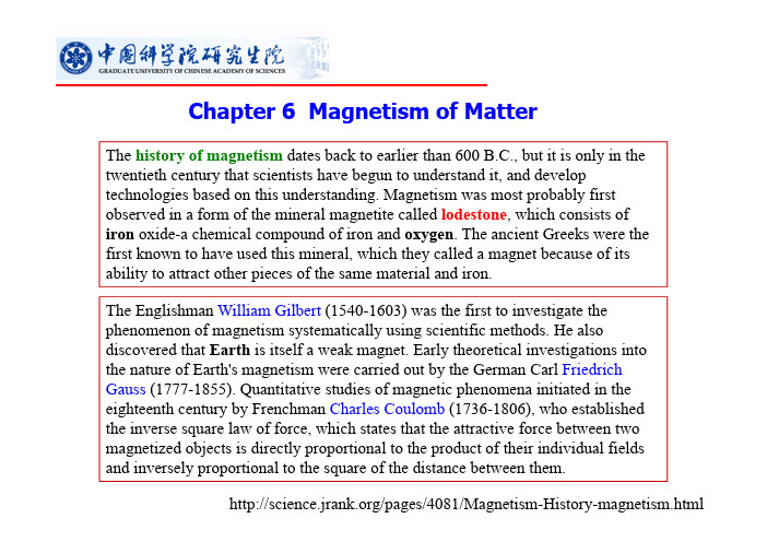
Chapter 6 Magnetism of MatterThe history of magnetism dates back to earlier than 600 B.C., but it is only in the twentieth century that scientists have begun to understand it, and develop technologies based on this understanding. Magnetism was most probably first observed in a form of the mineral magnetite called lodestone, which consists of iron oxide-a chemical compound of iron and oxygen. The ancient Greeks were the first known to have used this mineral, which they called a magnet because of its ability to attract other pieces of the same material and iron.The Englishman William Gilbert(1540-1603) was the first to investigate the phenomenon of magnetism systematically using scientific methods. He also discovered that Earth is itself a weak magnet. Early theoretical investigations into the nature of Earth's magnetism were carried out by the German Carl Friedrich Gauss(1777-1855). Quantitative studies of magnetic phenomena initiated in the eighteenth century by Frenchman Charles Coulomb(1736-1806), who established the inverse square law of force, which states that the attractive force between two magnetized objects is directly proportional to the product of their individual fields and inversely proportional to the square of the distance between them.Danish physicist Hans Christian Oersted(1777-1851) first suggested a link between electricity and magnetism. Experiments involving the effects of magnetic and electric fields on one another were then conducted by Frenchman Andre Marie Ampere(1775-1836) and Englishman Michael Faraday(1791-1869), but it was the Scotsman, James Clerk Maxwell(1831-1879), who provided the theoretical foundation to the physics of electromagnetism in the nineteenth century by showing that electricity and magnetism represent different aspects of the same fundamental force field. Then, in the late 1960s American Steven Weinberg(1933-) and Pakistani Abdus Salam(1926-96), performed yet another act of theoretical synthesis of the fundamental forces by showing that electromagnetism is one part of the electroweak force. The modern understanding of magnetic phenomena in condensed matter originates from the work of two Frenchmen: Pierre Curie(1859-1906), the husband and scientific collaborator of Madame Marie Curie(1867-1934), and Pierre Weiss(1865-1940). Curie examined the effect of temperature on magnetic materials and observed that magnetism disappeared suddenly above a certain critical temperature in materials like iron. Weiss proposed a theory of magnetism based on an internal molecular field proportional to the average magnetization that spontaneously align the electronic micromagnets in magnetic matter. The present day understanding of magnetism based on the theory of the motion and interactions of electrons in atoms (called quantum electrodynamics) stems from the work and theoretical models of two Germans, Ernest Ising and Werner Heisenberg (1901-1976). Werner Heisenberg was also one of the founding fathers of modern quantum mechanics.Magnetic CompassThe magnetic compass is an old Chinese invention, probably first made in China during the Qin dynasty (221-206 B.C.). Chinese fortune tellers used lodestonesto construct their fortune telling boards.Magnetized NeedlesMagnetized needles used as direction pointers instead of the spoon-shaped lodestones appeared in the 8th century AD, again in China, and between 850 and 1050 they seemto have become common as navigational devices on ships. Compass as a Navigational AidThe first person recorded to have used the compass as a navigational aid was Zheng He (1371-1435), from the Yunnan province in China, who made seven ocean voyages between 1405 and 1433.有关固体磁性的基本概念和规律在上个世纪电磁学的发展史中就开始建立了。
凝聚态物理相关诺贝尔奖Word版
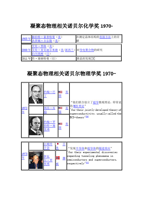
凝聚态物理相关诺贝尔化学奖1970-凝聚态物理相关诺贝尔物理学奖1970-约翰·巴丁美国美国约翰·罗伯特·施里弗美国日本“发现"for their experimental discoveriesregarding tunneling phenomena insemiconductors and superconductors,respectively"挪威英国“他理论上预测出通过隧道势垒的超电流的性质,特别是那些通常被称为象”"for his theoretical predictions of the properties of a supercurrent through a tunnel barrier, in particular those phenomena which are generally known as the Josephson effect"美国英国美国年彼得·列昂尼多维奇·卡皮苏联美国“对与相转变有关的临界现象理论的贡献”"for his theory for critical phenomena inconnection with phase transitions"克劳斯·冯·克利青德国“发现"for the discovery of thequantized Hall effect"德国德国瑞士约翰内斯·贝德诺尔茨德国卡尔·米勒瑞士法国美国美国美国若雷斯·阿尔费罗夫俄罗斯“发展了用于高速电子学和半导体异质结构"for developing semiconductorheterostructures used in high-speed-and optoelectronics"德国美国“在发明"for his part in the invention of theintegrated circuit"美国“在碱性原子稀薄气体的聚态质的早期基础性研究”"for the achievement of Bose-Einsteincondensation in dilute gases of alkaliatoms,of美国德国美国俄罗斯“对性贡献”"for pioneering contributions to thesuperfluids"俄罗斯英国美国法国德国英国美国[110]美国美国荷兰俄罗斯“在二维"for groundbreaking experiments regarding the two-dimensional material graphene"康斯坦丁·诺沃肖洛夫英国俄罗斯(注:可编辑下载,若有不当之处,请指正,谢谢!)。
基于磁屏蔽设计的磁吻合环建立大鼠胃旁路手术的实验研究
19FEATURES中国医疗设备 2021年第36卷 05期 V OL.36 No.05引言胃肠道吻合是重建消化道连续性的重要方法。
胃旁路手术通过对消化道进行改道,是经典的减重代谢手术方式[1]。
有关胃旁路手术改变机体代谢功能的机制虽有大量研究但仍未明确。
SD 大鼠是研究代谢性疾病的常用动物模型,但大鼠胃肠道较细,利用手工缝线对大鼠进行胃肠道吻合重建制备动物模型学习曲线较长,模型制备成功率较低[2]。
套管法[3]、激光焊接法[4]用于肠道吻合已有报道,但技术尚不成熟。
基于磁屏蔽设计的磁吻合环建立大鼠胃旁路手术的实验研究张苗苗1a,1b ,李恒1b,2,吝怡1b,2,魏欣怡1b,2,李美豫1b,2,刘俊杰1b,2,吕毅1a,1b ,严小鹏1a,1b1. 西安交通大学第一附属医院 a. 肝胆外科;b. 精准外科与再生医学国家地方联合工程研究中心,陕西 西安 710061;2. 西安交通大学 启德书院,陕西 西安 710061[摘 要] 目的 探讨基于磁屏蔽理论设计的磁吻合环用于大鼠胃旁路手术模型制备的可行性。
方法 根据磁屏蔽理论自行设计加工了适用于大鼠胃肠道吻合重建的坡莫合金外壳与钕铁硼内核组成的壳核结构磁吻合环。
以12只SD 大鼠为动物模型,开腹后在屈氏韧带远端16 cm 离断空肠,利用磁屏蔽结构的磁吻合环按照胃旁路手术方式依次完成胃肠吻合、肠肠吻合。
术后行正侧位片观察磁体位置、记录磁体排出时间,观察动物术后存活情况。
结果 12只SD 大鼠,除1只因麻醉意外死亡外,其余11只大鼠均顺利完成了磁吻合胃肠旁路手术,手术操作顺利,手术时间(49.73±6.34)min 。
术后动物存活良好,所有磁体均经消化道顺利排出,排出时间(9.14±1.89)d ,术后大鼠均存活良好。
结论 基于磁屏蔽理论设计的壳核结构的磁吻合环可有效避免狭小空间内多个磁体间的非计划相吸,可用于大鼠胃旁路术动物模型制备,具有操作简单、成功率高等优点。
一维磁性原子链系统中的Majorana费米子态

一维磁性原子链系统中的Majorana费米子态杨双波【摘要】对处于螺旋形磁场及横向均匀磁场的一维磁性原子链模型,在平均场近似下通过自洽地求解Bogoliubov-de-Genes方程我们计算了系统的能谱.我们发现在一定参数值的范围内能谱随螺旋形磁场振幅值演化呈现能量为零的Majorana 费米子态.我们计算了局域态密度发现对Majorana费米子其态密度的峰值出现在链的两端(或中点)位置.我们计算了波函数其空间分布,发现它与局域态密度的结果一致.%For a model of one dimensional magnetic atomic chain in both a helical magnetic field and a transverse uniform magnetic field,we calculate its energy spectrum by solving Bogoliubov-de-Genes equation selfconsistently in the mean field approximation. We find that for a certain parameter setting,energy spectrum evolving with amplitude of helical magnetic field,appears Majorana fermion eigenstates. We calculate local density of states,and find that the local density of states for Majorana fermion shows peaks at the both ends(or at middle)of the magnetic atomic chain. We calculate wave function,and its spatial distribution agrees with local density of states.【期刊名称】《南京师大学报(自然科学版)》【年(卷),期】2017(040)003【总页数】8页(P110-117)【关键词】Majorana费米子;磁性原子链;BdG方程;局域态密度【作者】杨双波【作者单位】南京师范大学物理科学与技术学院,江苏省大规模复杂系统数值模拟重点实验室,江苏南京210023【正文语种】中文【中图分类】O413.1Majorana fermion[1] which is a particle of the same as its own antiparticle,has been attracting great attention. Firstly,because of Majorana fermion being connected with topological phase concept,secondly because of its topological character,it provides a platform of potential application in topological quantum computing and quantum storing[2-4]. So experimentally and theoretically search for physical system of Majorana fermion has been a very hot research topic. The purpose of all these researches is to generate a topological superconductor,so that the Majorana fermion appears as a single excitation at the boundary. Recently,Majorana fermion has been studied for a model of an atomic chain in a helical magnetic field in close proximity to a s-wave superconductor[5-7],and the result shows that at a certain parameter setting,the Majorana fermion is localized at the both end of the magnetic atomic chain. This is a spatially uniform system,after a gauge transformation,the Hamiltonian of the system will become an invariant form for space displacement. In this paper we modified this system by adding a new Zeeman term in the original Hamiltonian,which correspondsto a uniform magnetic field h perpendicular to the atomic chain being applied to the original system. Because of the new Zeeman term,the system is nonuniform spatially,we will study the structure of the Majorana fermion for the system of h≠0.In this paper,we get the system eigenenergies and eigenvectors by numerically solving BdG equation,and then we study the birth and the localization in space of the Majorana fermion by calculating the spatially resolved local density of states and wave function. The structure of the paper is as the following,the Model and theory is in section 1,the result of numerical calculation and discussion is in section 2,the summary of the paper is in section 3.Consider a N-atom atomic chain in a helical magnetic filed or magnetic structure. The magnetic filed at site n is =B0(cosnθ+sinnθ),where θ is the angle made by the magnetic fields at the adjacent sites of the atomic chain,the whole atomic chain is in proximity to the surface of a s-wave superconductor,and in the transverse direction of the atomic chain a uniform magnetic field h is applied. The Hamiltonian of this magnetic atomic chain in mean field approximation is given byH=tx(cn+1α+h.c.)-μcnα+(cnβ+Δ(n)(+h.c.)+h(σz)ααcnα,where tx is the jumping amplitude for electron between two adjacent sites,μ is chemical potential,Δ(n)is the superconductor pairing potential or order parameter at sit n,h is the weak uniform magnetic field for tuning system energy spectrum. or cnα is the operator to creat or annihilate an electron of spin α respectively at site n, is pauli matrix vec tor,and h.c. standfor complex conjugate. By introducing Nambu spinor representationψi=(ci↑,ci↓,,-)T,then Hamiltonian(1)can be written as BdG form,i.e.H=Hijψj,where Hij is the BdG Hamiltonian at site i,which can be written as where Kij=tx(δi+1,j+δi-1,j)-μδij,γij=(h-B0cosiθ)δij. This is a 4N×4N matrix,whose energy eigenvalue εn and eigenfunctionψn(i)=(un(↑,i),un(↓,i),vn(↓,i),vn(↑,i))T, for i=1,2,…,N,is determined by eigenvalue equationand boundary condition. In mean field approximation the order parameter at site i takes the form[8]and the mean number of electron at site i iswhere fn=1/(1+eεn/kBT) is the Fermi distribution,T is temperature in Kelvin. The total number of electron isincluding spin up and spin down electrons. To determine eigenenergy,eigenfunction,order parameter,we need to selfconsistently solve eigenvalue equation(3)with(4)-(6). In this paper,we deal with the case of temperature T=0,then the order parameter and the mean number of electron in site i are given bySpecial case:h=0 and Δ(i)=Δ0,a constant. The Hamiltonian in(1)can be transformed into spatially unform form by a gauge transformation. The topologically nontrivial region of the parameter set is given bywhere Majorana fermion corresponds to εn=0. As |h|≠0,Hamiltonian in(1)is nonuniform in space,and the nontrivial region of parameter set can not be obtained analytically.In this paper we deal with open boundary condition with and without themiddle magnetic domain wall,and at the magnetic domain wall we replace θ by -θ. We have also studied under the periodic boundary condition,and found the result has no significant changes.We first study the character of the Majorana fermion as the order parameter Δ and chemical potential μ are constants,then we study the influence of nonuniform Δ(i)on the result of Majorana fermion by doing selfconsistent calculation. In calculation,we choose the number of site N for the atomic chain according to the angle θ,so that the magnetic field at the both ends of the atomic chain points to the same direction.2.1 Energy Spectrum and Wave FunctionsFor a one-dimensional magnetic atomic chain with magnetic domain wall in the middle,the parameter set is chosen asΔ0=1.0,tx=1.0,μ=2.5,h=0.1,θ=π/2,and length of the chain is chosen asN=81 sites. For every value of B0 in the interval[1.0,4.0],we diagonalize the 4N×4N BdG Hamiltonian matrix(2),we get 4N energy eigenvalues and 4N eigenvectors. In open boundary condition,the energy spectrum is shown in Fig.1. For B0 in the interval[1.486 6,3.996 8],we can see that thereexists eigenstates whose eigenenergy εn=0,and these eigenstates are Majorana fermions. The interval for the existense of Majorana fermion in the case of h=0.1 is very close to the interval[1.476,4.039]calculatedfrom(9)for the h=0 case. For Majorana fer mion at B0=2.1,εn=0,shown in red dot in Fig.1,we calculate its wave functionun(↑,i),un(↓,i),vn(↑,i),vn(↓,i),the result is shown in Fig.2(a-d). We can see that the amplitude of the wave function concentrates on the both ends and themiddle of the atomic chain. In Fig.3,we show wave function for the same magnetic atomic chain without magnetic domain wall in the middle,the amplitude of the wave function concentrates on both ends of the magnetic atomic chain. This is similar to the previous result for the 1-dimensional magnetic atomic chain without uniform magnetic field,h=0.2.2 Local Density of States and Total Density of StatesIn this subsection,we study the space distribution of density ofstates(DOS),which is called local density of states(LDOS)and is defined as ρ(ε,i)is a function of energy and space position,and the total density of states(TDOS)can be written as,i.e.,the arithmetic mean of local density of states,a function of energy only. In numerical calculation,we replace δ by a Lorentz function. Fo r parameter setting h=0.1,tx=1.0,Δ=1.0,μ=2.5,θ=π/2,N=81,and B0=2.1,the local density of states for a Majorana fermion and the mean number of electrons on each site are shown in Fig.4(a-d)for the magnetic atomic chain with magnetic domain wall in the middle. Fig.4(a)shows the local density of states ρ(ε,i)in a 3D-plot;Fig.4(b)shows the local density of states ρ(ε,i)in a 2D contour plot;Fig.4(c)shows the local density of states for Majorana fermion ρ(ε=0,i);Fig.4(d)shows the mean number of electron on each si te of atomic chain<n(i)>. We can see from the Fig.4 that the Majorana fermion is localized at two ends and middle for the magnetic atomic chain with magnetic domain wall in the middle. The mean number of electrons on each site of the atomic chain is around 1.5. In Fig.5(a-d)we show theresult for the same magnetic atomic chain without magnetic domain wall in the middle,then we see density of states for Majorana fermion is peaked only at both ends of the magnetic atomic chain.2.3 The Self-consistent ResultAs the order parameter Δ(i)is space position i dependent,we calculate the energy spectrum and local density of states by selfconsistently solving the eigenvalue equation(3)with equations(7)and(8). For parameter seth=0.1,tx=1.0,μ=2.5,U0=4.0,θ=π/2,N=81,the selfconsistently calculated energy spectrum is shown in Fig.6,the Majorana fermion region can be seen,is still there,but the interval is shorten. The local density of states and mean numbers of electron on each site for Majorana fermion at B0=1.57 are shown in Fig.7(a-d)and Fig.9(a-d). By comparison with Fig.4(a-d),we find the main characters are same,but peak position for selfconsistent result moved inside a little bit. We calculate the selfconsistent wave function for Majorana fermion,and the results are shown in Fig.8(a-d)and Fig.10(a-d). The amplitude is significiently large at both ends for magnetic atomic chain without magnetic domain wall,and significiently large at both ends and middle for a magnetic chain with magnetic domain wall in the middle. This agrees with the result of local density of states.In mean field approximation,and by numerically solving Bogoliubov-de-Genes(BdG)equation,this paper studies the birth,and the localization in space of the Majorana fermion in a one dimensional atomic chain in helical magnetic field,and a uniform magnetic field h which is perpendicular to the atomic chain. Studies find that at a certain parameter setting,theevolution of the energy spectrum with helical magnetic field amplitude B0 appears the zero energy eigenstates,which corresponding to the Majorana fermion. We calculate the local density of states,and find that the local density of states for the Majorana fermion has two peaks on the both end of the magnetic atomic chain. When a magnetic domain wall is applied at the middle of the maqgnetic atomic chain,the Majorana fermion shows peaks at both ends and the middle of the magnetic chain. As the order parameter is a function of space coordinate,we do selfconsistent calculation,and find that by comparing with the result of nonselfconsistent calculation,the energy spectrum and the shape of the local density of states are changed a little bit,but the main character does not change. [1] MAJORANA E. Symmetric theory of electron and positrons[J]. Nuovo Cimento,1937,14(1):171-181.[2] WILCZEK F. Majorana returns[J]. Nat Phys,2009,5(9):614-618.[3] NAYAK C,SIMON S H,STERN A,et al. Non-Abelian anyons and topological quantum computation[J]. Rev Mod Phys,2008,80(3):1 083-1 159.[4] ALICEA J. New directions in the persuit of Majorana fermions in solid state system[J]. Rep Prog Phys,2012,75(7):076501-1-36.[5] NADJ-PERGE S,DROZDOV I K,BERNEVIG B A,et al. Proposal for realizing Majorana fermions in chain of magnetic atoms on a superconductor [J]. Phys Rev B,2013,88(2):020407-1-5(R).[6] PÖYHÖNEN K,WESTSTRÖM A,RÖNTYNEN J,et al. Majorana state in helical shiba chain and ladders[J]. Phys Rev B,2014,89(11):115109-1-7.[7] VAZIFEH M M,FRANZ M. Self-organized topological state with Majorana fermions[J]. Phys Rev Lett,2013,111(20):206802-1-5.[8] SACRAMENTO P D,DUGAEV V K,VIEIRA V R. Magnetic impurities in a superconductors:effect of domainwall and interference[J]. Phys RevB,2007,76(1):014512-1-21.[9] EBISU H,YADA K,KASAI H,et al. Odd frequency pairing in topological superconductivity in a one dimensional magnetic chain[J]. Phys RevB,2015,91(5):054518-1-15.【相关文献】Received data:2016-11-17.Corresponding author:Yang Shuangbo,professor,majored in nonlinear physics and low dimensionalsystem.E-mail:*********************.cndoi:10.3969/j.issn.1001-4616.2017.03.016CLC number:O413.1 Document codeA Article ID1001-4616(2017)03-0110-08。
FDTD Solutions资料集锦专题资料(四)

defined local structures.
Numerical study of natural convection in porous media (metals)
using Lattice Boltzmann Method (LBM).pdf 自然对流多孔介质(金属)用晶格玻尔兹曼方法加快的数值研究
The use of latent heat storage, microencapsulated phase change
materials (MEPCMs), is one of the most efficient ways of storing thermal energy and it has received a growing attention in the past
评价的线性和非线性光学聚合物的二次电光系数衰减全反射技术
The impact of local resonance on the enhanced transmission and dispersion of surface resonances.pdf 局部表面共振对传输和分散增强的影响
We investigate the enhanced transmission through the square array
decade.
Plasmonic Nanoclusters Near Field Properties of the Fano
Resonance Interrogated with SERS.pdf 近场法诺共振制备电浆的性能研究
Review on thermal transport in high porosity cellular metal
- 1、下载文档前请自行甄别文档内容的完整性,平台不提供额外的编辑、内容补充、找答案等附加服务。
- 2、"仅部分预览"的文档,不可在线预览部分如存在完整性等问题,可反馈申请退款(可完整预览的文档不适用该条件!)。
- 3、如文档侵犯您的权益,请联系客服反馈,我们会尽快为您处理(人工客服工作时间:9:00-18:30)。
PACS number(s): 75.10.-b, 71.28.+d, 71.45.-d
1
Introduction
In the theory of strongly correlated itinerant electron systems two topics are of continued interest, namely (i) the localized–itinerant complementarity and (ii) the competition between magnetic long–range order (LRO) and short–range order (SRO). In particular, the concept of magnetic SRO and its interrelation to itinerant properties was investigated in the context of both narrow–band magnetism of transition metals and their compounds [1–6] and of the unconventional magnetic behaviour of high–Tc copper oxides [7–12]. In the cuprates, neutron scattering [13] and nuclear magnetic resonance experiments [14] reveal pronounced antiferromagnetic spin correlations within the CuO2 planes which persist even in the superconducting phase. Moreover, measurements of the spin susceptibility χ(T, δ) in the normal metallic state of La2−δ Srδ CuO4 (LSCO) [15, 16] show a maximum in the doping dependence as well as (for δ< ∼ 0.21) in the temperature dependence and give further evidence for strong SRO effects at low temperatures, where the SRO decreases with increasing doping and temperature. Thus the experiments on cuprates bring out the importance of electron correlations as compared with the situation in traditional band magnetism, and therefore yield a new challenge for a microscopic theory of SRO in itinerant electron systems. Such a theory has to provide a self–consistent description of strong SRO (in the absence of LRO) down to zero temperature. The previous theoretical approaches to the problem of SRO in transition metals and cuprates are mostly based on Hubbard–type models [1, 2, 4–6, 8–12, 17]. For example, to explain the normal–state susceptibility of LSCO in terms of SRO, the three–band Hubbard model was used [9]. In connection with the study of SRO some general problems have gained a renewed interest, such as the stability of various magnetic LRO phases against paraphases with and without SRO as well as the question of phase separation in strong correlation models [18, 12]. From the methodical point of view, the SRO theories for itinerant systems are preferentially formulated within functional–integral representations of the one–band Hubbard model using the static approximation. Thereby, various Hubbard–Stratonovich two–field methods, often combined with the single–site coherent potential approximation (CPA) [1, 2, 5, 6, 8] and,
Theory of magnetic short–range order for itinerant el/9609014v1 2 Sep 1996
U. Trapper(1) , D. Ihle(1) and H. Fehske(2)
(1)
Institut f¨ ur Theoretische Physik, Universit¨ at Leipzig, D–04109 Leipzig, Germany
(2)
Physikalisches Institut, Universit¨ at Bayreuth, D–95440 Bayreuth, Germany
February 1, 2008
Abstract On the basis of the one–band t–t′ –Hubbard model a self–consistent renormalization theory of magnetic short–range order (SRO) in the paramagnetic phase is presented combining the four–field slave–boson functional–integral scheme with the cluster variational method. Contrary to previous SRO approaches the SRO is incorporated at the saddle–point and pair–approximation levels. A detailed numerical evaluation of the theory is performed at zero temperature, where both the hole– and electron–doped cases as well as band–structure effects are studied. The ground–state phase diagram shows the suppression of magnetic long–range order in favour of a paramagnetic phase with antiferromagnetic SRO in a wide doping region. In this phase the uniform static spin susceptibility increases upon doping up to the transition to the Pauli paraphase. Comparing the theory with experiments on high–Tc cuprates a good agreement is found.
2
in the context of high–Tc ’s, the scalar four–field slave–boson approach [19, 9, 12] where employed. Those theories are designed to describe the formation and ordering of local magnetic moments in an itinerant system on a time scale large compared to the electron hopping time. In the mode–mode coupling theory of spin fluctuations (SF) by Moriya et al. [1, 2] interpolating between the weakly magnetic (local SF in q –space) and local moment (local SF in real space) limits, the SRO is reflected in the spatial correlation of thermal SF (with an amplitude increasing with temperature) and is appreciable even above the Curie temperature. Starting from the local moment limit and using the two–vector–field Hubbard–Stratonovich/CPA approach, the SRO is taken into account by an expansion in pairwise terms (within the bilinear approximation) around the single–site CPA saddle–point. The lack of self–consistency in this approach may be justified when the SRO is weak. Note that, at T = 0, the theory by Moriya et al. [1, 2] reduces to the Hartree–Fock approximation in both the weak– and strong–coupling limits, and the SRO is lost. The neglect of important correlations at zero temperature may be the reason for the absence of a maximum in the calculated spin susceptibility. Contrary, the phenomenological version of the interpolation theory given in Ref. [2] incorporates the SRO at the saddle point, and in the weakly magnetic limit the results of the classical approximation to the self–consistent renormalization theory of SF are recovered. In the local–band theory of ferromagnetism [3, 4], where the fluctuations of the local magnetizations with a fixed amplitude are considered to be local in q –space, the SRO is described by an expansion around the Stoner saddle point [4] and turns out to be strong near the Curie temperature. As in Ref. [1], the SRO–induced renormalization of the saddle point is disregarded. The non–self consistency is also inherent in the SRO theories taking the SF to be local in real space and employing various cluster methods [5, 6, 8, 9]. For example, in the approaches of Refs. [6] and [9] resulting in an effective Ising free–energy functional, where the exchange energy is evaluated beyond the bilinear approximation used in Ref. [1] and is nearly independent on temperature, the SRO is treated by an expansion around the single–site CPA saddle–point and by the Bethe–Peierls approximation [20].