MCM美国大学生数学建模竞赛模板-摘要
MCM美国大学生数学建模竞赛模板-公式
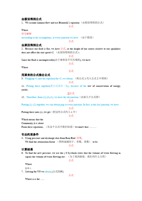
由假设得到公式1.We assume laminar flow and use Bernoulli’s equation:(由假设得到的公式)公式Where符号解释According to the assumptions, at every junction we have(由于假设)公式由原因得到公式2.Because our field is flat, we have公式, so the height of our source relative to our sprinklers does not affect the exit speed v2 (由原因得到的公式);公式Since the fluid is incompressible(由于液体是不可压缩的), we have公式Where公式用原来的公式推出公式3.Plugging v1 into the equation for v2 ,we obtain(将公式1代入公式2中得到)公式11.Putting these together(把公式放在一起), because of the law of conservation of energy, yields:[]公式12.Therefore, from (2),(3),(5), we have the ith junction(由前几个公式得)公式Putting (1)-(5) together, we can obtain pup at every junction. In fact, at the last junction, we have公式Putting these into (1) ,we get(把这些公式代入1中)公式Which means that theCommonly, h is aboutFrom these equations, (从这个公式中我们知道)we know that ………引出约束条件4.Using pressure and discharge data from Rain Bird 结果,We find the attenuation factor (得到衰减因子,常数,系数)to be公式计算结果6.To find the new pressure ,we use the ( 0 0),which states that the volume of water flowing in equals the volume of water flowing out : (为了找到新值,我们用什么方程)公式Where() is ;;7.Solving for VN we obtain (公式的解)公式Where n is the …..8.We have the following differential equations for speeds in the x- and y- directions:公式Whose solutions are (解)公式9.We use the following initial conditions ( 使用初值) to determine the drag constant:公式根据原有公式10.We apply the law of conservation of energy(根据能量守恒定律). The work done by the forces is公式The decrease in potential energy is (势能的减少)公式The increase in kinetic energy is (动能的增加)公式Drug acts directly against velocity, so the acceleration vector from drag can be found Newton’s law F=ma as : (牛顿第二定律)Where a is the acceleration vector and m is massUsing the Newton’s Second Law, we have that F/m=a and公式So that公式Setting the two expressions for t1/t2 equal and cross-multiplying gives公式22.We approximate the binomial distribution of contenders with a normal distribution:公式Where x is the cumulative distribution function of the standard normal distribution. Clearing denominators and solving the resulting quadratic in B gives公式As an analytic approximation to . for k=1, we get B=c26.Integrating, (使结合)we get PVT=constant, where公式The main composition of the air is nitrogen and oxygen, so i=5 and r=1.4, so23.According to First Law of Thermodynamics, we get公式Where ( ) . we also then have公式Where P is the pressure of the gas and V is the volume. We put them into the Ideal Gas Internal Formula:公式Where对公式变形13.Define A=nlw to be the ( )(定义); rearranging (1) produces (将公式变形得到)公式We maximize E for each layer, subject to the constraint (2). The calculations are easier if we minimize 1/E.(为了得到最大值,求他倒数的最小值)Neglecting constant factors (忽略常数), we minimize公式使服从约束条件14.Subject to the constraint (使服从约束条件)公式Where B is constant defined in (2). However, as long as we are obeying this constraint, we can write (根据约束条件我们得到)公式And thus f depends only on h , the function f is minimized at (求最小值)公式At this value of h, the constraint reduces to公式结果说明15.This implies(暗示)that the harmonic mean of l and w should be公式So , in the optimal situation. ………5.This value shows very little loss due to friction.(结果说明)The escape speed with friction is公式16.We use a similar process to find the position of the droplet, resulting in公式With t=0.0001 s, error from the approximation is virtually zero.17.We calculated its trajectory(轨道) using公式18.For that case, using the same expansion for e as above,公式19.Solving for t and equating it to the earlier expression for t, we get公式20.Recalling that in this equality only n is a function of f, we substitute for n and solve for f. the result is公式As v=…, this equation becomes singular (单数的).由语句得到公式21.The revenue generated by the flight is公式24.Then we have公式We differentiate the ideal-gas state equation公式Getting公式25.We eliminate dT from the last two equations to get (排除因素得到)公式22.We fist examine the path that the motorcycle follows. Taking the air resistance into account, we get two differential equations公式Where P is the relative pressure, we must first find the speed v1 of water at our source: (找初值)公式自己根据计算所画的图:1、为了…….(目的),我们作了…….图。
2014年美国大学生数学建模MCM-B题O奖论文
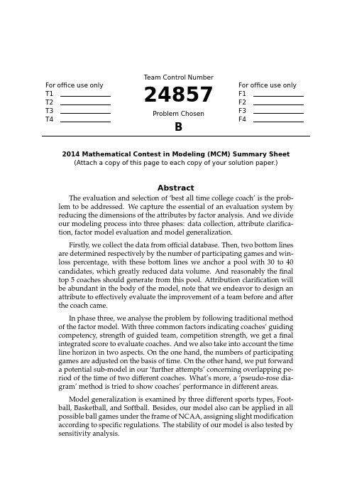
For office use only T1T2T3T4T eam Control Number24857Problem ChosenBFor office use onlyF1F2F3F42014Mathematical Contest in Modeling(MCM)Summary Sheet (Attach a copy of this page to each copy of your solution paper.)AbstractThe evaluation and selection of‘best all time college coach’is the prob-lem to be addressed.We capture the essential of an evaluation system by reducing the dimensions of the attributes by factor analysis.And we divide our modeling process into three phases:data collection,attribute clarifica-tion,factor model evaluation and model generalization.Firstly,we collect the data from official database.Then,two bottom lines are determined respectively by the number of participating games and win-loss percentage,with these bottom lines we anchor a pool with30to40 candidates,which greatly reduced data volume.And reasonably thefinal top5coaches should generate from this pool.Attribution clarification will be abundant in the body of the model,note that we endeavor to design an attribute to effectively evaluate the improvement of a team before and after the coach came.In phase three,we analyse the problem by following traditional method of the factor model.With three common factors indicating coaches’guiding competency,strength of guided team,competition strength,we get afinal integrated score to evaluate coaches.And we also take into account the time line horizon in two aspects.On the one hand,the numbers of participating games are adjusted on the basis of time.On the other hand,we put forward a potential sub-model in our‘further attempts’concerning overlapping pe-riod of the time of two different coaches.What’s more,a‘pseudo-rose dia-gram’method is tried to show coaches’performance in different areas.Model generalization is examined by three different sports types,Foot-ball,Basketball,and Softball.Besides,our model also can be applied in all possible ball games under the frame of NCAA,assigning slight modification according to specific regulations.The stability of our model is also tested by sensitivity analysis.Who’s who in College Coaching Legends—–A generalized Factor Analysis approach2Contents1Introduction41.1Restatement of the problem (4)1.2NCAA Background and its coaches (4)1.3Previous models (4)2Assumptions5 3Analysis of the Problem5 4Thefirst round of sample selection6 5Attributes for evaluating coaches86Factor analysis model106.1A brief introduction to factor analysis (10)6.2Steps of Factor analysis by SPSS (12)6.3Result of the model (14)7Model generalization15 8Sensitivity analysis189Strength and Weaknesses199.1Strengths (19)9.2Weaknesses (19)10Further attempts20 Appendices22 Appendix A An article for Sports Illustrated221Introduction1.1Restatement of the problemThe‘best all time college coach’is to be selected by Sports Illustrated,a magazine for sports enthusiasts.This is an open-ended problem—-no limitation in method of performance appraisal,gender,or sports types.The following research points should be noted:•whether the time line horizon that we use in our analysis make a difference;•the metrics for assessment are to be articulated;•discuss how the model can be applied in general across both genders and all possible sports;•we need to present our model’s Top5coaches in each of3different sports.1.2NCAA Background and its coachesNational Collegiate Athletic Association(NCAA),an association of1281institution-s,conferences,organizations,and individuals that organizes the athletic programs of many colleges and universities in the United States and Canada.1In our model,only coaches in NCAA are considered and ranked.So,why evaluate the Coaching performance?As the identity of a college football program is shaped by its head coach.Given their impacts,it’s no wonder high profile athletic departments are shelling out millions of dollars per season for the services of coaches.Nick Saban’s2013total pay was$5,395,852and in the same year Coach K earned$7,233,976in total23.Indeed,every athletic director wants to hire the next legendary coach.1.3Previous modelsTraditionally,evaluation in athletics has been based on the single criterion of wins and losses.Years later,in order to reasonably evaluate coaches,many reseachers have implemented the coaching evaluation model.Such as7criteria proposed by Adams:[1] (1)the coach in the profession,(2)knowledge of and practice of medical aspects of coaching,(3)the coach as a person,(4)the coach as an organizer and administrator,(5) knowledge of the sport,(6)public relations,and(7)application of kinesiological and physiological principles.1Wikipedia:/wiki/National_Collegiate_Athletic_ Association#NCAA_sponsored_sports2USAToday:/sports/college/salaries/ncaaf/coach/ 3USAToday:/sports/college/salaries/ncaab/coach/Such models relatively focused more on some subjective and difficult-to-quantify attributes to evaluate coaches,which is quite hard for sports fans to judge coaches. Therefore,we established an objective and quantified model to make a list of‘best all time college coach’.2Assumptions•The sample for our model is restricted within the scale of NCAA sports.That is to say,the coaches we discuss refers to those service for NCAA alone;•We do not take into account the talent born varying from one player to another, in this case,we mean the teams’wins or losses purely associate with the coach;•The difference of games between different Divisions in NCAA is ignored;•Take no account of the errors/amendments of the NCAA game records.3Analysis of the ProblemOur main goal is to build and analyze a mathematical model to choose the‘best all time college coach’for the previous century,i.e.from1913to2013.Objectively,it requires numerous attributes to judge and specify whether a coach is‘the best’,while many of the indicators are deemed hard to quantify.However,to put it in thefirst place, we consider a‘best coach’is,and supposed to be in line with several basic condition-s,which are the prerequisites.Those prerequisites incorporate attributes such as the number of games the coach has participated ever and the win-loss percentage of the total.For instance,under the conditions that either the number of participating games is below100,or the win-loss percentage is less than0.5,we assume this coach cannot be credited as the‘best’,ignoring his/her other facets.Therefore,an attempt was made to screen out the coaches we want,thus to narrow the range in ourfirst stage.At the very beginning,we ignore those whose guiding ses-sions or win-loss percentage is less than a certain level,and then we determine a can-didate pool for‘the best coach’of30-40in scale,according to merely two indicators—-participating games and win-loss percentage.It should be reasonably reliable to draw the top5best coaches from this candidate pool,regardless of any other aspects.One point worth mentioning is that,we take time line horizon as one of the inputs because the number of participating games is changing all the time in the previous century.Hence,it would be unfair to treat this problem by using absolute values, especially for those coaches who lived in the earlier ages when sports were less popular and games were sparse comparatively.4Thefirst round of sample selectionCollege Football is thefirst item in our research.We obtain data concerning all possible coaches since it was initiated,of which the coaches’tenures,participating games and win-loss percentage etc.are included.As a result,we get a sample of2053in scale.Thefirst10candidates’respective information is as below:Table1:Thefirst10candidates’information,here Pct means win-loss percentageCoach From To Years Games Wins Losses Ties PctEli Abbott19021902184400.5Earl Abell19281930328141220.536Earl Able1923192421810620.611 George Adams1890189233634200.944Hobbs Adams1940194632742120.185Steve Addazio20112013337201700.541Alex Agase1964197613135508320.378Phil Ahwesh19491949193600.333Jim Aiken19461950550282200.56Fred Akers19751990161861087530.589 ...........................Firstly,we employ Excel to rule out those who begun their coaching career earlier than1913.Next,considering the impact of time line horizon mentioned in the problem statement,we import our raw data into MATLAB,with an attempt to calculate the coaches’average games every year versus time,as delineated in the Figure1below.Figure1:Diagram of the coaches’average sessions every year versus time It can be drawn from thefigure above,clearly,that the number of each coach’s average games is related with the participating time.With the passing of time and the increasing popularity of sports,coaches’participating games yearly ascends from8to 12or so,that is,the maximum exceed the minimum for50%around.To further refinethe evaluation method,we make the following adjustment for coaches’participating games,and we define it as each coach’s adjusted participating games.Gi =max(G i)G mi×G iWhere•G i is each coach’s participating games;•G im is the average participating games yearly in his/her career;and•max(G i)is the max value in previous century as coaches’average participating games yearlySubsequently,we output the adjusted data,and return it to the Excel table.Obviously,directly using all this data would cause our research a mass,and also the economy of description is hard to achieved.Logically,we propose to employ the following method to narrow the sample range.In general,the most essential attributes to evaluate a coach are his/her guiding ex-perience(which can be shown by participating games)and guiding results(shown by win-loss percentage).Fortunately,these two factors are the ones that can be quantified thus provide feasibility for our modeling.Based on our common sense and select-ed information from sports magazines and associated programs,wefind the winning coaches almost all bear the same characteristics—-at high level in both the partici-pating games and the win-loss percentage.Thus we may arbitrarily enact two bottom line for these two essential attributes,so as to nail down a pool of30to40candidates. Those who do not meet our prerequisites should not be credited as the best in any case.Logically,we expect the model to yield insight into how bottom lines are deter-mined.The matter is,sports types are varying thus the corresponding features are dif-ferent.However,it should be reasonably reliable to the sports fans and commentators’perceptual intuition.Take football as an example,win-loss percentage that exceeds0.75 should be viewed as rather high,and college football coaches of all time who meet this standard are specifically listed in Wikipedia.4Consequently,we are able tofix upon a rational pool of candidate according to those enacted bottom lines and meanwhile, may tender the conditions according to the total scale of the coaches.Still we use Football to further articulate,to determine a pool of candidates for the best coaches,wefirst plot thefigure below to present the distributions of all the coaches.From thefigure2,wefind that once the games number exceeds200or win-loss percentage exceeds0.7,the distribution of the coaches drops significantly.We can thus view this group of coaches as outstanding comparatively,meeting the prerequisites to be the best coaches.4Wikipedia:/wiki/List_of_college_football_coaches_ with_a_.750_winning_percentageFigure2:Hist of the football coaches’number of games versus and average games every year versus games and win-loss percentageHence,we nail down the bottom lines for both the games number and the win-loss percentage,that is,0.7for the former and200for the latter.And these two bottom lines are used as the measure for ourfirst round selection.After round one,merely35 coaches are qualified to remain in the pool of candidates.Since it’s thefirst round sifting,rather than direct and ultimate determination,we hence believe the subjectivity to some extent in the opt of bottom lines will not cloud thefinal results of the best coaches.5Attributes for evaluating coachesThen anchored upon the35candidate selected,we will elaborate our coach evaluation system based on8attributes.In the indicator-select process,we endeavor to examine tradeoffs among the availability for data and difficulty for data quantification.Coaches’pay,for example,though serves as the measure for coaching evaluation,the corre-sponding data are limited.Situations are similar for attributes such as the number of sportsmen the coach ever cultivated for the higher-level tournaments.Ultimately,we determine the8attributes shown in the table below:Further explanation:•Yrs:guiding years of a coach in his/her whole career•G’:Gi =max(G i)G mi×G i see it at last section•Pct:pct=wins+ties/2wins+losses+ties•SRS:a rating that takes into account average point differential and strength of schedule.The rating is denominated in points above/below average,where zeroTable2:symbols and attributessymbol attributeYrs yearsG’adjusted overall gamesPct win-lose percentageP’Adjusted percentage ratioSRS Simple Rating SystemSOS Strength of ScheduleBlp’adjusted Bowls participatedBlw’adjusted Bowls wonis the average.Note that,the bigger for this value,the stronger for the team performance.•SOS:a rating of strength of schedule.The rating is denominated in points above/below average,where zero is the average.Noted that the bigger for this value,the more powerful for the team’s rival,namely the competition is more fierce.Sports-reference provides official statistics for SRS and SOS.5•P’is a new attribute designed in our model.It is the result of Win-loss in the coach’s whole career divided by the average of win-loss percentage(weighted by the number of games in different colleges the coach ever in).We bear in mind that the function of a great coach is not merely manifested in the pure win-loss percentage of the team,it is even more crucial to consider the improvement of the team’s win-loss record with the coach’s participation,or say,the gap between‘af-ter’and‘before’period of this team.(between‘after’and‘before’the dividing line is the day the coach take office)It is because a coach who build a comparative-ly weak team into a much more competitive team would definitely receive more respect and honor from sports fans.To measure and specify this attribute,we col-lect the key official data from sports-reference,which included the independent win-loss percentage for each candidate and each college time when he/she was in the team and,the weighted average of all time win-loss percentage of all the college teams the coach ever in—-regardless of whether the coach is in the team or not.To articulate this attribute,here goes a simple physical example.Ike Armstrong (placedfirst when sorted by alphabetical order),of which the data can be ob-tained from website of sports-reference6.We can easily get the records we need, namely141wins,55losses,15ties,and0.704for win-losses percentage.Fur-ther,specific wins,losses,ties for the team he ever in(Utab college)can also be gained,respectively they are602,419,30,0.587.Consequently,the P’value of Ike Armstrong should be0.704/0.587=1.199,according to our definition.•Bowl games is a special event in thefield of Football games.In North America,a bowl game is one of a number of post-season college football games that are5sports-reference:/cfb/coaches/6sports-reference:/cfb/coaches/ike-armstrong-1.htmlprimarily played by teams from the Division I Football Bowl Subdivision.The times for one coach to eparticipate Bowl games are important indicators to eval-uate a coach.However,noted that the total number of Bowl games held each year is changing from year to year,which should be taken into consideration in the model.Other sports events such as NCAA basketball tournament is also ex-panding.For this reason,it is irrational to use the absolute value of the times for entering the Bowl games (or NCAA basketball tournament etc.)and the times for winning as the evaluation measurement.Whereas the development history and regulations for different sports items vary from one to another (actually the differentiation can be fairly large),we here are incapable to find a generalized method to eliminate this discrepancy ,instead,in-dependent method for each item provide a way out.Due to the time limitation for our research and the need of model generalization,we here only do root extract of blp and blw to debilitate the differentiation,i.e.Blp =√Blp Blw =√Blw For different sports items,we use the same attributes,except Blp’and Blw’,we may change it according to specific sports.For instance,we can use CREG (Number of regular season conference championship won)and FF (Number of NCAA Final Four appearance)to replace Blp and Blw in basketball games.With all the attributes determined,we organized data and show them in the table 3:In addition,before forward analysis there is a need to preprocess the data,owing to the diverse dimensions between these indicators.Methods for data preprocessing are a lot,here we adopt standard score (Z score)method.In statistics,the standard score is the (signed)number of standard deviations an observation or datum is above the mean.Thus,a positive standard score represents a datum above the mean,while a negative standard score represents a datum below the mean.It is a dimensionless quantity obtained by subtracting the population mean from an individual raw score and then dividing the difference by the population standard deviation.7The standard score of a raw score x is:z =x −µσIt is easy to complete this process by statistical software SPSS.6Factor analysis model 6.1A brief introduction to factor analysisFactor analysis is a statistical method used to describe variability among observed,correlated variables in terms of a potentially lower number of unobserved variables called factors.For example,it is possible that variations in four observed variables mainly reflect the variations in two unobserved variables.Factor analysis searches for 7Wikipedia:/wiki/Standard_scoreTable3:summarized data for best college football coaches’candidatesCoach From To Yrs G’Pct Blp’Blw’P’SRS SOS Ike Armstrong19251949252810.70411 1.199 4.15-4.18 Dana Bible19151946313860.7152 1.73 1.0789.88 1.48 Bernie Bierman19251950242780.71110 1.29514.36 6.29 Red Blaik19341958252940.75900 1.28213.57 2.34 Bobby Bowden19702009405230.74 5.74 4.69 1.10314.25 4.62 Frank Broyles19571976202570.7 3.162 1.18813.29 5.59 Bear Bryant19451982385080.78 5.39 3.87 1.1816.77 6.12 Fritz Crisler19301947182080.76811 1.08317.15 6.67 Bob Devaney19571972162080.806 3.16 2.65 1.25513.13 2.28 Dan Devine19551980222800.742 3.16 2.65 1.22613.61 4.69 Gilmour Dobie19161938222370.70900 1.27.66-2.09 Bobby Dodd19451966222960.713 3.613 1.18414.25 6.6 Vince Dooley19641988253250.715 4.47 2.83 1.09714.537.12 Gus Dorais19221942192320.71910 1.2296-3.21 Pat Dye19741992192400.707 3.16 2.65 1.1929.68 1.51 LaVell Edwards19722000293920.716 4.69 2.65 1.2437.66-0.66 Phillip Fulmer19922008172150.743 3.87 2.83 1.08313.42 4.95 Woody Hayes19511978283290.761 3.32 2.24 1.03117.418.09 Frank Kush19581979222710.764 2.65 2.45 1.238.21-2.07 John McKay19601975162070.7493 2.45 1.05817.298.59 Bob Neyland19261952212860.829 2.65 1.41 1.20815.53 3.17 Tom Osborne19731997253340.8365 3.46 1.18119.7 5.49 Ara Parseghian19561974192250.71 2.24 1.73 1.15317.228.86 Joe Paterno19662011465950.749 6.08 4.9 1.08914.01 5.01 Darrell Royal19541976232970.7494 2.83 1.08916.457.09 Nick Saban19902013182390.748 3.74 2.83 1.12313.41 3.86 Bo Schembechler19631989273460.775 4.12 2.24 1.10414.86 3.37 Francis Schmidt19221942212670.70800 1.1928.490.16 Steve Spurrier19872013243160.733 4.363 1.29313.53 4.64 Bob Stoops19992013152070.804 3.74 2.65 1.11716.66 4.74 Jock Sutherland19191938202550.81221 1.37613.88 1.68 Barry Switzer19731988162090.837 3.61 2.83 1.16320.08 6.63 John Vaught19471973253210.745 4.24 3.16 1.33814.7 5.26 Wallace Wade19231950243070.765 2.24 1.41 1.34913.53 3.15 Bud Wilkinson19471963172220.826 2.83 2.45 1.14717.54 4.94 such joint variations in response to unobserved latent variables.The observed vari-ables are modelled as linear combinations of the potential factors,plus‘error’terms. The information gained about the interdependencies between observed variables can be used later to reduce the set of variables in a putationally this technique is equivalent to low rank approximation of the matrix of observed variables.8 Why carry out factor analyses?If we can summarise a multitude of measure-8Wikipedia:/wiki/Factor_analysisments with a smaller number of factors without losing too much information,we have achieved some economy of description,which is one of the goals of scientific investi-gation.It is also possible that factor analysis will allow us to test theories involving variables which are hard to measure directly.Finally,at a more prosaic level,factor analysis can help us establish that sets of questionnaire items(observed variables)are in fact all measuring the same underlying factor(perhaps with varying reliability)and so can be combined to form a more reliable measure of that factor.6.2Steps of Factor analysis by SPSSFirst we import the decided datasets of8attributes into SPSS,and the results can be obtained below after the software processing.[2-3]Figure3:Table of total variance explainedFigure4:Scree PlotThefirst table and scree plot shows the eigenvalues and the amount of variance explained by each successive factor.The remaining5factors have small eigenvalues value.Once the top3factors are extracted,it adds up to84.3%,meaning a great as the explanatory ability for the original information.To reflect the quantitative analysis of the model,we obtain the following factor loading matrix,actually the loadings are in corresponding to the weight(α1,α2 (i)the set ofx i=αi1f1+αi2f2+...+αim f j+εiAnd the relative strength of the common factors and the original attribute can also be manifested.Figure5:Rotated Component MatrixThen,with Rotated Component Matrix above,wefind the common factor F1main-ly expresses four attributes they are:G,Yrs,P,SRS,and logically,we define the com-mon factor generated from those four attributes as the guiding competency of the coach;similarly,the common factor F2mainly expresses two attributes,and they are: Pct and Blp,which can be de defined as the integrated strength of the guided team; while the common factor F3,mainly expresses two attributes:SOS and Blw,which can be summarized into a‘latent attribute’named competition strength.In order to obtain the quantitative relation,we get the following Component Score Coefficient Matrix processed by SPSS.Further,the function of common factors and the original attributes is listed as bel-low:F1=0.300x1+0.312x2+0.023x3+0.256x4+0.251x5+0.060x6−0.035x7−0.053x8F2=−0.107x1−0,054x2+0.572x3+0.103x4+0.081x5+0.280x6+0.372x7+0.142x8 F3=−0.076x1−0,098x2−0.349x3+0.004x4+0.027x5−0.656x6+0.160x7+0.400x8 Finally we calculate out the integrated factor scores,which should be the average score weighted by the corresponding proportion of variance contribution of each com-mon factor in the total variance contribution.And the function set should be:F=0.477F1+0.284F2+0.239F3Figure6:Component Score Coefficient Matrix6.3Result of the modelwe rank all the coaches in the candidate pool by integrated score represented by F.Seetable4:Table4:Integrated scores for best college football coach(show15data due to the limi-tation of space)Rank coaches F1F2F3Integrated factor1Joe Paterno 3.178-0.3150.421 1.3622Bobby Bowden 2.51-0.2810.502 1.1113Bear Bryant 2.1420.718-0.142 1.0994Tom Osborne0.623 1.969-0.2390.8205Woody Hayes0.140.009 1.6130.4846Barry Switzer-0.705 2.0360.2470.4037Darrell Royal0.0460.161 1.2680.4018Vince Dooley0.361-0.442 1.3730.3749Bo Schembechler0.4810.1430.3040.32910John Vaught0.6060.748-0.870.26511Steve Spurrier0.5180.326-0.5380.18212Bob Stoops-0.718 1.0850.5230.17113Bud Wilkinson-0.718 1.4130.1050.16514Bobby Dodd0.08-0.2080.7390.16215John McKay-0.9620.228 1.870.151Based on this model,we can make a scientific rank list for US college football coach-es,the Top5coaches of our model is Joe Paterno,Bobby Bowden,Bear Bryant,TomOsborne,Woody Hayes.In order to confirm our result,we get a official list of bestcollege football coaches from Bleacherreport99Bleacherreport:/articles/890705-college-football-the-top-50-coTable5:The result of our model in football,the last column is official college basketball ranking from bleacherreportRank Our model Integrated scores bleacherreport1Joe Paterno 1.362Bear Bryant2Bobby Bowden 1.111Knute Rockne3Bear Bryant 1.099Tom Osborne4Tom Osborne0.820Joe Paterno5Woody Hayes0.484Bobby Bowden By comparing thoes two ranking list,wefind that four of our Top5coaches ap-peared in the offical Top5list,which shows that our model is reasonable and effective.7Model generalizationOur coach evaluation system model,of which the feasibility of generalization is sat-isfying,can be accommodated to any possible NCAA sports concourses by assigning slight modification concerning specific regulations.Besides,this method has nothing to do with the coach’s gender,or say,both male and female coaches can be rationally evaluated by this system.And therefore we would like to generalize this model into softball.Further,we take into account the time line horizon,making corresponding adjust-ment for the indicator of number of participating games so as to stipulate that the evaluation measure for1913and2013would be the same.To further generalize the model,first let’s have a test in basketball,of which the data available is adequate enough as football.And the specific steps are as following:1.Obtain data from sports-reference10and rule out the coaches who begun theircoaching career earlier than1913.2.Calculate each coach’s adjusted number of participating games,and adjust theattribute—-FF(Number of NCAA Final Four appearance).3.Determine the bottom lines for thefirst round selection to get a pool of candidatesaccording to the coaches’participating games and win-loss percentage,and the ideal volumn of the pool should be from30to40.Hist diagrams are as below: We determine800as the bottom line for the adjusted participating games and0.7 for the win-loss percentage.Coincidently,we get a candidate pool of35in scale.4.Next,we collect the corresponding data of candidate coaches(P’,SRS,SOS etc.),as presented in the table6:5.Processed by z score method and factor analysis based on the8attributes anddata above,we get three common factors andfinal integrated scores.And among 10sports-reference:/cbb/coaches/Figure7:Hist of the basketball coaches’number of games versus and average gamesevery year versus games and win-loss percentagethe top5candidates,Mike Krzyzewski,Adolph Rupp,Dean SmithˇcˇnBob Knightare the same with the official statistics from bleacherreport.11We can say theeffectiveness of the model is pretty good.See table5.We also apply similar approach into college softball.Maybe it is because the popularity of the softball is not that high,the data avail-able is not adequate to employ ourfirst model.How can our model function in suchsituation?First and foremost,specialized magazines like Sports Illustrated,its com-mentators there would have more internal and confidential databases,which are notexposed publicly.On the one hand,as long as the data is adequate enough,we can saythe original model is completely feasible.While under the situation that there is datadeficit,we can reasonably simplify the model.The derivation of the softball data is NCAA’s official websites,here we only extractdata from All-Division part.12Softball is a comparatively young sports,hence we may arbitrarily neglect the re-stricted condition of‘100years’.Subsequently,because of the data deficit it is hard toadjust the number of participating games.We may as well determine10as the bottomline for participating games and0.74for win-loss percentage,producing a candidatepool of33in scaleAttributed to the inadequacy of the data for attributes,it is not convenient to furtheruse the factor analysis similarly as the assessment model.Therefore,here we employsolely two of the most important attributes to evaluate a coach and they are:partic-ipating games and win-loss percentage in the coach’s whole career.Specifically,wefirst adopt z score to normalize all the data because of the differentiation of various dimensions,and then the integrated score of the coach can be reached by the weighted11bleacherreport:/articles/1341064-10-greatest-coaches-in-ncaa-b 12NCAA softball Coaching Record:/Docs/stats/SB_Records/2012/coaches.pdf。
2013美国大学生数学建模竞赛论文

summaryOur solution paper mainly deals with the following problems:·How to measure the distribution of heat across the outer edge of pans in differentshapes and maximize even distribution of heat for the pan·How to design the shape of pans in order to make the best of space in an oven·How to optimize a combination of the former two conditions.When building the mathematic models, we make some assumptions to get themto be more reasonable. One of the major assumptions is that heat is evenly distributedwithin the oven. We also introduce some new variables to help describe the problem.To solve all of the problems, we design three models. Based on the equation ofheat conduction, we simulate the distribution of heat across the outer edge with thehelp of some mathematical softwares. In addition, taking the same area of all the pansinto consideration, we analyze the rate of space utilization ratio instead of thinkingabout maximal number of pans contained in the oven. What’s more, we optimize acombination of conditions (1) and (2) to find out the best shape and build a function toshow the relation between the weightiness of both conditions and the width to lengthratio, and to illustrate how the results vary with different values of W/L and p.To test our models, we compare the results obtained by stimulation and our models, tofind that our models fit the truth well. Yet, there are still small errors. For instance, inModel One, the error is within 1.2% .In our models, we introduce the rate of satisfaction to show how even thedistribution of heat across the outer edge of a pan is clearly. And with the help ofmathematical softwares such as Matlab, we add many pictures into our models,making them more intuitively clear. But our models are not perfect and there are someshortcomings such as lacking specific analysis of the distribution of heat across theouter edge of a pan of irregular shapes. In spite of these, our models can mainlypredict the actual conditions, within reasonable range of error.For office use onlyT1 ________________T2 ________________T3 ________________T4 ________________ Team Control Number18674 Problem Chosen AFor office use only F1 ________________ F2 ________________ F3 ________________ F4 ________________2013 Mathematical Contest in Modeling (MCM) Summary Sheet(Attach a copy of this page to your solution paper.)Type a summary of your results on this page. Do not includethe name of your school, advisor, or team members on this page.The Ultimate Brownie PanAbstractWe introduce three models in the paper in order to find out the best shape for the Brownie Pan, which is beneficial to both heat conduction and space utility.The major assumption is that heat is evenly distributed within the oven. On the basis of this, we introduce three models to solve the problem.The first model deals with heat distribution. After simulative experiments and data processing, we achieve the connection between the outer shape of pans and heat distribution.The second model is mainly on the maximal number of pans contained in an oven. During the course, we use utility rate of space to describe the number. Finally, we find out the functional relation.Having combined both of the conditions, we find an equation relation. Through mathematical operation, we attain the final conclusion.IntroductionHeat usage has always been one of the most challenging issues in modern world. Not only does it has physic significance, but also it can influence each bit of our daily life. Likewise,space utilization, beyond any doubt, also contains its own strategic importance. We build three mathematic models based on underlying theory of thermal conduction and tip thermal effects.The first model describes the process and consequence of heat conduction, thus representing the temperature distribution. Given the condition that regular polygons gets overcooked at the corners, we introduced the concept of tip thermal effects into our prediction scheme. Besides, simulation technique is applied to both models for error correction to predict the final heat distribution.Assumption• Heat is distributed evenly in the oven.Obviously, an oven has its normal operating temperature, which is gradually reached actually. We neglect the distinction of temperature in the oven and the heating process, only to focus on the heat distribution of pans on the basis of their construction.Furthermore, this assumption guarantees the equivalency of the two racks.• Thermal conductivity is temperature-invariant.Thermal conductivity is a physical quantity, symbolizing the capacity of materials. Always, the thermal conductivity of metal material usually varies with different temperatures, in spite of tiny change in value. Simply, we suppose the value to be a constant.• Heat flux of boundaries keeps steady.Heat flux is among the important indexes of heat dispersion. In this transference, we give it a constant value.• Heat conduction dom inates the variation of temperature, while the effects ofheat radiation and heat convection can be neglected.Actually, the course of heat conduction, heat radiation and heat convectiondecide the variation of temperature collectively. Due to the tiny influence of other twofactors, we pay closer attention to heat conduction.• The area of ovens is a constant.I ntroduction of mathematic modelsModel 1: Heat conduction• Introduction of physical quantities:q: heat fluxλ: Thermal conductivityρ: densityc: specific heat capacityt: temperature τ: timeV q : inner heat sourceW q : thermal fluxn: the number of edges of the original polygonsM t : maximum temperaturem t : minimum temperatureΔt: change quantity of temperatureL: side length of regular polygon• Analysis:Firstly, we start with The Fourier Law:2(/)q gradt W m λ=- . (1) According to The Fourier Law, along the direction of heat conduction, positionsof a larger cross-sectional area are lower in temperature. Therefore, corners of panshave higher temperatures.Secondly, let’s analyze the course of heat conduction quantitatively.To achieve this, we need to figure out exact temperatures of each point across theouter edge of a pan and the variation law.Based on the two-dimension differential equation of heat conduction:()()V t t t c q x x y yρλλτ∂∂∂∂∂=++∂∂∂∂∂. (2) Under the assumption that heat distribution is time-independent, we get0t τ∂=∂. (3)And then the heat conduction equation (with no inner heat source)comes to:20t ∇=. (4)under the Neumann boundary condition: |W s q t n λ∂-=∂. (5)Then we get the heat conduction status of regular polygons and circles as follows:Fig 1In consideration of the actual circumstances that temperature is higher at cornersthan on edges, we simulate the temperature distribution in an oven and get resultsabove. Apparently, there is always higher temperature at corners than on edges.Comparatively speaking, temperature is quite more evenly distributed around circles.This can prove the validity of our model rudimentarily.From the figure above, we can get extreme values along edges, which we callM t and m t . Here, we introduce a new physical quantity k , describing the unevennessof heat distribution. For all the figures are the same in area, we suppose the area to be1. Obviously, we have22sin 2sin L n n n ππ= (6) Then we figure out the following results.n t M t m t ∆ L ksquare 4 214.6 203.3 11.3 1.0000 11.30pentagon 5 202.1 195.7 6.4 0.7624 8.395hexagon 6 195.7 191.3 4.4 0.6204 7.092heptagon 7 193.1 190.1 3.0 0.5246 5.719octagon 8 191.1 188.9 2.2 0.4551 4.834nonagon 9 188.9 187.1 1.8 0.4022 4.475decagon 10 189.0 187.4 1.6 0.3605 4.438Table 1It ’s obvious that there is negative correlation between the value of k and thenumber of edges of the original polygons. Therefore, we can use k to describe theunevenness of temperature distribution along the outer edge of a pan. That is to say, thesmaller k is, the more homogeneous the temperature distribution is.• Usability testing:We use regular hendecagon to test the availability of the model.Based on the existing figures, we get a fitting function to analyze the trend of thevalue of k. Again, we introduce a parameter to measure the value of k.Simply, we assume203v k =, (7) so that100v ≤. (8)n k v square 4 11.30 75.33pentagon 5 8.39 55.96hexagon 6 7.09 47.28heptagon 7 5.72 38.12octagon 8 4.83 32.23nonagon9 4.47 29.84 decagon 10 4.44 29.59Table 2Then, we get the functional image with two independent variables v and n.Fig 2According to the functional image above, we get the fitting function0.4631289.024.46n v e -=+.(9) When it comes to hendecagons, n=11. Then, v=26.85.As shown in the figure below, the heat conduction is within our easy access.Fig 3So, we can figure out the following result.vnActually,2026.523tvL∆==.n ∆t L k vhendecagons 11 187.1 185.8 1.3 0.3268 3.978 26.52Table 3Easily , the relative error is 1.24%.So, our model is quite well.• ConclusionHeat distribution varies with the shape of pans. To put it succinctly, heat is more evenly distributed along more edges of a single pan. That is to say, pans with more number of peripheries or more smooth peripheries are beneficial to even distribution of heat. And the difference in temperature contributes to overcooking. Through calculation, the value of k decreases with the increase of edges. With the help of the value of k, we can have a precise prediction of heat contribution.Model 2: The maximum number• Introduction of physical quantities:n: the number of edges of the original polygonsα: utility rate of space• Analysis:Due to the fact that the area of ovens and pans are constant, we can use the area occupied by pans to describe the number of pans. Further, the utility rate of space can be used to describe the number. In the following analysis, we will make use of the utility rate of space to pick out the best shape of pans. We begin with the best permutation devise of regular polygon. Having calculated each utility rate of space, we get the variation tendency.• Model Design:W e begin with the scheme which makes the best of space. Based on this knowledge, we get the following inlay scheme.Fig 4Fig 5According to the schemes, we get each utility rate of space which is showed below.n=4 n=5 n=6 n=7 n=8 n=9 n=10 n=11 shape square pentagon hexagon heptagon octagon nonagon decagon hendecagon utility rate(%)100.00 85.41 100.00 84.22 82.84 80.11 84.25 86.21Table 4Using the ratio above, we get the variation tendency.Fig 6 nutility rate of space• I nstructions:·The interior angle degrees of triangles, squares, and regular hexagon can be divided by 360, so that they all can completely fill a plane. Here, we exclude them in the graph of function.·When n is no more than 9, there is obvious negative correlation between utility rate of space and the value of n. Otherwise, there is positive correlation.·The extremum value of utility rate of space is 90.69%,which is the value for circles.• Usability testing:We pick regular dodecagon for usability testing. Below is the inlay scheme.Fig 7The space utility for dodecagon is 89.88%, which is around the predicted value. So, we’ve got a rather ideal model.• Conclusion:n≥), the When the number of edges of the original polygons is more than 9(9 space utility is gradually increasing. Circles have the extreme value of the space utility. In other words, circles waste the least area. Besides, the rate of increase is in decrease. The situation of regular polygon with many sides tends to be that of circles. In a word, circles have the highest space utility.Model 3: Rounded rectangle• Introduction of physical quantities:A: the area of the rounded rectanglel: the length of the rounded rectangleα: space utilityβ: the width to length ratio• Analysis:Based on the combination of consideration on the highest space utility of quadrangle and the even heat distribution of circles, we invent a model using rounded rectangle device for pans. It can both optimize the cooking effect and minimize the waste of space.However, rounded rectangles are exactly not the same. Firstly, we give our rounded rectangle the same width to length ratio (W/L) as that of the oven, so that least area will be wasted. Secondly, the corner radius can not be neglected as well. It’ll give the distribution of heat across the outer edge a vital influence. In order to get the best pan in shape, we must balance how much the two of the conditions weigh in the scheme.• Model Design:To begin with, we investigate regular rounded rectangle.The area224r ar a A π++= (10) S imilarly , we suppose the value of A to be 1. Then we have a function between a and r :21(4)2a r r π=+--(11) Then, the space utility is()212a r α=+ (12) And, we obtain()2114rαπ=+- (13)N ext, we investigate the relation between k and r, referring to the method in the first model. Such are the simulative result.Fig 8Specific experimental results arer a ∆t L k 0.05 0.90 209.2 199.9 9.3 0.98 9.49 0.10 0.80 203.8 196.4 7.4 0.96 7.70 0.15 0.71 199.6 193.4 6.2 0.95 6.56 0.20 0.62 195.8 190.5 5.3 0.93 5.69 0.25 0.53 193.2 189.1 4.1 0.92 4.46Table 5According to the table above, we get the relation between k and r.Fig 9So, we get the function relation3.66511.190.1013r k e -=+. (14) After this, we continue with the connection between the width to length ratioW Lβ=and heat distribution. We get the following results.krFig 10From the condition of heat distribution, we get the relation between k and βFig 11And the function relation is4.248 2.463k β=+ (15)Now we have to combine the two patterns together:3.6654.248 2.463(11.190.1013)4.248 2.463r k e β-+=++ (16)Finally, we need to take the weightiness (p) into account,(,,)()(,)(1)f r p r p k r p βαβ=⋅+⋅- (17)To standard the assessment level, we take squares as criterion.()(,)(1)(,,)111.30r p k r p f r p αββ⋅⋅-=+ (18) Then, we get the final function3.6652(,,)(1)(0.37590.2180)(1.6670.0151)1(4)r p f r p p e rββπ-=+-⋅+⋅++- (19) So we get()()3.6652224(p 1)(2.259β 1.310)14r p f e r r ππ--∂=-+-+∂⎡⎤+-⎣⎦ (20) Let 0f r∂=∂,we can get the function (,)r p β. Easily,0r p∂<∂ and 0r β∂>∂ (21) So we can come to the conclusion that the value of r decreases with the increase of p. Similarly, the value of r increases with the increase of β.• Conclusion:Model 3 combines all of our former analysis, and gives the final result. According to the weightiness of either of the two conditions, we can confirm the final best shape for a pan.• References:[1] Xingming Qi. Matlab 7.0. Beijing: Posts & Telecom Press, 2009: 27-32[2] Jiancheng Chen, Xinsheng Pang. Statistical data analysis theory and method. Beijing: China's Forestry Press, 2006: 34-67[3] Zhengshen Fan. Mathematical modeling technology. Beijing: China Water Conservancy Press, 2003: 44-54Own It NowYahoo! Ladies and gentlemen, please just have a look at what a pan we have created-the Ultimate Brownie Pan.Can you imagine that just by means of this small invention, you can get away of annoying overcookedchocolate Brownie Cake? Pardon me, I don’t want to surprise you, but I must tell you , our potential customers, that we’ve made it! Believing that it’s nothing more than a common pan, some people may think that it’s not so difficult to create such a pan. To be honest, it’s not just a simple pan as usual, and it takes a lot of work. Now let me show you how great it is. Here we go!Believing that it’s nothing more than a common pan, some people may think that it’s not so difficult to create such a pan. To be honest, it’s not just a simple pan as usual, and it takes a lot of work. Now let me show you how great it is. Here we go!Maybe nobody will deny this: when baked in arectangular pan, cakes get easily overcooked at thecorners (and to a lesser extent at the edges).But neverwill this happen in a round pan. However, round pansare not the best in respects of saving finite space in anoven. How to solve this problem? This is the key pointthat our work focuses on.Up to now, as you know, there have been two factors determining the quality of apan -- the distribution of heat across the outer edge of and thespace occupied in an oven. Unfortunately, they cannot beachieved at the same time. Time calls for a perfect pan, andthen our Ultimate Brownie Pan comes into existence. TheUltimate Brownie Pan has an outstandingadvantage--optimizing a combination of the two conditions. As you can see, it’s so cute. And when you really begin to use it, you’ll find yourself really enjoy being with it. By using this kind of pan, you can use four pans in the meanwhile. That is to say you can bake more cakes at one time.So you can see that our Ultimate Brownie Pan will certainly be able to solve the two big problems disturbing so many people. And so it will! Feel good? So what are you waiting for? Own it now!。
2015美国大学生数学建模竞赛一等奖论文
2015 Mathematical Contest in Modeling (MCM) Summary Sheet
Summary
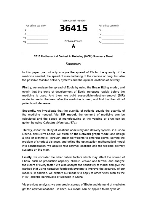
In this paper ,we not only analyze the spread of Ebola, the quantity of the medicine needed, the speed of manufacturing of the vaccine or drug, but also the possible feasible delivery systems and the optimal locations of delivery. Firstly, we analyze the spread of Ebola by using the linear fitting model, and obtain that the trend of development of Ebola increases rapidly before the medicine is used. And then, we build susceptible-infective-removal (SIR) model to predict the trend after the medicine is used, and find that the ratio of patients will decrease. Secondly, we investigate that the quantity of patients equals the quantity of the medicine needed. Via SIR model, the demand of medicine can be calculated and the speed of manufacturing of the vaccine or drug can be gotten by using Calculus (Newton.1671). Thirdly, as for the study of locations of delivery and delivery system, in Guinea, Liberia, and Sierra Leone, we establish the Network graph model and design a kind of arithmetic. Through attaching weights to different points, solving the problem of shortest distance, and taking the optimization mathematical model into consideration, we acquire four optimal locations and the feasible delivery systems on the map. Finally, we consider the other critical factors which may affect the spread of Ebola, such as production capacity, climate, vehicle and terrain, and analyze the extent of every factor. We also analyze the sensitivity of model and give the method that using negative feedback system to improve the accuracy of our models. In addition, we explore our models to apply to other fields such as the H1N1 and the earthquake of Sichuan in China. Via previous analysis, we can predict spread of Ebola and demand of medicine, get the optimal locations. Besides, our model can be applied to many fields.
美国大学生数学建模大赛英文写作

写作要求 : 1. 简短 论文标题一般在10个字内,最多不超 过15个词。
多用复合词
如:self-design, cross-sectional, dust-free, water-proof, input-orientation, piece-wiselinear 利用缩略词 如:e.g., i.e., vs.(与…相对), ibid.(出处相同), etc., cit.(在上述引文中), et al.(等人), viz.(即,就是), DEA (data envelopment analysis), OLS(Ordinary least-squares)
“Investigation on …”, “Observation on …”, “The Method of …”, “Some thought on…”, “A research on…”等冗余套语 。
4. 少用问题性标题 5. 避免名词与动名词混杂使用 如:标题是 “The Treatment of Heating and Eutechticum of Steel” 宜改为 “Heating and Eutechticuming of Steel” 6. 避免使用非标准化的缩略语 论文标题要 求简洁,但一般不使用缩略语 ,更不能使用 非标准化的缩略语 。
关键词(Keywords)
基本功能:顾名思义;便于检索 语言特点:多用名词;字数有限(4-6); 出处明确 写作要求 :论文的关键字一般列在作者与单 位之下,论文摘要之上。也有列在论文摘 要之下的。关键词除第一个字母大写外, 一般不要求大写。关键词间用逗号、分号 或大间隔隔开。最末一个关键词一般不加 用逗号、分号或句号。
美国大学生数学建赛论文模板【范文】
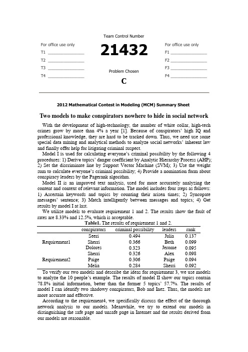
For office use onlyT1________________ T2________________ T3________________ T4________________Team Control Number21432Problem ChosenCFor office use onlyF1________________F2________________F3________________F4________________2012 Mathematical Contest in Modeling (MCM) Summary SheetTwo models to make conspirators nowhere to hide in social network With the development of high-technology, the number of white collar, high-tech crimes grow by more than 4% a year [1]. Bec ause of conspirators’ high IQ and professional knowledge, they are hard to be tracked down. Thus, we need use some special data mining and analytical methods to analyze social networks’ inherent law and finally offer help for litigating criminal suspect.M odel I is used for calculating everyone’s criminal possibility by the following 4 procedures: 1) Derive topics’ danger coefficient by Ana lytic Hierarchy Process (AHP);2) Set the discriminate line by Support Vector Machine (SVM); 3) Use the weight sum to c alculate everyone’s criminal possibility; 4) Provide a nomination form about conspiracy leaders by the Pagerank algorithm.Model II is an improved text analysis, used for more accurately analyzing the content and context of relevant information. The model includes four steps as follows: 1) Ascertain keywords and topics by counting their arisen times; 2) Syncopate me ssages’ sentence; 3) Match intelligently between messages and topics; 4) Get results by model I at last.We utilize models to evaluate requirement 1 and 2. The results show the fault of rates are 8.33% and 12.5%, which is acceptable.Table1. The results of requirement 1 and 2.conspirators criminal possibility leaders rankRequirement1Seeri 0.494 Julia 0.137 Sherri 0.366 Beth 0.099 Dolores 0.323 Jerome 0.095Requirement2 Sherri 0.326 Alex 0.098 Paige 0.306 Paige 0.094 Melia 0.284 Sherri 0.092To verify our two models and describe the ideas for requirement 3, we use models to analyze the 10 people’s example. The results of model II sho w our topics contain 78.8% initial information, better than the former 5 topics’ 57.7%. The results of model I can identify two shadowy conspirators, Bob and Inez. Thus, the models are more accurate and effective.According to the requirement4, we specifically discuss the effect of the thorough network analysis to our models. Meanwhile, we try to extend our models in distinguishing the safe page and unsafe page in Internet and the results derived from our models are reasonable.Two models to make conspirators nowhere to hideTeam #13373February 14th ,2012ContentIntroduction (3)The Description of the Problem (3)Analysis (3)What is the goal of the Modeling effort? (4)Flow chart (4)Assumptions (5)Terms, Definitions and Symbols (5)Model I (6)Overview (6)Model Built (6)Solution and Result (9)Analysis of the Result (10)Model II (11)Overview (11)Model Built (11)Result and Analysis (12)Conclusions (13)Technical summary (13)Strengths and Weaknesses (13)Extension (14)Reference (14)Appendix (16)IntroductionWith the development of our society, more and more high-tech conspiracy crimes and white-collar crimes take place in business and government professionals. Unlike simple violent crime, it is a kind of bran-new crime style, would gradually create big fraud schemes to hurt others’ benefit and destroy business companies.In order to track down the culprits and stop scams before they start, we must make full use of effective simulation model and methodology to search their criminal information. We create a Criminal Priority Model (CPM) to evaluate every suspect’s criminal possibility by analyzing text message and get a priority line which is helpful to ICM’s investigation.In addition, using semantic network analysis to search is one of the most effective ways nowadays; it will also be helpful we obtain and analysis semantic information by automatically extract networks using co-occurrence, grammatical analysis, and sentiment analysis. [1]During searching useful information and data, we develop a whole model about how to effective search and analysis data in network. In fact, not only did the coalescent of text analysis and disaggregated model make a contribution on tracking down culprits, but also provide an effective way for analyzing other subjects. For example, we can utilize our models to do the classification of pages.In fact, the conditions of pages’classification are similar to criminological analysis. First, according to the unsafe page we use the network crawler and Hyperlink to find the pages’ content and the connection between each pages. Second, extract the messages and the relationships between pages by Model II. Third, according to the available information, we can obtain the pages’priority list about security and the discriminate line separating safe pages and the unsafe pages by Model I. Finally we use the pages’ relationships to adjust the result.The Description of the ProblemAnalysisAfter reading the whole ICM problem, we make a depth analysis about the conspiracy and related information. In fact, the goal of ICM leads us to research how to take advantage of the thorough network, semantic, and text analyses of the message contents to work out personal criminal possibility.At first, we must develop a simulation model to analysis the current case’s data, and visualize the discriminate line of separating conspirator and non-conspirator.Then, by increasing text analyses to research the possible useful information from “Topic.xls”, we can optimize our model and develop an integral process of automatically extract and operate database.At last, use a new subject and database to verify our improved model.What is the goal of the Modeling effort?●Making a priority list for crime to present the most likely conspirators●Put forward some criteria to discriminate conspirator and non-conspirator, createa discriminate line.●Nominate the possible conspiracy leaders●Improve the model’s accuracy and the credit of ICM●Study the principle and steps of semantic network analysis●Describe how the semantic network analysis could empower our model.Flow chartFigure 1Assumptions●The messages have no serious error.●These messages and text can present what they truly mean.●Ignore special people, such as spy.●This information provided by ICM is reasonable and reliable.Terms, Definitions and SymbolsTable 2. Model parametersParameter MeaningThe rate of sending message to conspirators to total sending messageThe rate of receiving message to conspirators to total receiving messageThe dangerous possibility of one’s total messagesThe rate of messages with known non-conformist to total messagesDanger coefficient of topicsThe number of one’s sending messagesThe number of one’s receiving messagesThe number of one’s sending messages from criminalThe number of one’s receiving messages from criminalThe number of one’s sending messages from non-conspiratorThe number of one’s receiving messages from non-conspiratorDanger coefficient of peopleModel IOverviewModel I is used for calculating and analyzing everyone’s criminal possibility. In fact, the criminal possibility is the most important parameter to build a priority list and a discriminate line. The model I is made up of the following 4 procedures: (1) Derive topics’danger coefficient by Analytic Hierarchy Process (AHP); (2) Set the discriminate line by Support Vector Machine (SVM); (3) Use the weight sum to calculate everyone’s criminal possibility; (4) Provide a nomination form about conspiracy leaders by the Pagerank algorithm.Model BuiltStep.1PretreatmentIn order to decide the priority list and discriminate line, we must sufficiently study the data and factors in the ICM.For the first, we focus on the estimation about the phenomena of repeated names. In the name.xls, there are three pair phenomena of repeated names. Node#7 and node#37 both call Elsie, node#16 and node#34 both call Jerome, node#4 and node#32 both calls Gretchen. Thus, before develop simulation models; we must evaluate who are the real Elsie, Jerome and Gretchen.To decide which one accord with what information the problem submitsFirst we study the data in message.xls ,determine to analysis the number of messages of Elsie, Jerome and Gretchen. Table1 presents the correlation measure of their messages with criminal topic.Figure2By studying these data and figures, we can calculate the rate of messages about criminal topic to total messages; node#7 is 0.45455, while node#37 is 0.27273. Furthermore node#7 is higher than node#37 in the number of messages.Thus, we evaluate that node #7 is more likely Elsie what the ICM points out.In like manner, we think node#34, node#32 are those senior managers the ICM points out. In the following model and deduction, we assume node#7 is Elsie, node#34 is Jerome and node #32 is Gretchen.Step.2Derive topics’ danger coefficient by Analytic Hierarchy ProcessUse analytic hierarchy process to calculate the danger every topic’s coefficient. During the research, we decide use four factors’ effects to evaluate :● Aim :Evaluate the danger coefficient of every topic.[2]● Standard :The correlation with dangerous keywordsThe importance of the topic itselfThe relationship of the topic and known conspiratorsThe relationship of the topic and known non-conspirators● Scheme : The topics (1,2,3……15)Figure3According to previous research, we decide the weight of The Standard to Aim :These weights can be evaluated by paired comparison algorithm, and build a matrix about each part.For example, build a matrix about Standard and Aim, the equation is followingij j i a C C ⇒:ijji ij n n ij a a a a A 1,0)(=>=⨯ The other matrix can be evaluated by the similar ways. At last, we make a consistency check to matrix A and find it is reasonable.The result shows in the table, and we can use the data to continue the next model. Step.3 Use the weight sum to calculate everyone ’s criminal possibilityWe will start to study every one’s danger coefficient by using four factors,, and .[3]100-第一份工作开始时间)(第一份工作结束时间第一份工作持续时间=The first factor means calculate the rate of someone’s sending criminal messages to total sending messages.The second factors means calculate the rate of someone’s receivingcriminal messages to total receiving messages.=The third factormeans calculate the dangerous possibility of someone’stotal messages.The four factorthe rate of someone’s messages with non-conspirators tototal messages.At last, we use an equation to calculate every one’s criticality, namely thepossibility of someone attending crime. ( Shows every factors’weighing parameter)After calculating these equations abov e, we derive everyone’s criminal possibilityand a priority list. (See appendix for complete table about who are the most likely conspirators) We instead use a cratering technique first described by Rossmo [1999]. The two-dimensional crime points xi are mapped to their radius from the anchor point ai, that is, we have f : xi → ri, where f(xi) = j i i a a (a shifted modulus). The set ri isthen used to generate a crater around the anchor point.There are two dominatingStep.4 Provide a nomination form about conspiracy leaders by the Pagerankalgorithm.At last, we will find out the possible important leaders by pagerank model, and combined with priority list to build a prior conspiracy leaders list.[4]The essential idea from Page Rank is that if node u has a link to node v, then the author of u is an implicitly conferring some importance to node v. Meanwhile it means node v has a important chance. Thus, using B (u) to show the aggregation of links to node u, and using F (u) to show the aggregation of received links of node u, The C is Normalization factor. In each iteration, propagate the ranks as follows: The next equation shows page rank of node u:Using the results of Page Rank and priority list, we can know those possiblecriminal conspiracy leaders.Solution and ResultRequirement 1:According to Model I above, we calculate these data offered by requirement 1 and build two lists. The following shows the result of requirement 1.By running model I step2, we derive danger coefficient of topics, the known conspiracy topic 7, 11 and 13 are high danger coefficient (see appendix Table4. for complete information).After running model step3, we get a list of every one’s criticality .By comparing these criticality, we can build a priority list about criminal suspects. In fact, we find out criminal suspects are comparatively centralized, who are highly different from those known non-conspirators. This illuminates our model is relative reasonable. Thus we decide use SVM to get the discriminate line, namely to separate criminal suspects and possible non-conspirators (see appendix Table5. for complete information). Finally, we utilize Page rank to calculate criminal suspects’ Rank and status, table4 shows the result. Thus, we nominate 5 most likely criminal leaders according the results of table4.They are Julia, Beth, Jerome, Stephanie and Neal.According to the requirement of problem1, we underscore the situations of three senior managers Jerome, Delores and Gretchen. Because the SVM model makes a depth analysis about conspirators, Jerome is chosen as important conspirator, Delores and Gretchen both has high danger coefficient. We think Jerome could be a conspirator, while Delores and Gretchen are regarded as important criminal suspects. Using the software Ucinet, we derive a social network of criminal suspects.The blue nodes represent non-conspirators. The red nodes represent conspirators. The yellow nodes represent conspiracy leaders.Figure 4Requirement 2:Using the similar model above, we can continue analyzing the results though theconditions change.We derive three new tables (4, 5 and 6): danger coefficient of topics, every one’s criticality and the probability of nominated. At last, we get a new priority list (table6) and 5 most likely criminal leaders: Alex, Sherri, Yao, Elsie and Jerome.We sincerely wish that our analysis can be helpful to ICM’s investigation. We figure out a new figure, which shows the social network of criminal suspects for requirement 2.Figure 5Analysis of the Result1)AnalysisIn the requirement 1, we find out 24 possible criminal suspects. All of 7 known conspirators are in the 24 suspects and their danger coefficients are also pretty high. However, there are 2 known non-conspirators are in these suspects.Thus, the rate of making mistakes is 8.33%. In all, we still have enough reasons to think the model is reasonable.In addition, we find 5 suspects who are likely conspirators by Support Vector Machine (SVM).In the requirement 2, we also choose 24 the most likely conspirators after run our CPM. All of 8 known conspirators are also in the 24 suspects and their danger coefficients are pretty high. Because 3 known non-conspirators are in these suspects, the rate of making mistakes is 12.5%, which is higher to the result of requirement 1.2)ComparisonTo research the effect of changing the number of criminal topics and conspirators to results, we decide to do an additional research about their effect.We separate the change of topics and crimes’numbers, analysis result’s changes of only one factor:In order to analyze the change between requirement 1 and 2, we choose those people whose rank has a big change over 30.Reference: the node.1st result: the part of the requirement1’s priority list.2nd result: the part of the requirement2’s priority list.3rd result: the priority’s changes of requirement 1 and 2.After investigate these people, we find out the topics about them isn’t close connected with node#0. Thus, the change of node#0 does not make a great effect on their change.However, there are more than a half of people who talk about topic1. According to the analysis, we find the topic1 has a great effect on their change. The topic1 is more important to node#0.Thus; we can do an assumption that the decision of topics has bigger effect on the decision of the personal identity and decide to do a research in the following content.Model IIOverviewAccording to requirement3, we will take the text analysis into account to enhance our model. In the paper, text analysis is presented as a paradigm for syntactic-semantic analysis of natural language. The main characteristics of this approach are: the vectors of messages about keywords, semanteme and question formation. In like manner, we need get three vectors of topics. Then, we utilize similarity to separate every message to corresponding topics. Finally, we evaluate these effects of text analysis by model I.Model BuiltStep.1PretreatmentIn this step, we need conclude relatively accurate topics by keywords in messages. Not only builds a database about topics, but also builds a small database for adjusting the topic classification of messages. The small database for adjusting is used for studying possible interpersonal relation between criminal suspects, i. e. Bob always use positive and supportive words to comment topics and things about Jerry, and then we think Bob’s messages are closely connected with topics about Jerry. [5] At first, we need to count up how many keywords in the whole messages.Text analysis is word-oriented, i.e., the word plays the central role in language understanding. So we avoid stipulating a grammar in the traditional sense and focus on the concept of word. During the analysis of all words in messages, we ignore punctuation, some simple word such as “is” and “the”, and extract relative importantwords.Then, a statistics will be completed about how many times every important word occurs. We will make a priority list and choose the top part of these words.Finally, according to some messages, we will turn these keywords into relatively complete topics.Step.2Syncopate sentenceWe will make a depth research to every sentence in messages by running program In the beginning, we can utilize the same way in step1 to syncopate sentence, deriving every message’s keywords. We decide create a vector about keywords: = () (m is the number keywords in everymessage)For improving the accuracy and relativity of our keywords, we decide to build a vector that shows every keyword’s synonyms, antonym.= () (1<k<m, p is the number of correlative words)According to primary analysis, we can find some important interpersonal relations between criminal suspects, i.e. Bob is closely connected with Jerry, then we can build a vector about interpersonal relation.= () (n is the number of relationships in one sentence )Step.3Intelligent matchingIn order to improve the accuracy of our disaggregated model, we use three vectors to do intelligent matching.Every message has three vectors:. Similarly, every topic alsohas three vectors.At last, we can do an intelligent matching to classify. [6]Step.4Using CPMAfter deriving new the classification of messages, we will make full use of new topics to calculate every one’s criticality.Result and AnalysisAfter calculating the 10 people example, we derive new topics. By verifying the topics’ contained initial information, we can evaluate the effect of models.The results of model II show our topics contain 78.8% initial information, better than former 5 topics’ 57.7%.T hus, new topics contain more initial information. Meanwhile, we build a database about interpersonal relation, and using it to optimize the results of everyone’s criminal possibility.Table 3#node primary new #node primary new1 0 0.065 6 0.342 0.2652 0.342 0.693 7 0.891 0.9123 0.713 0.562 8 0.423 0.354 1 1 9 0.334 0.7235 0.823 0.853 10 0.125 0.15 The results of model I can identify the two shadowy conspirators, Bob and Inez. In the table, the rate of fault is becoming smaller.According to Table11, we can derive some information:1.Analysis the danger coefficient of two people, Bob and Inez. Bob is theperson who self-admitted his involvement in a plan bargain for a reducedsentence. His data changes from 0.342 to 0.693. And Inez is the person whogot off, his data changes from 0.334 to 0.723. The models can identify thetwo shadowy people.2.Carol, the person who was later dropped his data changes from 0.713 to0.562. Although it still has a relatively high danger coefficient, the resultsare enhancing by our models.3.The distance between high degree people and low degree become bigger, itpresents the models would more distinctly identify conspirators andnon-conspirators.Thus, the models are more accurate and effective.ConclusionsTechnical summaryWe bring out a whole model about how to extract and analysis plentiful network information, and finally solve the classification problems. Four steps are used to make the classification problem easier.1)According known conspirators and correlative information, use resemblingnetwork crawler to extract what we may need information and messages.[7]2)Using the second model to analysis and classify these messages and text, getimportant topics.3)Using the first model to calculate everyone’s criminal possibility.4)Using an interpersonal relation database derived by step2 to optimize theresults. [8]Strengths and WeaknessesStrengths:1)We analyze the danger coefficient of topics and people by using different characteristics to describe them. Its results have a margin of error of 10percentage points. That the Models work well.2)In the semantic analysis, in addition to obtain topics from messages in social network, we also extract the relationships of people and adjust the final resultimprove the model.3)We use 4 characteristics to describe people’s danger coefficient. SVM has a great advantage in classification by small characteristics. Using SVM to classify the unknown people and its result is good.Weakness:1)For the special people, such as spy and criminal researcher, the model works not so well.2)We can determine some criminals by topics; at the same time we can also use the new criminals to adjust the topics. The two react upon each other. We canexpect to cycle through several times until the topics and criminals are stable.However we only finish the first cycle.3)For the semantic analysis model we have established, we just test and verify in the example (social network of 10 people). In the condition of large social network, the computational complexity will become greater, so the classify result is still further to be surveyed.ExtensionAccording to our analysis, not only can our model be applied to analyze criminal gangs, but also applied to similar network models, such as cells in a biological network, safe pages in Internet and so on. For the pages’ classification in Internet, our model would make a contribution. In the following, we will talk about how to utilize [9] Our model in pages’ classification.First, according to the unsafe page we use the network crawler and Hyperlink to find the pages’content and the connection between each page. Second, extract the messages and the relationships between pages by Model II. Third, according to the available information, we can obtain the pages’priority list about security and the discriminate line separating safe pages and the unsafe pages by Model I. Finally we use the pages’ relationships to adjust the result.Reference1. http://books.google.pl/books?id=CURaAAAAYAAJ&hl=zh-CN2012.2. AHP./wiki/%E5%B1%82%E6%AC%A1%E5%88%86%E6%9E%90%E6%B 3%95.3. Schaller, J. and J.M.S. Valente, Minimizing the weighted sum of squared tardiness on a singlemachine. Computers & Operations Research, 2012. 39(5): p. 919-928.4. Frahm, K.M., B. Georgeot, and D.L. Shepelyansky, Universal emergence of PageRank.Journal of Physics a-Mathematical and Theoretical, 2011. 44(46).5. Park, S.-B., J.-G. Jung, and D. Lee, Semantic Social Network Analysis for HierarchicalStructured Multimedia Browsing. Information-an International Interdisciplinary Journal, 2011.14(11): p. 3843-3856.6. Yi, J., S. Tang, and H. Li, Data Recovery Based on Intelligent Pattern Matching.ChinaCommunications, 2010. 7(6): p. 107-111.7. Nath, R. and S. Bal, A Novel Mobile Crawler System Based on Filtering off Non-ModifiedPages for Reducing Load on the Network.International Arab Journal of Information Technology, 2011. 8(3): p. 272-279.8. Xiong, F., Y. Liu, and Y. Li, Research on Focused Crawler Based upon Network Topology.Journal of Internet Technology, 2008. 9(5): p. 377-380.9. Huang, D., et al., MyBioNet: interactively visualize, edit and merge biological networks on theWeb. Bioinformatics, 2011. 27(23): p. 3321-3322.AppendixTable 4requirement 1topic danger topic danger topic danger topic danger7 1.65 4 0.78 5 0.47 8 0.1713 1.61 10 0.77 15 0.46 14 0.1711 1.60 12 0.47 9 0.19 6 0.141 0.812 0.473 0.18requirement 2topic danger topic danger topic danger topic danger1 0.402 0.26 15 0.15 14 0.117 0.37 9 0.23 8 0.15 3 0.0913 0.37 10 0.21 5 0.14 6 0.0611 0.30 12 0.18 4 0.12Table 5requirement 1#node danger #node danger #node danger #node danger 21 0.74 22 0.19 0 0.13 23 0.03 67 0.69 4 0.19 40 0.13 72 0.03 54 0.61 33 0.19 36 0.13 62 0.03 81 0.49 47 0.19 11 0.12 51 0.02 7 0.47 41 0.19 69 0.12 57 0.02 3 0.37 28 0.18 29 0.12 64 0.02 49 0.36 16 0.18 12 0.11 71 0.02 43 0.36 31 0.17 25 0.11 74 0.01 10 0.32 37 0.17 82 0.11 58 0.01 18 0.29 27 0.16 60 0.10 59 0.01 34 0.29 45 0.16 42 0.10 70 0.00 48 0.28 50 0.16 65 0.09 53 0.00 20 0.27 24 0.16 9 0.09 76 0.00 15 0.27 44 0.16 5 0.09 61 0.00 17 0.26 38 0.16 66 0.09 75 -0.01 2 0.23 13 0.16 26 0.08 77 -0.01 32 0.23 35 0.15 39 0.06 55 -0.02 30 0.20 1 0.15 80 0.04 68 -0.02 73 0.20 46 0.15 78 0.04 52 -0.0319 0.20 8 0.14 56 0.03 63 -0.03 14 0.19 6 0.14 79 0.03requirement 2#node danger #node danger #node danger #node danger 0 0.39881137 75 0.1757106 47 0.1090439 11 0.0692506 21 0.447777778 52 0.1749354 71 0.1089147 4 0.0682171 67 0.399047158 38 0.1738223 82 0.1088594 42 0.0483204 54 0.353754153 10 0.1656977 14 0.1079734 65 0.046124 81 0.325736434 19 0.1559173 27 0.1060724 60 0.0459948 2 0.306054289 40 0.1547065 23 0.105814 39 0.0286822 18 0.303178295 30 0.1517626 5 0.1039406 62 0.0245478 66 0.28372093 80 0.145155 8 0.10228 78 0.0162791 7 0.279870801 24 0.1447674 73 0.1 56 0.0160207 63 0.261886305 70 0.1425711 50 0.0981395 64 0.0118863 68 0.248514212 29 0.1425562 26 0.097213 72 0.011369548 0.239668277 45 0.1374667 1 0.0952381 79 0.009302349 0.238076781 37 0.1367959 69 0.0917313 51 0.0056848 34 0.232614868 17 0.1303064 33 0.0906977 57 0.0056848 3 0.225507567 6 0.1236221 31 0.0905131 74 0.0054264 35 0.222435188 22 0.1226934 36 0.0875452 76 0.005168 77 0.214470284 13 0.1222868 41 0.0822997 53 0.0028424 20 0.213718162 44 0.115007 46 0.0749354 58 0.0015504 43 0.204328165 12 0.1121447 28 0.0748708 59 0.0015504 32 0.193311469 15 0.1121447 16 0.074234 61 0.0007752 55 0.182687339 9 0.1117571 25 0.0701292Table 6requirement 1#node leader #node leader #node leader #node leader 15 0.1368 49 0.0481 7 0.0373 19 0.0089 14 0.0988 4 0.0423 21 0.0357 32 0.0073 34 0.0951 10 0.0422 18 0.029 22 0.0059 30 0.0828 67 0.0421 48 0.0236 81 0.0053 17 0.0824 54 0.0377 20 0.0232 73 043 0.0596 3 0.0377 2 0.0181 33 0requirement 2#node leader #node leader #node leader #node leader 21 0.0981309 7 0.0714406 54 0.0526831 43 0.01401872 0.0942899 34 0.0707246 32 0.0464614 81 0.00977763 0.0916127 0 0.0706746 18 0.041114248 0.0855984 20 0.0658119 68 0.028532867 0.0782211 49 0.0561665 35 0.024741。
MCM北美数学建模论文模版

Title Abstract:Key words:Contents1. Introduction............................................................................ .. (3)1.1 Why does toll way collects toll? (3)1.2 Toll modes (3)1.3 Toll collection methods (3)1.4 Annoyance in toll plazas (3)1.5 The origin of the toll way problem (3)1.6 Queuing theory (4)2. The Description of Problem................................................................................... .. (5)2.1 How do we approximate the whole course of payingtoll? (5)2.2 How do we define the optimalconfiguration? (5)2.2.1 From the perspective of motorist (5)2.2.2 From the perspective of the toll plaza (6)2.2.3 Compromise (6)2.3 Overall optimization and local optimization (6)2.4 The differences in weights and sizes of vehicles (7)2.5 What if there is no dataavailable? ............................................................................. .. (7)3. Models......................................................................................... .. (7)3.1 Basic Model.................................................................................. .. (7)3.1.1 Symbols andDefinitions (7)3.1.2 Assumptions (8)3.1.3 The Foundation of Model (9)3.1.4 Solution and Result (11)3.1.5 Analysis of the Result (11)3.1.6 Strength and Weakness (13)3.2 Improved Model.............................................................. .. (14)3.2.1 Extra Symbols (14)3.2.2 Additional Assumptions (14)3.2.3 The Foundation of Model (14)3.2.4 Solution and Result (15)3.2.5 Analysis of the Result (18)3.2.6 Strength and Weakness (19)4. Conclusions............................................................................. (19)4.1 Conclusions of the problem (19)4.2 Methods used in our models (19)4.3 Application of our models (19)5. Future Work...................................................................................... .. (19)5.1 Another model………………………………………………………………………………………195.2 Another layout of toll plaza (23)5.3 The newly- adopted charging methods (23)6. References.............................................................................. (23)7. Appendix................................................................................. (23)Programs and codes………………………………………………………………..……………………24I. IntroductionIn order to indicate the origin of the toll way problems, the following background is worth mentioning.1.11.21.31.41.51.6II. The Description of the Problem2.1 How do we approximate the whole course of paying toll?●●●●2.2 How do we define the optimal configuration?1) From the perspective of motorist:2) From the perspective of the toll plaza:3) Compromise:2.3 The local optimization and the overall optimization●●●Virtually:2.4 The differences in weights and sizes of vehicles2.5 What if there is no data available?III. Models3.1 Basic Model3.1.1 Terms, Definitions and SymbolsThe signs and definitions are mostly generated from queuing theory.●●●●●3.1.2 Assumptions●●●●●3.1.3 The Foundation of Model1) The utility function●The cost of toll plaza:●The loss of motorist:●The weight of each aspect:●Compromise:2) The integer programmingAccording to queuing theory, we can calculate the statistical properties as follows.3)The overall optimization and the local optimization●The overall optimization:●The local optimization:●The optimal number of tollbooths:3.1.4 Solution and Result1) The solution of the integer programming:2) Results:3.1.5 Analysis of the Result●Local optimization and overall optimization:●Sensitivity: The result is quite sensitive to the change of thethree parameters●Trend:●Comparison:3.1.6 Strength and Weakness●Strength: In despite of this, the model has proved that .Moreover, we have drawn some useful conclusions about . T hemodel is fit for, such as●Weakness: This model just applies to . As we have stated, .That’s just what we should do in the improved model.3.2 Improved Model3.2.1 Extra SymbolsSigns and definitions indicated above are still valid. Here are some extra signs and definitions.●●●●3.2.2 Additional Assumptions●●●Assumptions concerning the anterior process are the same as the Basic Model.3.2.3 The Foundation of Model1) How do we determine the optimal number?As we have concluded from the Basic Model,3.2.4 Solution and Result1) Simulation algorithmBased on the analysis above, we design our simulation arithmetic as follows.●Step1:●Step2:●Step3:●Step4:●Step5:●Step6:●Step7:●Step8:●Step9:2) Flow chartThe figure below is the flow chart of the simulation.3) Solution3.2.5 Analysis of the Result3.2.6 Strength and Weakness●Strength: The Improved Model aims to make up for the neglectof . The result seems to declare that this model is more reasonable than the Basic Model and much more effective than the existing design.●Weakness: . Thus the model is still an approximate on a largescale. This has doomed to limit the applications of it.IV. Conclusions4.1 Conclusions of the problem●●●4.2 Methods used in our models●●●4.3 Applications of our models●●●V. Future Work 5.1 Another model5.1.1The limitations of queuing theory 5.1.25.1.35.1.41)●●●●2)●●●3)●●●4)标准实用5.2 Another layout of toll plaza5.3 The newly- adopted charging methodsVI. References[1][2][3][4][5]VII. Appendix文案大全。
美赛-数学建模 模版
摘要第一段:写论文解决什么问题1.问题的重述其中主要的内容是a. 介绍重点词开头:例1:“Hand move” irrigation, a cheap but labor-intensive system used on small farms, consists of a movable pipe with sprinkler on top that can be attached to a stationary main.例2:……is a real-life common phenomenon with many complexities.例3:An (effective plan) is crucial to………b. 直接指出问题:例1:We find the optimal number of tollbooths in a highway toll-plaza for a given number of highway lanes: the number of tollbooths that minimizes average delay experienced by cars.例2:A brand-new university needs to balance the cost of information technology security measures with the potential cost of attacks on its systems.例3:We determine the number of sprinklers to use by analyzing the energy and motion of water in the pipe and examining the engineering parameters of sprinklers available in the market.例4: After mathematically analyzing the ……problem, our modeling group would like to present our conclusions, strategies, (and recommendations )to the …….例5:Our goal is... that (minimizes the time )……….2.解决这个问题的伟大意义反面说明。