Adaptive Fuzzy Cognitive Maps for Hyperknowledge Representation in Strategy Formation Proce

合集下载

基于绿地八类感知属性的城市公园场所依恋影响机制

ｄｅｐｅｎｄｅｎｃｅꎬ ｗｈｉｌｅｔｈｅｃｕｌｔｕｒｅｐｅｒｃｅｐｔｉｏｎｈａｓｔｈｅｇｒｅａｔｅｓｔｉｍｐａｃｔꎬ ｆｏｌｌｏｗｅｄｂｙｓｏｃｉａｌｐｅｒｃｅｐｔｉｏｎꎻ
２) Ｃｕｌｔｕｒｅａｎｄｓｅｒｅｎｅｐｅｒｃｅｐｔｉｏｎｓｃａｎｈａｖｅａｄｉｒｅｃｔｐｏｓｉｔｉｖｅｉｍｐａｃｔｏｎｐｌａｃｅｉｄｅｎｔｉｔｙꎻ ３) Ｃｕｌｔｕｒｅꎬ ｓｏｃｉａｌꎬ
ＬｕＹｉｗｅｉＬｉｕＺｈｉｃｈｅｎｇ
( ＣｏｌｌｅｇｅｏｆＬａｎｄｓｃａｐｅＡｒｃｈｉｔｅｃｔｕｒｅꎬ ＢｅｉｊｉｎｇＦｏｒｅｓｔｒｙＵｎｉｖｅｒｓｉｔｙꎬ Ｂｅｉｊｉｎｇ１０００８３ꎬ Ｃｈｉｎａ)
Ａｂｓｔｒａｃｔ: ＡｓＣｈｉｎａｐｕｔｓｇｒｅａｔｅｒｅｍｐｈａｓｉｓｏｎｉｍｐｒｏｖｉｎｇｔｈｅｑｕａｌｉｔｙｏｆｕｒｂａｎｓｐａｃｅｓｔｏｃｋꎬ ｃｒｅａｔｉｎｇｐｌａｃｅ
ＤＯＩ: １０.１２１６９ / ｚｇｃｓｌｙ.２０２３.１０.２９.０００１
ＩｎｆｌｕｅｎｃｉｎｇＭｅｃｈａｎｉｓｍｏｆＰｌａｃｅＡｔｔａｃｈｍｅｎｔｔｏＵｒｂａｎＰａｒｋＢａｓｅｄｏｎ
ＥｉｇｈｔＰｅｒｃｅｉｖｅｄＳｅｎｓｏｒｙＤｉｍｅｎｓｉｏｎｓｉｎＧｒｅｅｎＳｐａｃｅｓ
姆斯和约瑟夫罗根巴克 [１４] 于１９８９年提出ꎬ 其
上ꎬ 瑞典学者Ｇｒａｈｎ和Ｓｔｉｇｓｄｏｔｔｅｒ通过实地调查研
种情感联结关系 [１０] ꎮ 该理论最早由丹尼尔威廉
( ＰｅｒｃｅｉｖｅｄＳｅｎｓｏｒｙＤｉｍｅｎｓｉｏｎｓꎬ ＰＳＤｓ) : １) 自然
经典二维结构包括场所认同和场所依赖两个维度ꎮ
等社会维度的因

车辆控制系统说明书

IndexAactuation layer, 132average brightness,102-103adaptive control, 43Badaptive cruise control, 129backpropagation algorithm, 159adaptive FLC, 43backward driving mode,163,166,168-169adaptive neural networks,237adaptive predictive model, 283Baddeley-Molchanov average, 124aerial vehicles, 240 Baddeley-Molchanov fuzzy set average, 120-121, 123aerodynamic forces,209aerodynamics analysis, 208, 220Baddeley-Molchanov mean,118,119-121alternating filter, 117altitude control, 240balance position, 98amplitude distribution, 177bang-bang controller,198analytical control surface, 179, 185BCFPI, 61-63angular velocity, 92,208bell-shaped waveform,25ARMAX model, 283beta distributions,122artificial neural networks,115Bezier curve, 56, 59, 63-64association, 251Bezier Curve Fuzzy PI controller,61attitude angle,208, 217Bezier function, 54aumann mean,118-120bilinear interpolation, 90, 300,302automated manual transmission,145,157binary classifier,253Bo105 helicopter, 208automatic formation flight control,240body frame,238boiler following mode,280,283automatic thresholding,117border pixels, 101automatic transmissions,145boundary layer, 192-193,195-198autonomous robots,130boundary of a fuzzy set,26autonomous underwater vehicle, 191braking resistance, 265AUTOPIA, 130bumpy control surface, 55autopilot signal, 228Index 326CCAE package software, 315, 318 calibration accuracy, 83, 299-300, 309, 310, 312CARIMA models, 290case-based reasoning, 253center of gravity method, 29-30, 32-33centroid defuzzification, 7 centroid defuzzification, 56 centroid Method, 106 characteristic polygon, 57 characterization, 43, 251, 293 chattering, 6, 84, 191-192, 195, 196, 198chromosomes, 59circuit breaker, 270classical control, 1classical set, 19-23, 25-26, 36, 254 classification, 106, 108, 111, 179, 185, 251-253classification model, 253close formation flight, 237close path tracking, 223-224 clustering, 104, 106, 108, 251-253, 255, 289clustering algorithm, 252 clustering function, 104clutch stroke, 147coarse fuzzy logic controller, 94 collective pitch angle, 209 collision avoidance, 166, 168 collision avoidance system, 160, 167, 169-170, 172collision avoidance system, 168 complement, 20, 23, 45 compressor contamination, 289 conditional independence graph, 259 confidence thresholds, 251 confidence-rated rules, 251coning angle, 210constant gain, 207constant pressure mode, 280 contrast intensification, 104 contrast intensificator operator, 104 control derivatives, 211control gain, 35, 72, 93, 96, 244 control gain factor, 93control gains, 53, 226control rules, 18, 27, 28, 35, 53, 64, 65, 90-91, 93, 207, 228, 230, 262, 302, 304-305, 315, 317control surfaces, 53-55, 64, 69, 73, 77, 193controller actuator faulty, 289 control-weighting matrix, 207 convex sets, 119-120Coordinate Measurement Machine, 301coordinate measuring machine, 96 core of a fuzzy set, 26corner cube retroreflector, 85 correlation-minimum, 243-244cost function, 74-75, 213, 282-283, 287coverage function, 118crisp input, 18, 51, 182crisp output, 7, 34, 41-42, 51, 184, 300, 305-306crisp sets, 19, 21, 23crisp variable, 18-19, 29critical clearing time, 270 crossover, 59crossover probability, 59-60cruise control, 129-130,132-135, 137-139cubic cell, 299, 301-302, 309cubic spline, 48cubic spline interpolation, 300 current time gap, 136custom membership function, 294 customer behav or, 249iDdamping factor, 211data cleaning, 250data integration, 250data mining, 249, 250, 251-255, 259-260data selection, 250data transformation, 250d-dimensional Euclidean space, 117, 124decision logic, 321 decomposition, 173, 259Index327defuzzification function, 102, 105, 107-108, 111 defuzzifications, 17-18, 29, 34 defuzzifier, 181, 242density function, 122 dependency analysis, 258 dependency structure, 259 dependent loop level, 279depth control, 202-203depth controller, 202detection point, 169deviation, 79, 85, 185-188, 224, 251, 253, 262, 265, 268, 276, 288 dilation, 117discriminated rules, 251 discrimination, 251, 252distance function, 119-121 distance sensor, 167, 171 distribution function, 259domain knowledge, 254-255 domain-specific attributes, 251 Doppler frequency shift, 87 downhill simplex algorithm, 77, 79 downwash, 209drag reduction, 244driver’s intention estimator, 148 dutch roll, 212dynamic braking, 261-262 dynamic fuzzy system, 286, 304 dynamic tracking trajectory, 98Eedge composition, 108edge detection, 108 eigenvalues, 6-7, 212electrical coupling effect, 85, 88 electrical coupling effects, 87 equilibrium point, 207, 216 equivalent control, 194erosion, 117error rates, 96estimation, 34, 53, 119, 251, 283, 295, 302Euler angles, 208evaluation function, 258 evolution, 45, 133, 208, 251 execution layer, 262-266, 277 expert knowledge, 160, 191, 262 expert segmentation, 121-122 extended sup-star composition, 182 Ffault accommodation, 284fault clearing states, 271, 274fault detection, 288-289, 295fault diagnosis, 284fault durations, 271, 274fault isolation, 284, 288fault point, 270-271, 273-274fault tolerant control, 288fault trajectories, 271feature extraction, 256fiber glass hull, 193fin forces, 210final segmentation, 117final threshold, 116fine fuzzy controller, 90finer lookup table, 34finite element method, 318finite impulse responses, 288firing weights, 229fitness function, 59-60, 257flap angles, 209flight aerodynamic model, 247 flight envelope, 207, 214, 217flight path angle, 210flight trajectory, 208, 223footprint of uncertainty, 176, 179 formation geometry, 238, 247 formation trajectory, 246forward driving mode, 163, 167, 169 forward flight control, 217 forward flight speed, 217forward neural network, 288 forward velocity, 208, 214, 217, 219-220forward velocity tracking, 208 fossil power plants, 284-285, 296 four-dimensional synoptic data, 191 four-generator test system, 269 Fourier filter, 133four-quadrant detector, 79, 87, 92, 96foveal avascular zone, 123fundus images, 115, 121, 124 fuselage, 208-210Index 328fuselage axes, 208-209fuselage incidence, 210fuzz-C, 45fuzzifications, 18, 25fuzzifier, 181-182fuzzy ACC controller, 138fuzzy aggregation operator, 293 fuzzy ASICs, 37-38, 50fuzzy binarization algorithm, 110 fuzzy CC controller, 138fuzzy clustering algorithm, 106, 108 fuzzy constraints, 286, 291-292 fuzzy control surface, 54fuzzy damage-mitigating control, 284fuzzy decomposition, 108fuzzy domain, 102, 106fuzzy edge detection, 111fuzzy error interpolation, 300, 302, 305-306, 309, 313fuzzy filter, 104fuzzy gain scheduler, 217-218 fuzzy gain-scheduler, 207-208, 220 fuzzy geometry, 110-111fuzzy I controller, 76fuzzy image processing, 102, 106, 111, 124fuzzy implication rules, 27-28 fuzzy inference system, 17, 25, 27, 35-36, 207-208, 302, 304-306 fuzzy interpolation, 300, 302, 305- 307, 309, 313fuzzy interpolation method, 309 fuzzy interpolation technique, 300, 309, 313fuzzy interval control, 177fuzzy mapping rules, 27fuzzy model following control system, 84fuzzy modeling methods, 255 fuzzy navigation algorithm, 244 fuzzy operators, 104-105, 111 fuzzy P controller, 71, 73fuzzy PD controller, 69fuzzy perimeter, 110-111fuzzy PI controllers, 61fuzzy PID controllers, 53, 64-65, 80 fuzzy production rules, 315fuzzy reference governor, 285 Fuzzy Robust Controller, 7fuzzy set averages, 116, 124-125 fuzzy sets, 7, 19, 22, 24, 27, 36, 45, 115, 120-121, 124-125, 151, 176-182, 184-188, 192, 228, 262, 265-266fuzzy sliding mode controller, 192, 196-197fuzzy sliding surface, 192fuzzy subsets, 152, 200fuzzy variable boundary layer, 192 fuzzyTECH, 45Ggain margins, 207gain scheduling, 193, 207, 208, 211, 217, 220gas turbines, 279Gaussian membership function, 7 Gaussian waveform, 25 Gaussian-Bell waveforms, 304 gear position decision, 145, 147 gear-operating lever, 147general window function, 105 general-purpose microprocessors, 37-38, 44genetic algorithm, 54, 59, 192, 208, 257-258genetic operators, 59-60genetic-inclined search, 257 geometric modeling, 56gimbal motor, 90, 96global gain-scheduling, 220global linear ARX model, 284 global navigation satellite systems, 141global position system, 224goal seeking behaviour, 186-187 governor valves80, 2HHamiltonian function, 261, 277 hard constraints, 283, 293 heading angle, 226, 228, 230, 239, 240-244, 246heading angle control, 240Index329heading controller, 194, 201-202 heading error rate, 194, 201 heading speed, 226heading velocity control, 240 heat recovery steam generator, 279 hedges, 103-104height method, 29helicopter, 207-212, 214, 217, 220 helicopter control matrix, 211 helicopter flight control, 207 Heneghan method, 116-117, 121-124heuristic search, 258 hierarchical approaches, 261 hierarchical architecture, 185 hierarchical fuzzy processors, 261 high dimensional systems, 191 high stepping rates, 84hit-miss topology, 119home position, 96horizontal tail plane, 209 horizontal tracker, 90hostile, 223human domain experts, 255 human visual system, 101hybrid system framework, 295 hyperbolic tangent function, 195 hyperplane, 192-193, 196 hysteresis thres olding, 116-117hIIF-THEN rule, 27-28image binarization, 106image complexity, 104image fuzzification function, 111 image segmentation, 124image-expert, 122-123indicator function, 121inert, 223inertia frame, 238inference decision methods, 317 inferential conclusion, 317 inferential decision, 317 injection molding process, 315 inner loop controller, 87integral time absolute error, 54 inter-class similarity, 252 internal dependencies, 169 interpolation property, 203 interpolative nature, 262 intersection, 20, 23-24, 31, 180 interval sets, 178interval type-2 FLC, 181interval type-2 fuzzy sets, 177, 180-181, 184inter-vehicle gap, 135intra-class similarity, 252inverse dynamics control, 228, 230 inverse dynamics method, 227 inverse kinema c, 299tiJ - Kjoin, 180Kalman gain, 213kinematic model, 299kinematic modeling, 299-300 knowledge based gear position decision, 148, 153knowledge reasoning layer, 132 knowledge representation, 250 knowledge-bas d GPD model, 146eLlabyrinths, 169laser interferometer transducer, 83 laser tracker, 301laser tracking system, 53, 63, 65, 75, 78-79, 83-85, 87, 98, 301lateral control, 131, 138lateral cyclic pitch angle, 209 lateral flapping angle, 210 leader, 238-239linear control surface, 55linear fuzzy PI, 61linear hover model, 213linear interpolation, 300-301, 306-307, 309, 313linear interpolation method, 309 linear optimal controller, 207, 217 linear P controller, 73linear state feedback controller, 7 linear structures, 117linear switching line, 198linear time-series models, 283 linguistic variables, 18, 25, 27, 90, 102, 175, 208, 258Index 330load shedding, 261load-following capabilities, 288, 297 loading dock, 159-161, 170, 172 longitudinal control, 130-132 longitudinal cyclic pitch angle, 209 longitudinal flapping angle, 210 lookup table, 18, 31-35, 40, 44, 46, 47-48, 51, 65, 70, 74, 93, 300, 302, 304-305lower membership functions, 179-180LQ feedback gains, 208LQ linear controller, 208LQ optimal controller, 208LQ regulator, 208L-R fuzzy numbers, 121 Luenburger observer, 6Lyapunov func on, 5, 192, 284tiMMamdani model, 40, 46 Mamdani’s method, 242 Mamdani-type controller, 208 maneuverability, 164, 207, 209, 288 manual transmissions, 145 mapping function, 102, 104 marginal distribution functions, 259 market-basket analysis, 251-252 massive databases, 249matched filtering, 115 mathematical morphology, 117, 127 mating pool, 59-60max member principle, 106max-dot method, 40-41, 46mean distance function, 119mean max membership, 106mean of maximum method, 29 mean set, 118-121measuring beam, 86mechanical coupling effects, 87 mechanical layer, 132median filter, 105meet, 7, 50, 139, 180, 183, 302 membership degree, 39, 257 membership functions, 18, 25, 81 membership mapping processes, 56 miniature acrobatic helicopter, 208 minor steady state errors, 217 mixed-fuzzy controller, 92mobile robot control, 130, 175, 181 mobile robots, 171, 175-176, 183, 187-189model predictive control, 280, 287 model-based control, 224 modeless compensation, 300 modeless robot calibration, 299-301, 312-313modern combined-cycle power plant, 279modular structure, 172mold-design optimization, 323 mold-design process, 323molded part, 318-321, 323 morphological methods, 115motor angular acceleration, 3 motor plant, 3motor speed control, 2moving average filter, 105 multilayer fuzzy logic control, 276 multimachine power system, 262 multivariable control, 280 multivariable fuzzy PID control, 285 multivariable self-tuning controller, 283, 295mutation, 59mutation probability, 59-60mutual interference, 88Nnavigation control, 160neural fuzzy control, 19, 36neural networks, 173, 237, 255, 280, 284, 323neuro-fuzzy control, 237nominal plant, 2-4nonlinear adaptive control, 237non-linear control, 2, 159 nonlinear mapping, 55nonlinear switching curve, 198-199 nonlinear switching function, 200 nonvolatile memory, 44 normalized universe, 266Oobjective function, 59, 74-75, 77, 107, 281-282, 284, 287, 289-291,Index331295obstacle avoidance, 166, 169, 187-188, 223-225, 227, 231 obstacle avoidance behaviour, 187-188obstacle sensor, 224, 228off-line defuzzification, 34off-line fuzzy inference system, 302, 304off-line fuzzy technology, 300off-line lookup tables, 302 offsprings, 59-60on-line dynamic fuzzy inference system, 302online tuning, 203open water trial, 202operating point, 210optical platform, 92optimal control table, 300optimal feedback gain, 208, 215-216 optimal gains, 207original domain, 102outer loop controller, 85, 87outlier analysis, 251, 253output control gains, 92 overshoot, 3-4, 6-7, 60-61, 75-76, 94, 96, 193, 229, 266Ppath tracking, 223, 232-234 pattern evaluation, 250pattern vector, 150-151PD controller, 4, 54-55, 68-69, 71, 74, 76-77, 79, 134, 163, 165, 202 perception domain, 102 performance index, 60, 207 perturbed plants, 3, 7phase margins, 207phase-plan mapping fuzzy control, 19photovoltaic power systems, 261 phugoid mode, 212PID, 1-4, 8, 13, 19, 53, 61, 64-65, 74, 80, 84-85, 87-90, 92-98, 192 PID-fuzzy control, 19piecewise nonlinear surface, 193 pitch angle, 202, 209, 217pitch controller, 193, 201-202 pitch error, 193, 201pitch error rate, 193, 201pitch subsidence, 212planetary gearbox, 145point-in-time transaction, 252 polarizing beam-splitter, 86 poles, 4, 94, 96position sensor detectors, 84 positive definite matrix, 213post fault, 268, 270post-fault trajectory, 273pre-defined membership functions, 302prediction, 251, 258, 281-283, 287, 290predictive control, 280, 282-287, 290-291, 293-297predictive supervisory controller, 284preview distance control, 129 principal regulation level, 279 probabilistic reasoning approach, 259probability space, 118Problem understanding phases, 254 production rules, 316pursuer car, 136, 138-140 pursuer vehicle, 136, 138, 140Qquadrant detector, 79, 92 quadrant photo detector, 85 quadratic optimal technology, 208 quadrilateral ob tacle, 231sRradial basis function, 284 random closed set, 118random compact set, 118-120 rapid environment assessment, 191 reference beam, 86relative frame, 240relay control, 195release distance, 169residual forces, 217retinal vessel detection, 115, 117 RGB band, 115Riccati equation, 207, 213-214Index 332rise time, 3, 54, 60-61, 75-76road-environment estimator, 148 robot kinematics, 299robot workspace, 299-302, 309 robust control, 2, 84, 280robust controller, 2, 8, 90robust fuzzy controller, 2, 7 robustness property, 5, 203roll subsidence, 212rotor blade flap angle, 209rotor blades, 210rudder, 193, 201rule base size, 191, 199-200rule output function, 191, 193, 198-199, 203Runge-Kutta m thod, 61eSsampling period, 96saturation function, 195, 199 saturation functions, 162scaling factor, 54, 72-73scaling gains, 67, 69S-curve waveform, 25secondary membership function, 178 secondary memberships, 179, 181 selection, 59self-learning neural network, 159 self-organizing fuzzy control, 261 self-tuning adaptive control, 280 self-tuning control, 191semi-positive definite matrix, 213 sensitivity indices, 177sequence-based analysis, 251-252 sequential quadratic programming, 283, 292sets type-reduction, 184setting time, 54, 60-61settling time, 75-76, 94, 96SGA, 59shift points, 152shift schedule algorithms, 148shift schedules, 152, 156shifting control, 145, 147shifting schedules, 146, 152shift-schedule tables, 152sideslip angle, 210sigmoidal waveform, 25 sign function, 195, 199simplex optimal algorithm, 80 single gimbal system, 96single point mass obstacle, 223 singleton fuzzification, 181-182 sinusoidal waveform, 94, 300, 309 sliding function, 192sliding mode control, 1-2, 4, 8, 191, 193, 195-196, 203sliding mode fuzzy controller, 193, 198-200sliding mode fuzzy heading controller, 201sliding pressure control, 280 sliding region, 192, 201sliding surface, 5-6, 192-193, 195-198, 200sliding-mode fuzzy control, 19 soft constraints, 281, 287space-gap, 135special-purpose processors, 48 spectral mapping theorem, 216 speed adaptation, 138speed control, 2, 84, 130-131, 133, 160spiral subsidence, 212sporadic alternations, 257state feedback controller, 213 state transition, 167-169state transition matrix, 216state-weighting matrix, 207static fuzzy logic controller, 43 static MIMO system, 243steady state error, 4, 54, 79, 90, 94, 96, 98, 192steam turbine, 279steam valving, 261step response, 4, 7, 53, 76, 91, 193, 219stern plane, 193, 201sup operation, 183supervisory control, 191, 280, 289 supervisory layer, 262-264, 277 support function, 118support of a fuzzy set, 26sup-star composition, 182-183 surviving solutions, 257Index333swing curves, 271, 274-275 switching band, 198switching curve, 198, 200 switching function, 191, 194, 196-198, 200switching variable, 228system trajector192, 195y,Ttail plane, 210tail rotor, 209-210tail rotor derivation, 210Takagi-Sugeno fuzzy methodology, 287target displacement, 87target time gap, 136t-conorm maximum, 132 thermocouple sensor fault, 289 thickness variable, 319-320three-beam laser tracker, 85three-gimbal system, 96throttle pressure, 134throttle-opening degree, 149 thyristor control, 261time delay, 63, 75, 91, 93-94, 281 time optimal robust control, 203 time-gap, 135-137, 139-140time-gap derivative, 136time-gap error, 136time-invariant fuzzy system, 215t-norm minimum, 132torque converter, 145tracking error, 79, 84-85, 92, 244 tracking gimbals, 87tracking mirror, 85, 87tracking performance, 84-85, 88, 90, 192tracking speed, 75, 79, 83-84, 88, 90, 92, 97, 287trajectory mapping unit, 161, 172 transfer function, 2-5, 61-63 transient response, 92, 193 transient stability, 261, 268, 270, 275-276transient stability control, 268 trapezoidal waveform, 25 triangular fuzzy set, 319triangular waveform, 25 trim, 208, 210-211, 213, 217, 220, 237trimmed points, 210TS fuzzy gain scheduler, 217TS fuzzy model, 207, 290TS fuzzy system, 208, 215, 217, 220 TS gain scheduler, 217TS model, 207, 287TSK model, 40-41, 46TS-type controller, 208tuning function, 70, 72turbine following mode, 280, 283 turn rate, 210turning rate regulation, 208, 214, 217two-DOF mirror gimbals, 87two-layered FLC, 231two-level hierarchy controllers, 275-276two-module fuzzy logic control, 238 type-0 systems, 192type-1 FLC, 176-177, 181-182, 185- 188type-1 fuzzy sets, 177-179, 181, 185, 187type-1 membership functions, 176, 179, 183type-2 FLC, 176-177, 180-183, 185-189type-2 fuzzy set, 176-180type-2 interval consequent sets, 184 type-2 membership function, 176-178type-reduced set, 181, 183-185type-reduction,83-1841UUH-1H helicopter, 208uncertain poles, 94, 96uncertain system, 93-94, 96 uncertain zeros, 94, 96underlying domain, 259union, 20, 23-24, 30, 177, 180unit control level, 279universe of discourse, 19-24, 42, 57, 151, 153, 305unmanned aerial vehicles, 223 unmanned helicopter, 208Index 334unstructured dynamic environments, 177unstructured environments, 175-177, 179, 185, 187, 189upper membership function, 179Vvalve outlet pressure, 280vapor pressure, 280variable structure controller, 194, 204velocity feedback, 87vertical fin, 209vertical tracker, 90vertical tracking gimbal, 91vessel detection, 115, 121-122, 124-125vessel networks, 117vessel segmentation, 115, 120 vessel tracking algorithms, 115 vision-driven robotics, 87Vorob’ev fuzzy set average, 121-123 Vorob'ev mean, 118-120vortex, 237 WWang and Mendel’s algorithm, 257 WARP, 49weak link, 270, 273weighing factor, 305weighting coefficients, 75 weighting function, 213weld line, 315, 318-323western states coordinating council, 269Westinghouse turbine-generator, 283 wind–diesel power systems, 261 Wingman, 237-240, 246wingman aircraft, 238-239 wingman veloc y, 239itY-ZYager operator, 292Zana-Klein membership function, 124Zana-Klein method, 116-117, 121, 123-124zeros, 94, 96µ-law function, 54µ-law tuning method, 54。

Modeling the Spatial Dynamics of Regional Land Use_The CLUE-S Model

Modeling the Spatial Dynamics of Regional Land Use:The CLUE-S ModelPETER H.VERBURG*Department of Environmental Sciences Wageningen UniversityP.O.Box376700AA Wageningen,The NetherlandsandFaculty of Geographical SciencesUtrecht UniversityP.O.Box801153508TC Utrecht,The NetherlandsWELMOED SOEPBOERA.VELDKAMPDepartment of Environmental Sciences Wageningen UniversityP.O.Box376700AA Wageningen,The NetherlandsRAMIL LIMPIADAVICTORIA ESPALDONSchool of Environmental Science and Management University of the Philippines Los Ban˜osCollege,Laguna4031,Philippines SHARIFAH S.A.MASTURADepartment of GeographyUniversiti Kebangsaan Malaysia43600BangiSelangor,MalaysiaABSTRACT/Land-use change models are important tools for integrated environmental management.Through scenario analysis they can help to identify near-future critical locations in the face of environmental change.A dynamic,spatially ex-plicit,land-use change model is presented for the regional scale:CLUE-S.The model is speciﬁcally developed for the analysis of land use in small regions(e.g.,a watershed or province)at aﬁne spatial resolution.The model structure is based on systems theory to allow the integrated analysis of land-use change in relation to socio-economic and biophysi-cal driving factors.The model explicitly addresses the hierar-chical organization of land use systems,spatial connectivity between locations and stability.Stability is incorporated by a set of variables that deﬁne the relative elasticity of the actual land-use type to conversion.The user can specify these set-tings based on expert knowledge or survey data.Two appli-cations of the model in the Philippines and Malaysia are used to illustrate the functioning of the model and its validation.Land-use change is central to environmental man-agement through its inﬂuence on biodiversity,water and radiation budgets,trace gas emissions,carbon cy-cling,and livelihoods(Lambin and others2000a, Turner1994).Land-use planning attempts to inﬂuence the land-use change dynamics so that land-use conﬁg-urations are achieved that balance environmental and stakeholder needs.Environmental management and land-use planning therefore need information about the dynamics of land use.Models can help to understand these dynamics and project near future land-use trajectories in order to target management decisions(Schoonenboom1995).Environmental management,and land-use planning speciﬁcally,take place at different spatial and organisa-tional levels,often corresponding with either eco-re-gional or administrative units,such as the national or provincial level.The information needed and the man-agement decisions made are different for the different levels of analysis.At the national level it is often sufﬁ-cient to identify regions that qualify as“hot-spots”of land-use change,i.e.,areas that are likely to be faced with rapid land use conversions.Once these hot-spots are identiﬁed a more detailed land use change analysis is often needed at the regional level.At the regional level,the effects of land-use change on natural resources can be determined by a combina-tion of land use change analysis and speciﬁc models to assess the impact on natural resources.Examples of this type of model are water balance models(Schulze 2000),nutrient balance models(Priess and Koning 2001,Smaling and Fresco1993)and erosion/sedimen-tation models(Schoorl and Veldkamp2000).Most of-KEY WORDS:Land-use change;Modeling;Systems approach;Sce-nario analysis;Natural resources management*Author to whom correspondence should be addressed;email:pverburg@gissrv.iend.wau.nlDOI:10.1007/s00267-002-2630-x Environmental Management Vol.30,No.3,pp.391–405©2002Springer-Verlag New York Inc.ten these models need high-resolution data for land use to appropriately simulate the processes involved.Land-Use Change ModelsThe rising awareness of the need for spatially-ex-plicit land-use models within the Land-Use and Land-Cover Change research community(LUCC;Lambin and others2000a,Turner and others1995)has led to the development of a wide range of land-use change models.Whereas most models were originally devel-oped for deforestation(reviews by Kaimowitz and An-gelsen1998,Lambin1997)more recent efforts also address other land use conversions such as urbaniza-tion and agricultural intensiﬁcation(Brown and others 2000,Engelen and others1995,Hilferink and Rietveld 1999,Lambin and others2000b).Spatially explicit ap-proaches are often based on cellular automata that simulate land use change as a function of land use in the neighborhood and a set of user-speciﬁed relations with driving factors(Balzter and others1998,Candau 2000,Engelen and others1995,Wu1998).The speci-ﬁcation of the neighborhood functions and transition rules is done either based on the user’s expert knowl-edge,which can be a problematic process due to a lack of quantitative understanding,or on empirical rela-tions between land use and driving factors(e.g.,Pi-janowski and others2000,Pontius and others2000).A probability surface,based on either logistic regression or neural network analysis of historic conversions,is made for future conversions.Projections of change are based on applying a cut-off value to this probability sur-face.Although appropriate for short-term projections,if the trend in land-use change continues,this methodology is incapable of projecting changes when the demands for different land-use types change,leading to a discontinua-tion of the trends.Moreover,these models are usually capable of simulating the conversion of one land-use type only(e.g.deforestation)because they do not address competition between land-use types explicitly.The CLUE Modeling FrameworkThe Conversion of Land Use and its Effects(CLUE) modeling framework(Veldkamp and Fresco1996,Ver-burg and others1999a)was developed to simulate land-use change using empirically quantiﬁed relations be-tween land use and its driving factors in combination with dynamic modeling.In contrast to most empirical models,it is possible to simulate multiple land-use types simultaneously through the dynamic simulation of competition between land-use types.This model was developed for the national and con-tinental level,applications are available for Central America(Kok and Winograd2001),Ecuador(de Kon-ing and others1999),China(Verburg and others 2000),and Java,Indonesia(Verburg and others 1999b).For study areas with such a large extent the spatial resolution of analysis was coarse(pixel size vary-ing between7ϫ7and32ϫ32km).This is a conse-quence of the impossibility to acquire data for land use and all driving factors atﬁner spatial resolutions.A coarse spatial resolution requires a different data rep-resentation than the common representation for data with aﬁne spatial resolution.Inﬁne resolution grid-based approaches land use is deﬁned by the most dom-inant land-use type within the pixel.However,such a data representation would lead to large biases in the land-use distribution as some class proportions will di-minish and other will increase with scale depending on the spatial and probability distributions of the cover types(Moody and Woodcock1994).In the applications of the CLUE model at the national or continental level we have,therefore,represented land use by designating the relative cover of each land-use type in each pixel, e.g.a pixel can contain30%cultivated land,40%grass-land,and30%forest.This data representation is di-rectly related to the information contained in the cen-sus data that underlie the applications.For each administrative unit,census data denote the number of hectares devoted to different land-use types.When studying areas with a relatively small spatial ex-tent,we often base our land-use data on land-use maps or remote sensing images that denote land-use types respec-tively by homogeneous polygons or classiﬁed pixels. When converted to a raster format this results in only one, dominant,land-use type occupying one unit of analysis. The validity of this data representation depends on the patchiness of the landscape and the pixel size chosen. Most sub-national land use studies use this representation of land use with pixel sizes varying between a few meters up to about1ϫ1km.The two different data represen-tations are shown in Figure1.Because of the differences in data representation and other features that are typical for regional appli-cations,the CLUE model can not directly be applied at the regional scale.This paper describes the mod-iﬁed modeling approach for regional applications of the model,now called CLUE-S(the Conversion of Land Use and its Effects at Small regional extent). The next section describes the theories underlying the development of the model after which it is de-scribed how these concepts are incorporated in the simulation model.The functioning of the model is illustrated for two case-studies and is followed by a general discussion.392P.H.Verburg and othersCharacteristics of Land-Use SystemsThis section lists the main concepts and theories that are prevalent for describing the dynamics of land-use change being relevant for the development of land-use change models.Land-use systems are complex and operate at the interface of multiple social and ecological systems.The similarities between land use,social,and ecological systems allow us to use concepts that have proven to be useful for studying and simulating ecological systems in our analysis of land-use change (Loucks 1977,Adger 1999,Holling and Sanderson 1996).Among those con-cepts,connectivity is important.The concept of con-nectivity acknowledges that locations that are at a cer-tain distance are related to each other (Green 1994).Connectivity can be a direct result of biophysical pro-cesses,e.g.,sedimentation in the lowlands is a direct result of erosion in the uplands,but more often it is due to the movement of species or humans through the nd degradation at a certain location will trigger farmers to clear land at a new location.Thus,changes in land use at this new location are related to the land-use conditions in the other location.In other instances more complex relations exist that are rooted in the social and economic organization of the system.The hierarchical structure of social organization causes some lower level processes to be constrained by higher level dynamics,e.g.,the establishments of a new fruit-tree plantation in an area near to the market might in ﬂuence prices in such a way that it is no longer pro ﬁtable for farmers to produce fruits in more distant areas.For studying this situation an-other concept from ecology,hierarchy theory,is use-ful (Allen and Starr 1982,O ’Neill and others 1986).This theory states that higher level processes con-strain lower level processes whereas the higher level processes might emerge from lower level dynamics.This makes the analysis of the land-use system at different levels of analysis necessary.Connectivity implies that we cannot understand land use at a certain location by solely studying the site characteristics of that location.The situation atneigh-Figure 1.Data representation and land-use model used for respectively case-studies with a national/continental extent and local/regional extent.Modeling Regional Land-Use Change393boring or even more distant locations can be as impor-tant as the conditions at the location itself.Land-use and land-cover change are the result of many interacting processes.Each of these processes operates over a range of scales in space and time.These processes are driven by one or more of these variables that inﬂuence the actions of the agents of land-use and cover change involved.These variables are often re-ferred to as underlying driving forces which underpin the proximate causes of land-use change,such as wood extraction or agricultural expansion(Geist and Lambin 2001).These driving factors include demographic fac-tors(e.g.,population pressure),economic factors(e.g., economic growth),technological factors,policy and institutional factors,cultural factors,and biophysical factors(Turner and others1995,Kaimowitz and An-gelsen1998).These factors inﬂuence land-use change in different ways.Some of these factors directly inﬂu-ence the rate and quantity of land-use change,e.g.the amount of forest cleared by new incoming migrants. Other factors determine the location of land-use change,e.g.the suitability of the soils for agricultural land use.Especially the biophysical factors do pose constraints to land-use change at certain locations, leading to spatially differentiated pathways of change.It is not possible to classify all factors in groups that either inﬂuence the rate or location of land-use change.In some cases the same driving factor has both an inﬂu-ence on the quantity of land-use change as well as on the location of land-use change.Population pressure is often an important driving factor of land-use conver-sions(Rudel and Roper1997).At the same time it is the relative population pressure that determines which land-use changes are taking place at a certain location. Intensively cultivated arable lands are commonly situ-ated at a limited distance from the villages while more extensively managed grasslands are often found at a larger distance from population concentrations,a rela-tion that can be explained by labor intensity,transport costs,and the quality of the products(Von Thu¨nen 1966).The determination of the driving factors of land use changes is often problematic and an issue of dis-cussion(Lambin and others2001).There is no unify-ing theory that includes all processes relevant to land-use change.Reviews of case studies show that it is not possible to simply relate land-use change to population growth,poverty,and infrastructure.Rather,the inter-play of several proximate as well as underlying factors drive land-use change in a synergetic way with large variations caused by location speciﬁc conditions (Lambin and others2001,Geist and Lambin2001).In regional modeling we often need to rely on poor data describing this complexity.Instead of using the under-lying driving factors it is needed to use proximate vari-ables that can represent the underlying driving factors. Especially for factors that are important in determining the location of change it is essential that the factor can be mapped quantitatively,representing its spatial vari-ation.The causality between the underlying driving factors and the(proximate)factors used in modeling (in this paper,also referred to as“driving factors”) should be certiﬁed.Other system properties that are relevant for land-use systems are stability and resilience,concepts often used to describe ecological systems and,to some extent, social systems(Adger2000,Holling1973,Levin and others1998).Resilience refers to the buffer capacity or the ability of the ecosystem or society to absorb pertur-bations,or the magnitude of disturbance that can be absorbed before a system changes its structure by changing the variables and processes that control be-havior(Holling1992).Stability and resilience are con-cepts that can also be used to describe the dynamics of land-use systems,that inherit these characteristics from both ecological and social systems.Due to stability and resilience of the system disturbances and external in-ﬂuences will,mostly,not directly change the landscape structure(Conway1985).After a natural disaster lands might be abandoned and the population might tempo-rally migrate.However,people will in most cases return after some time and continue land-use management practices as before,recovering the land-use structure (Kok and others2002).Stability in the land-use struc-ture is also a result of the social,economic,and insti-tutional structure.Instead of a direct change in the land-use structure upon a fall in prices of a certain product,farmers will wait a few years,depending on the investments made,before they change their cropping system.These characteristics of land-use systems provide a number requirements for the modelling of land-use change that have been used in the development of the CLUE-S model,including:●Models should not analyze land use at a single scale,but rather include multiple,interconnected spatial scales because of the hierarchical organization of land-use systems.●Special attention should be given to the drivingfactors of land-use change,distinguishing drivers that determine the quantity of change from drivers of the location of change.●Sudden changes in driving factors should not di-rectly change the structure of the land-use system asa consequence of the resilience and stability of theland-use system.394P.H.Verburg and others●The model structure should allow spatial interac-tions between locations and feedbacks from higher levels of organization.Model DescriptionModel StructureThe model is sub-divided into two distinct modules,namely a non-spatial demand module and a spatially explicit allocation procedure (Figure 2).The non-spa-tial module calculates the area change for all land-use types at the aggregate level.Within the second part of the model these demands are translated into land-use changes at different locations within the study region using a raster-based system.For the land-use demand module,different alterna-tive model speci ﬁcations are possible,ranging from simple trend extrapolations to complex economic mod-els.The choice for a speci ﬁc model is very much de-pendent on the nature of the most important land-use conversions taking place within the study area and the scenarios that need to be considered.Therefore,the demand calculations will differ between applications and scenarios and need to be decided by the user for the speci ﬁc situation.The results from the demandmodule need to specify,on a yearly basis,the area covered by the different land-use types,which is a direct input for the allocation module.The rest of this paper focuses on the procedure to allocate these demands to land-use conversions at speci ﬁc locations within the study area.The allocation is based upon a combination of em-pirical,spatial analysis,and dynamic modelling.Figure 3gives an overview of the procedure.The empirical analysis unravels the relations between the spatial dis-tribution of land use and a series of factors that are drivers and constraints of land use.The results of this empirical analysis are used within the model when sim-ulating the competition between land-use types for a speci ﬁc location.In addition,a set of decision rules is speci ﬁed by the user to restrict the conversions that can take place based on the actual land-use pattern.The different components of the procedure are now dis-cussed in more detail.Spatial AnalysisThe pattern of land use,as it can be observed from an airplane window or through remotely sensed im-ages,reveals the spatial organization of land use in relation to the underlying biophysical andsocio-eco-Figure 2.Overview of the modelingprocedure.Figure 3.Schematic represen-tation of the procedure to allo-cate changes in land use to a raster based map.Modeling Regional Land-Use Change395nomic conditions.These observations can be formal-ized by overlaying this land-use pattern with maps de-picting the variability in biophysical and socio-economic conditions.Geographical Information Systems(GIS)are used to process all spatial data and convert these into a regular grid.Apart from land use, data are gathered that represent the assumed driving forces of land use in the study area.The list of assumed driving forces is based on prevalent theories on driving factors of land-use change(Lambin and others2001, Kaimowitz and Angelsen1998,Turner and others 1993)and knowledge of the conditions in the study area.Data can originate from remote sensing(e.g., land use),secondary statistics(e.g.,population distri-bution),maps(e.g.,soil),and other sources.To allow a straightforward analysis,the data are converted into a grid based system with a cell size that depends on the resolution of the available data.This often involves the aggregation of one or more layers of thematic data,e.g. it does not make sense to use a30-m resolution if that is available for land-use data only,while the digital elevation model has a resolution of500m.Therefore, all data are aggregated to the same resolution that best represents the quality and resolution of the data.The relations between land use and its driving fac-tors are thereafter evaluated using stepwise logistic re-gression.Logistic regression is an often used method-ology in land-use change research(Geoghegan and others2001,Serneels and Lambin2001).In this study we use logistic regression to indicate the probability of a certain grid cell to be devoted to a land-use type given a set of driving factors following:LogͩP i1ϪP i ͪϭ␤0ϩ␤1X1,iϩ␤2X2,i......ϩ␤n X n,iwhere P i is the probability of a grid cell for the occur-rence of the considered land-use type and the X’s are the driving factors.The stepwise procedure is used to help us select the relevant driving factors from a larger set of factors that are assumed to inﬂuence the land-use pattern.Variables that have no signiﬁcant contribution to the explanation of the land-use pattern are excluded from theﬁnal regression equation.Where in ordinal least squares regression the R2 gives a measure of modelﬁt,there is no equivalent for logistic regression.Instead,the goodness ofﬁt can be evaluated with the ROC method(Pontius and Schnei-der2000,Swets1986)which evaluates the predicted probabilities by comparing them with the observed val-ues over the whole domain of predicted probabilities instead of only evaluating the percentage of correctly classiﬁed observations at aﬁxed cut-off value.This is an appropriate methodology for our application,because we will use a wide range of probabilities within the model calculations.The inﬂuence of spatial autocorrelation on the re-gression results can be minimized by only performing the regression on a random sample of pixels at a certain minimum distance from one another.Such a selection method is adopted in order to maximize the distance between the selected pixels to attenuate the problem associated with spatial autocorrelation.For case-studies where autocorrelation has an important inﬂuence on the land-use structure it is possible to further exploit it by incorporating an autoregressive term in the regres-sion equation(Overmars and others2002).Based upon the regression results a probability map can be calculated for each land-use type.A new probabil-ity map is calculated every year with updated values for the driving factors that are projected to change in time,such as the population distribution or accessibility.Decision RulesLand-use type or location speciﬁc decision rules can be speciﬁed by the user.Location speciﬁc decision rules include the delineation of protected areas such as nature reserves.If a protected area is speciﬁed,no changes are allowed within this area.For each land-use type decision rules determine the conditions under which the land-use type is allowed to change in the next time step.These decision rules are implemented to give certain land-use types a certain resistance to change in order to generate the stability in the land-use structure that is typical for many landscapes.Three different situations can be distinguished and for each land-use type the user should specify which situation is most relevant for that land-use type:1.For some land-use types it is very unlikely that theyare converted into another land-use type after their ﬁrst conversion;as soon as an agricultural area is urbanized it is not expected to return to agriculture or to be converted into forest cover.Unless a de-crease in area demand for this land-use type occurs the locations covered by this land use are no longer evaluated for potential land-use changes.If this situation is selected it also holds that if the demand for this land-use type decreases,there is no possi-bility for expansion in other areas.In other words, when this setting is applied to forest cover and deforestation needs to be allocated,it is impossible to reforest other areas at the same time.2.Other land-use types are converted more easily.Aswidden agriculture system is most likely to be con-verted into another land-use type soon after its396P.H.Verburg and othersinitial conversion.When this situation is selected for a land-use type no restrictions to change are considered in the allocation module.3.There is also a number of land-use types that oper-ate in between these two extremes.Permanent ag-riculture and plantations require an investment for their establishment.It is therefore not very likely that they will be converted very soon after into another land-use type.However,in the end,when another land-use type becomes more pro ﬁtable,a conversion is possible.This situation is dealt with by de ﬁning the relative elasticity for change (ELAS u )for the land-use type into any other land use type.The relative elasticity ranges between 0(similar to Situation 2)and 1(similar to Situation 1).The higher the de ﬁned elasticity,the more dif ﬁcult it gets to convert this land-use type.The elasticity should be de ﬁned based on the user ’s knowledge of the situation,but can also be tuned during the calibration of the petition and Actual Allocation of Change Allocation of land-use change is made in an iterative procedure given the probability maps,the decision rules in combination with the actual land-use map,and the demand for the different land-use types (Figure 4).The following steps are followed in the calculation:1.The ﬁrst step includes the determination of all grid cells that are allowed to change.Grid cells that are either part of a protected area or under a land-use type that is not allowed to change (Situation 1,above)are excluded from further calculation.2.For each grid cell i the total probability (TPROP i,u )is calculated for each of the land-use types u accord-ing to:TPROP i,u ϭP i,u ϩELAS u ϩITER u ,where ITER u is an iteration variable that is speci ﬁc to the land use.ELAS u is the relative elasticity for change speci ﬁed in the decision rules (Situation 3de-scribed above)and is only given a value if grid-cell i is already under land use type u in the year considered.ELAS u equals zero if all changes are allowed (Situation 2).3.A preliminary allocation is made with an equalvalue of the iteration variable (ITER u )for all land-use types by allocating the land-use type with the highest total probability for the considered grid cell.This will cause a number of grid cells to change land use.4.The total allocated area of each land use is nowcompared to the demand.For land-use types where the allocated area is smaller than the demanded area the value of the iteration variable is increased.For land-use types for which too much is allocated the value is decreased.5.Steps 2to 4are repeated as long as the demandsare not correctly allocated.When allocation equals demand the ﬁnal map is saved and the calculations can continue for the next yearly timestep.Figure 5shows the development of the iteration parameter ITER u for different land-use types during asimulation.Figure 4.Representation of the iterative procedure for land-use changeallocation.Figure 5.Change in the iteration parameter (ITER u )during the simulation within one time-step.The different lines rep-resent the iteration parameter for different land-use types.The parameter is changed for all land-use types synchronously until the allocated land use equals the demand.Modeling Regional Land-Use Change397Multi-Scale CharacteristicsOne of the requirements for land-use change mod-els are multi-scale characteristics.The above described model structure incorporates different types of scale interactions.Within the iterative procedure there is a continuous interaction between macro-scale demands and local land-use suitability as determined by the re-gression equations.When the demand changes,the iterative procedure will cause the land-use types for which demand increased to have a higher competitive capacity (higher value for ITER u )to ensure enough allocation of this land-use type.Instead of only being determined by the local conditions,captured by the logistic regressions,it is also the regional demand that affects the actually allocated changes.This allows the model to “overrule ”the local suitability,it is not always the land-use type with the highest probability according to the logistic regression equation (P i,u )that the grid cell is allocated to.Apart from these two distinct levels of analysis there are also driving forces that operate over a certain dis-tance instead of being locally important.Applying a neighborhood function that is able to represent the regional in ﬂuence of the data incorporates this type of variable.Population pressure is an example of such a variable:often the in ﬂuence of population acts over a certain distance.Therefore,it is not the exact location of peoples houses that determines the land-use pattern.The average population density over a larger area is often a more appropriate variable.Such a population density surface can be created by a neighborhood func-tion using detailed spatial data.The data generated this way can be included in the spatial analysis as anotherindependent factor.In the application of the model in the Philippines,described hereafter,we applied a 5ϫ5focal ﬁlter to the population map to generate a map representing the general population pressure.Instead of using these variables,generated by neighborhood analysis,it is also possible to use the more advanced technique of multi-level statistics (Goldstein 1995),which enable a model to include higher-level variables in a straightforward manner within the regression equa-tion (Polsky and Easterling 2001).Application of the ModelIn this paper,two examples of applications of the model are provided to illustrate its function.TheseTable nd-use classes and driving factors evaluated for Sibuyan IslandLand-use classes Driving factors (location)Forest Altitude (m)GrasslandSlope Coconut plantation AspectRice ﬁeldsDistance to town Others (incl.mangrove and settlements)Distance to stream Distance to road Distance to coast Distance to port Erosion vulnerability GeologyPopulation density(neighborhood 5ϫ5)Figure 6.Location of the case-study areas.398P.H.Verburg and others。

基于自适应对偶字典的磁共振图像的超分辨率重建

ＡｄａｐｔｉｖｅＤｕａｌＤｉｃｔｉｏｎａｒｙ
ＬＩＵＺｈｅｎ－ｑｉ，ＢＡ０Ｌｉ－ｊｕｎ，ＣＨＥＮＺｈｏｎｇ
ｒＤｅｐａｒｔｍｅｎｔｏｆＥｌｅｃｔｒｏｎｉｃＳｃｉｅｎｃｅ，ＸｉａｍｅｎＵｎｉｖｅｒｓｉｔｙ，Ｘｉａｍｅｎ３６１００５，Ｃｈｉｎａ）
刘振圻，包立君，陈忠
（厦门大学电子科学系，福建厦门３６１００５）
摘要：为了提高磁共振成像的图像质量，提出了一种基于自适应对偶字典的超分辨率去噪重建方法，在超分辨率重建过程中引入去噪功能，使得改善图像分辨率的同时能够有效地滤除图像中的噪声，实现了超分辨率重建和去噪技术的有机结合。该方法利用聚类一ＰｃＡ算法提取图像的主要特征来构造主特征字典，采用训练方法设计出表达图像细节信息的自学习字典，两者结合构成的自适应对偶字典具有良好的稀疏度和自适应性。实验表明，与其他超分辨率算法相比，该方法超分辨率重建效果显著，峰值信噪比和平均结构相似度均有所提高。
第２８卷第４期
２０１３年８月
பைடு நூலகம்光电技术应用
ＥＬＥＣＴＲＯ一０ＰＴＩＣＴＥＣＨＮＯＬＯＧＹＡＰＰＬＩＣＡＴ１０Ｎ
ＶＯ１．２８．ＮＯ．４
Ａｕｇｕｓｔ，２０１３
・
信号与信息处理・
基于自适应对偶字典的磁共振图像的超分辨率重建

移动机器人路径规划和导航(英文)

© R. Siegwart, I. Nourbakhsh
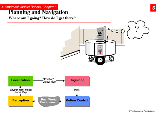
Autonomous Mobile Robots, Chapter 6
6.2.1
Road-Map Path Planning: Voronoi Diagram
• Easy executable: Maximize the sensor readings • Works also for map-building: Move on the Voronoi edges
© R. Siegwart, I. Nourbakhsh
Autonomous Mobile Robots, Chapter 6
6.2.1
Road-Map Path Planning: Adaptive Cell Decomposition
© R. Siegwart, I. Nourbakhsh
Autonomous Mobile Robots, Chapter 6
© R. Siegwart, I. Nourbakhsh
Autonomous Mobile Robots, Chapter 6
6.2.1
Road-Map Path Planning: Voronoi, Sysquake Demo
© R. Siegwart, I. Nourbakhsh
Autonomous Mobile Robots, Chapter 6
Ø Topological or metric or a mixture between both.
• First step:
Ø Representation of the environment by a road-map (graph), cells or a potential field. The resulting discrete locations or cells allow then to use standard planning algorithms.

自适应阈值Harris算法遥感图像配准的FPGA实现

第24期2023年12月无线互联科技Wireless Internet Science and TechnologyNo.24December,2023作者简介:汪强(1997 ),男,安徽宣城人,硕士研究生;研究方向:图像处理及FPGA 开发㊂自适应阈值Harris 算法遥感图像配准的FPGA 实现汪㊀强,郭来功(安徽理工大学电气与信息工程学院,安徽淮南232001)摘要:针对Harris 角点检测器响应值R 的阈值选择而导致角点失真问题,文章提出了一种基于现场可编程门阵列(FPGA )的自适应Harris 角点检测器实现遥感图像的配准方式㊂该方式依据非最大值抑制(NMS )处理后的响应值对阈值进行实时变化㊂实验结果显示,优化架构在硬件资源仅增加2.76%的情况下,准确率相应提升了8.31%㊂因此,文章提出的遥感图像配准架构适用于硬件资源有限的平台㊂关键词:Harris 角点检测器;FPGA ;非最大值抑制(NMS );遥感图像配准中图分类号:TP391㊀㊀文献标志码:A 0㊀引言㊀㊀在众多的计算机视觉应用中,Harris 角点检测被视为关键的预处理技术,例如特征识别㊁动态追踪㊁图像配准㊁3D 模型构建等㊂在众多常用的计算方法中,选择合适的阈值通常会对最终结果产生长远和深刻的影响㊂但是,在Harris 算法的应用中,阈值的选择只能依赖于个体的经验判断[1]㊂过高的阈值不仅可能导致角点信息的丢失,还可能引发伪角点的出现;较低的阈值不仅导致角点质量的下降,还会提高其对噪声的敏感性[2]㊂潘聪等[3]通过消除伪角点的方法,成功地实施了基于FPGA 的Harris 角点自适应阈值检测㊂本研究在其基础上,对自适应阈值算法进行了优化,并利用FPGA 将其成功应用于遥感图像配准技术中㊂1㊀Harris 角点检测算法㊀㊀在图像中,角点是正交轴渐变较高的点,Harris 算法能满足这些条件的点[4]㊂扫描窗口w (x ,y )(位移u 在x 方向,v 在y 方向),得到式(1):E (u ,v )=ðw (x ,y )[I (x +u ,y +v )-I (x ,y )]2(1)其中,w (x ,y )为(x ,y )处的窗口位置;I (x ,y )为(x ,y )处的强度;I (x +u ,y +v )为移动窗口(x +u ,y +v )处的强度㊂因为算法的最终目的是找到有角点(强度变化很大)的窗户㊂因此,必须最大化公式(1),则对公式(1)使用泰勒展开,得到公式(2):E (u ,v )=ð[I (x ,y )+uI x +vI y -I (x ,y )]2(2)展开公式(2),并用-I (x ,y )抵消I (x ,y ),得到公式(3):E (u ,v )=ðu 2I 2x+2uvI x I y +v 2I 2y(3)公式(3)可以用矩阵形式表示为:E (u ,v )=[u ㊀v ]ðw (x ,y )I 2xI x I y I x I y I 2y éëêêùûúú()u v éëêêùûúú(4)则公式(4)可表示为以下形式:E (u ,v )=[u ㊀v ]M u v éëêêùûúú(5)最后,计算遥感图像中每个窗口的分数,以确定其是否可能包含符合条件的角点:R =det (M )-k (trace (M ))2(6)其中,det (M )=λ1λ2;trace (M )=λ1+λ2㊂λ1和λ2相关数学意义如图1所示㊂在非最大抑制(NMS)中,如果半径r =1,则边界框为2ˑr +1=3㊂在这种情况下,考虑中心像素上的3ˑ3邻域㊂如果中心像素大于周围像素,则将其视为角点㊂同时将与半径内的周围像素进行比较㊂2㊀硬件实现架构㊀㊀遥感图像配准的硬件实现架构如图1所示,依次通过导数生成模块㊁高斯滤波模块㊁角点获得模块(角点提取和非最大值抑制)和优化后的自适应阈值模㊀㊀㊀㊀图1㊀λ1㊁λ2特征值相关数学意义块,以实现遥感图像角点的提取㊂至于图像配准部分,本次实验选择了特征法和区域法㊂2.1㊀导数生成模块㊀㊀导数生成器分别计算每一个像素水平方向和垂直方向的导数及其乘积[3]㊂先读取SDRAM存储器中图像灰度数据,再用IP核的加法器㊁减法器和乘法器来实现I2x㊁I2y和I x I y值的计算㊂其中,设置这3个数值的输出位宽为32㊂2.2㊀高斯滤波模块㊀㊀对上一步计算得到的3幅梯度图像进行高斯平滑处理,得到3个高斯值㊂高斯滤波模块窗口大小设置为3ˑ3,主要由X方向和Y方向进行㊂其中,图像在FPGA中是逐行输出的,因此需要通过延迟的方式来获得3ˑ3窗口内的9个图像像素值㊂其中实验输入的遥感图像大小为128ˑ128,对图像的第一二行分别进行128延迟和256延迟[5]㊂2.3㊀角点获得模块㊀㊀将高斯滤波得到的3个高斯值代入公式(7),得到遥感图像中每一个像素的Harris角点响应函数值R,其中R为该局部区域的最大值[6]㊂其计算需要完成3个乘法计算,并保存至寄存器中,其中乘以参数k (设k=0.06)的计算,使用算数右移来完成㊂同时避免造成角点团簇现象,R需要非最大值抑制(NMS),即去除一些较小值,将其中一些大于阈值的R输出进行后一级的角点配准功能[5]㊂2.4㊀自适应阈值模块㊀㊀阈值的选择对图像候选角点的质量也有很大影响㊂寻找理想阈值需要在未检测到的真角和检测到的假角之间进行权衡比较,这个阈值因图像而异[7]㊂本文设计的自适应模块结构如图2所示,依据NMS 后角点数量值N,分3个区间对阈值进行调节,同时利用简单地左右移1个单位以实现P值的乘除法,其中P取2.2ˑ10-7㊂图2㊀自适应阈值模块实现结构2.5㊀遥感图像配准模块㊀㊀特征法是通过图像中的特征点来进行图像的配准操作㊂核心的步骤包括:首先从2张图片中抽取特征点或描述特征的子项㊂再对2张图片中的特征点或描述子项进行匹配,以确定它们之间的匹配关系㊂依据所识别的相应关联,进行图像变换矩阵的计算㊂最后,对其中一张图像执行变换操作,确保2张图像在空间维度上达到配准状态㊂至于后2步通常采用最小二乘法来进行问题的解决,这样就可以达到图像的精确配准㊂3㊀仿真验证与分析㊀㊀该部分采用FPGA和MATLAB对比的方式进行㊂其中,FPGA采用Intel(Altera)公司CycloneⅣE系列的EP4CE15F23C6型开发平台,开发环境为Quartus II18.0,使用Verilog HDL完成数据流的描述㊂遥感图像配准仿真对比结果如图3 5所示㊂图3㊀传统遥感图像配准的MATLAB仿真4㊀结语㊀㊀本文提出的基于FPGA的自适应阈值Harris特征提取和遥感图像配准架构,以NMS为载体,改进自适应阈值模块,在FPGA占用资源增加2.76%的情况下,适度提高了遥感图像角点检测速度和配准精度㊂图4㊀传统遥感图像配准的FPGA仿真图5㊀自适应遥感图像配准的FPGA 仿真参考文献[1]孙万春.基于视频的公共场所人数统计研究[D ].重庆:重庆理工大学,2018.[2]孙万春,张建勋,朱佳宝,等.S -Harris :一种改进的角点检测算法[J ].重庆理工大学学报(自然科学),2018(10):156-161.[3]潘聪,黄鲁.基于FPGA 的自适应阈值Harris 角点检测硬件实现[J ].微型机与应用,2016(19):44-46,49.[4]SIKKA P ,ASATI A R ,SHEKHAR C.Real timeFPGA implementation of a high speed and areaoptimized Harris corner detection algorithm [J ].Microprocessors and Microsystems ,2021(2):1-6.[5]王跃霖.基于FPGA 的动态目标检测与跟踪系统的研究[D ].兰州:兰州交通大学,2018.[6]闫小盼,敖磊,杨新.Harris 角点检测的FPGA 快速实现方法[J ].计算机应用研究,2017(12):3848-3851.[7]MAURYA S ,CHOUDHURY Z ,PURINI S.Accuracyconfigurable FPGA implementation of Harris corner detection [C ].2022IEEE Computer Society Annual Symposium on VLSI (ISVLSI ).Nicosia ,2022:422-427.(编辑㊀沈㊀强)FPGA implementation of adaptive threshold Harris algorithm for remotesensing image registrationWang Qiang Guo LaigongSchool of Electrical and Information Engineering Anhui University of Technology Huainan 232001 ChinaAbstract Aiming at the problem of corner distortion caused by the threshold selection of the response value R ofHarris corner detector an adaptive Harris corner detector based on FPGA is proposed to achieve remote sensing imageregistration.This method changes the threshold in real -time based on the response value after Non Maximum Suppression NMS processing.The experimental results show that the optimized architecture achieved an accuracyimprovement of 8.31%with only a 2.76%increase in hardware resources.Therefore the remote sensing imageregistration architecture proposed in this article is suitable for computing on platforms with limited hardware resources.Key words Harris corner detector FPGA Non Maximum Suppression NMS remote sensing image registration。

基于自适应遗传算法的多无人机协同任务分配

2021,36(1)电子信息对抗技术Electronic Information Warfare Technology㊀㊀中图分类号:V279;TN97㊀㊀㊀㊀㊀㊀文献标志码:A㊀㊀㊀㊀㊀㊀文章编号:1674-2230(2021)01-0059-06收稿日期:2020-02-28;修回日期:2020-03-30作者简介:王树朋(1990 ),男,博士,工程师㊂基于自适应遗传算法的多无人机协同任务分配王树朋,徐㊀旺,刘湘德,邓小龙(电子信息控制重点实验室,成都610036)摘要:提出一种自适应遗传算法,利用基于任务价值㊁飞行航程和任务分配均衡性的适应度函数评估任务分配方案的优劣,在算法运行过程中交叉率和变异率进行实时动态调整,以克服标准遗传算法易陷入局部最优的缺点㊂将提出的自适应遗传算法用于多无人机协同任务分配问题的求解,设置并进行了实验㊂实验结果表明:提出的自适应遗传算法可以较好地解决多无人机协同任务分配问题,得到较高的作战效能,证明了该方法的有效性㊂关键词:遗传算法;适应度函数;无人机;任务分配;作战效能DOI :10.3969/j.issn.1674-2230.2021.01.013Cooperative Task Assignment for Multi -UAVBased on Adaptive Genetic AlgorithmWANG Shupeng,XU Wang,LIU Xiangde,DENG Xiaolong(Science and Technology on Electronic Information Control Laboratory,Chengdu 610036,China)Abstract :An improved adaptive genetic algorithm is proposed,and a fitness function based ontask value,flying distance and the balance of task allocation scheme is used to evaluate the qualityof task allocation schemes.In the proposed algorithm,the crossover probability and mutation prob-ability can adjust automatically to avoid effectively the phenomenon of the standard genetic algo-rithm falling into the local optimum.The proposed improved genetic algorithm is used to solve the problem of cooperative task assignment for multiple Unmanned Aerial Vehicles (UAVs).The ex-periments are conducted and the experimental results show that the proposed adaptive genetic al-gorithm can significantly solve the problem and obtain an excellent combat effectiveness.The ef-fectiveness of the proposed method is demonstrated with the experimental results.Key words :genetic algorithm;fitness function;UAV;task assignment;combat effectiveness1㊀引言无人机是一种依靠程序自主操纵或受无线遥控的飞行器[1],在军事科技方面得到了极大重视,是新颖军事技术和新型武器平台的杰出代表㊂随着战场环境日益复杂,对于无人机的性能要求越来越高,单一无人机在复杂的战场环境中执行任务具有诸多不足,通常多个无人机进行协同作战或者执行任务㊂通常地,多无人机协同任务分配是:在无人机种类和数量已知的情况下,基于一定的环境信息和任务需求,为多个无人机分配一个或者一组有序的任务,要求在完成任务最大化的同时,多个无人机任务执行的整体效能最大,且所付出的代价最小㊂从理论上讲,多无人机协同任务分配属于NP -hard 的组合优化问题,通常需95王树朋,徐㊀旺,刘湘德,邓小龙基于自适应遗传算法的多无人机协同任务分配投稿邮箱:dzxxdkjs@要借助于算法进行求解㊂目前,国内外研究人员已经对于多无人机协同任务分配问题进行了大量的研究,并提出很多用于解决该问题的算法,主要有:群算法㊁自由市场机制算法和进化算法等㊂群算法是模拟自然界生物群体的行为的算法,其中蚁群算法[2-3]㊁粒子群算法[4]以及鱼群算法[5]是最为典型的群算法㊂研究人员发现群算法可以用于求解多无人机协同任务分配问题,但是该算法极易得到局部最优而非全局最优㊂自由市场机制算法[6]是利用明确的规则引导买卖双方进行公开竞价,在短时间内将资源合理化,得到问题的最优解和较优解㊂进化算法适合求解大规模问题,其中遗传算法[7-8]是最著名的进化算法㊂遗传算法在运行过程中会出现不容易收敛或陷入局部最优的问题,许多研究人员针对该问题对遗传算法进行了改进㊂本文提出一种改进的自适应遗传算法,在算法运行过程中适应度值㊁交叉率和变异率可以进行实时动态调整,以克服遗传算法易陷入局部最优的缺点,并利用该算法解决多无人机协同任务分配问题,以求在满足一定的约束条件下,无人机执行任务的整体收益最大,同时付出的代价最小,得到较大的效费比㊂2㊀问题描述㊀㊀多无人机协同任务分配模型是通过设置并满足一定约束条件的情况下,包括无人机的自身能力限制和环境以及任务的要求等,估算各个无人机执行任务获得的收益以及付出的代价,并利用评价指标进行评价,以求得到最大的收益损耗比和最优作战效能㊂通常情况下,多无人机协同任务分配需满足以下约束:1)每个任务只能被分配一次;2)无人机可以携带燃料限制造成的最大航程约束;3)无人机载荷限制,无人机要执行某项任务必须装载相应的载荷㊂另外,多无人机协同任务分配需要遵循以下原则:1)收益最高:每项任务都拥有它的价值,任务分配方案应该得到最大整体收益;2)航程最小:应该尽快完成任务,尽可能减小飞行航程,这样易满足无人机的航程限制,同时降低无人机面临的威胁;3)各个无人机的任务负载尽可能均衡,通常以任务个数或者飞行航程作为标准判定; 4)优先执行价值高的任务㊂根据以上原则,提出多无人机协同任务分配的评价指标,包括:1)任务价值指标:用于评估任务分配方案可以得到的整体收益;2)任务分配均衡性指标:用于评估无人机的任务负载是否均衡;3)飞行航程指标:用于评估无人机的飞行航程㊂3㊀遗传算法㊀㊀要将遗传算法用于多无人机协同任务分配问题的求解,可以将任务分配方案当作种群中的个体,确定合适的染色体编码方法,利用按照一定结构组成的染色体表示任务分配方案㊂然后,通过选择㊁交叉和变异等遗传操作进行不断进化,直到满足约束条件㊂通常来说,遗传算法可以表示为GA=(C,E, P0,M,F,G,Y,T),其中C㊁E㊁P0和M分别表示染色体编码方法㊁适应度函数㊁初始种群和种群大小,在本文的应用中,P0和M分别表示初始的任务分配方案集合以及任务分配方案的个数;F㊁G 和Y分别表示选择算子㊁交叉算子和变异算子;T 表示终止的条件和规则㊂因此,利用遗传算法解决多无人机协同任务分配问题的主要工作是确定以上8个参数㊂3.1㊀编码方法利用由一定结构组成的染色体表示任务分配方案,将一个任务分配方案转换为一条染色体的过程可以分为2个步骤:第一步是根据各个无人机需执行的任务确定各个无人机对应的染色体;第二步是将这些小的染色体结合,形成整个任务分配方案对应的完整染色体㊂假设无人机和任务的个数分别为N u和N t,其中第i个无人机U i的06电子信息对抗技术㊃第36卷2021年1月第1期王树朋,徐㊀旺,刘湘德,邓小龙基于自适应遗传算法的多无人机协同任务分配任务共有k个,分别是T i1㊁T i2㊁㊁T ik,则该无人机对应的任务染色体为[T i1T i2 T ik]㊂在任务分配时,可能出现N t个任务全部分配给一个无人机的情况,另外为增加随机性和扩展性,提高遗传算法的全局搜索能力,随机将N t-k个0插入到以上的任务染色体中,产生一条全新的长度为N t的染色体㊂最终,一个任务分配方案可以转换为一条长度为N u∗N t的染色体㊂3.2㊀适应度函数在本文的应用中,适应度函数E是用于判断任务分配方案的质量,根据上文提出的多无人机协同任务分配问题的原则和评价指标可知,主要利用任务价值指标㊁任务分配均衡性指标以及飞行航程指标等三个指标判定任务分配方案的质量㊂假设有N u个无人机,F i表示第i个无人机U i的飞行航程,整个任务的总飞行航程F t可以表示为:F t=ðN u i=1F i(1)无人机的平均航程为:F=F t Nu(2)无人机飞行航程的方差D可以表示为:D=ðN u i=1F i-F-()2N u(3)为充分考虑任务价值㊁飞行航程以及各个无人机任务的均衡性,将任务分配方案的适应度函数定义为:E=V ta∗F t+b∗D(4)其中:V t为任务的总价值,F t为总飞行航程,D为各个无人机飞行航程的方差,a和b分别表示飞行航程以及飞行航程均衡性的权重㊂另外,任务分配方案的收益损耗比GL可以表示为:GL=V tF t(5)另外,在遗传算法运行的不同阶段,需要对任务分配方案的适应度进行适当地扩大或者缩小,新的适应度函数E可以表示为:Eᶄ=1-e-αEα=m tE max-E avg+1,m=1+lg T()ìîíïïïï(6)其中:E为利用公式(4)计算得到的原适应度值, E avg为适应度值的平均值,E max为适应度最大值,t 为算法的运行次数,T为遗传算法的终止条件㊂在遗传算法运行初期,E max-E avg较大,而t较小,因此α较小,可以提高低质量任务分配方案的选择概率,同时降低高质量任务分配方案的选择概率;随着算法的运行,E max-E avg将逐渐减小,t 将逐渐增大,因此α会逐渐增大,可以避免算法陷入随机选择和局部最优㊂3.3㊀种群大小㊁初始种群和终止条件按照通常做法,将种群大小M的取值范围设定为20~100㊂首先,随机产生2∗M个符合要求的任务分配方案,利用公式(4)计算各个任务分配方案的适应度值㊂然后,从中选取出适应度值较高的M 个任务分配方案组成初始种群P0,即初始任务分配方案集合㊂终止条件T设定为:在规定的迭代次数内有一个任务分配方案的适应度值满足条件,则停止进化;否则,一直运行到规定的迭代次数㊂3.4㊀选择算子首先,采用精英保留策略将当前适应度值最大的一个任务分配方案直接保留到下一代,提高遗传算法的全局收敛能力㊂随后,利用最知名的轮盘赌选择法选择出剩余的任务分配方案㊂3.5㊀交叉算子和变异算子在算法运行过程中需随时动态调整p c和p m,动态调整的原则如下:1)适当降低适应度值比平均适应度值高的任务分配方案的p c和p m,以保护优秀的高质量任务分配方案,加快算法的收敛速度;2)适当增大适应度值比平均适应度值低的任务分配方案的p c和p m,以免算法陷入局部最优㊂另外,任务分配方案的集中度β也是决定p c 和p m的重要因素,β可以表示为:16王树朋,徐㊀旺,刘湘德,邓小龙基于自适应遗传算法的多无人机协同任务分配投稿邮箱:dzxxdkjs@β=E avgE max(7)其中:E avg 表示平均适应度值;E max 表示最大适应度值㊂显然,β越大,任务分配方案越集中,遗传算法越容易陷入局部最优㊂因此,随着β增大,p c 和p m 应该随之增大㊂基于以上原则,定义p c 和p m 如下:p c =0.8E avg -Eᵡ()+0.6Eᵡ-E min ()E avg -E min +0.2㊃βEᵡ<E avg 0.6E max -Eᵡ()+0.4Eᵡ-E avg ()E max -E avg +0.2㊃βEᵡȡE avgìîíïïïïïp m =0.08E avg -E‴()+0.05E‴-E min ()E avg -E min +0.02㊃βE‴<E avg and β<0.80.05E max -E‴()+0.0001E‴-E avg ()E max -E avg+0.02㊃βE‴ȡE avg and β<0.80.5βȡ0.8ìîíïïïïïï(8)其中:E max 为最大适应度值,E min 为最小适应度值,E avg 为平均适应度值,Eᵡ为进行交叉操作的两个任务分配方案中的较大适应度值,E‴为进行变异操作的任务分配方案的适应度值,β为任务分配方案的集中度,可利用公式(7)计算得到㊂4㊀实验结果4.1㊀实验设置4架无人机从指定的起飞机场起飞,飞至5个任务目标点执行10项任务,最终降落到指定的降落机场㊂其中,如表1所示,无人机的编号分别为UAV 1㊁UAV 2㊁UAV 3和UAV 4㊂另外,起飞机场㊁降落机场㊁目标如图6所示㊂任务的编号分别为任务1至任务10(简称为T 1㊁T 2㊁㊁T 10),每项任务均为到某一个目标点执行侦察㊁攻击㊁事后评估中的某一项,任务设置如表2所示㊂表1㊀无人机信息编号最大航程装载载荷UAV 120侦察㊁攻击UAV 120侦察UAV 125攻击㊁评估UAV 130侦察㊁评估图1㊀任务目标位置示意图表2㊀任务设置任务编号目标编号任务类型任务价值T 11侦察1T 21攻击2T 32攻击3T 42评估3T 53侦察4T 63评估6T 74侦察2T 84攻击3T 94评估5T 105评估14.2㊀第一组实验首先,随机地进行任务分配,得到一个满足多无人机协同任务分配的约束条件的任务分配方案如下:㊃UAV 1:T 2ңT 5㊃UAV 2:T 1ңT 7㊃UAV 3:T 3ңT 6ңT 8㊃UAV 4:T 4ңT 9ңT 10计算可知,4个无人机的飞行航程分别是14.0674㊁12.6023㊁20.1854和22.1873,飞行总航程为69.0423,执行任务的总价值为30,最终的收益损耗比约为0.43㊂另外,各个飞行器飞行航程的方差约为16.18,UAV 1和UAV 2的飞行航程相对较短,而UAV 3和UAV 4的飞行航程相对较长,各个无人机之间的均衡性存在明显不足㊂为提高收益损耗比,分别利用标准遗传算法和本文提出的自适应遗传算法进行优化,两个算法的参数设置如表3所示㊂26电子信息对抗技术·第36卷2021年1月第1期王树朋,徐㊀旺,刘湘德,邓小龙基于自适应遗传算法的多无人机协同任务分配表3㊀遗传算法参数设置参数名称标准遗传算法自适应遗传算法E 公式(4)公式(6)M 2020选择方法精英策略轮盘赌选择法精英策略轮盘赌选择法P c 0.8公式(8)交叉方法单点交叉单点交叉P m 0.2公式(8)T500500最终,利用标准遗传算法得到任务分配方案如下:㊃UAV 1:T 3ңT 8㊃UAV 2:T 1ңT 7㊃UAV 3:T 9㊃UAV 4:T 6ңT 5计算可得,4个无人机的飞行航程分别为12.78㊁12.6023㊁12.434和12.9443,总飞行航程为50.7605,总任务价值为24,计算可知收益损耗比约为0.47,相对于随机任务分配提高约9.3%㊂另外,各个飞行器飞行航程的方差约为0.04,无人机飞行航程比较均衡,未出现飞行航程过长或过短的情况㊂在算法运行过程中,最佳适应度曲线如图2所示,在遗传算法约迭代到第160次时陷入局部最优,全局搜索能力不足㊂图2㊀标准遗传算法的最佳适应度曲线图1为进一步提高算法的效率,利用本文提出的改进自适应遗传算法解决多无人机协同任务分配问题㊂最终,利用自适应遗传算法得到的任务分配方案如下:㊃UAV 1:T 2ңT 3ңT 8ңT 7㊃UAV 2:T 5㊃UAV 3:T 6㊃UAV 4:T 1ңT 4ңT 9计算可知,4个无人机的飞行航程分别为12.8191㊁12.9443㊁12.9443和12.8191,总飞行航程为51.5268,总任务价值为29,收益耗比约为0.56,相对于随机任务分配提高约30.2%,相对于基于标准遗传算法的任务分配方案提高约19.1%㊂另外,各个飞行器飞行航程的方差约为0.004,无人机飞行航程的均衡性相对于基于标准遗传算法的任务分配方案有了进一步的提高㊂在算法运行过程中,最佳适应度值曲线如图3所示,可以有效避免遗传算法陷入局部最优或者随机选择㊂图3㊀自适应遗传算法的最佳适应度曲线图14.3㊀第二组实验在第一组实验中,因任务10(简称为T 10)的价值较低,在最终的任务分配方案中极少被分配㊂在第二组实验中,将T 10的价值由1调整为6,其他设置项不变㊂首先,随机进行任务分配,最终的任务分配方案和第一组实验相同㊂随后,利用标准遗传算法进行多无人机协同任务分配,最终的任务分配方案如下:㊃UAV 1:T 2ңT 3ңT 7ңT 8㊃UAV 2:T 5㊃UAV 3:T 6ңT 10㊃UAV 4:T 9基于此任务分配方案,4个无人机的飞行航程分别为12.8191㊁12.9443㊁13.6883和12.434,总飞行航程为51.8857,总任务价值为31,因此计36王树朋,徐㊀旺,刘湘德,邓小龙基于自适应遗传算法的多无人机协同任务分配投稿邮箱:dzxxdkjs@算可得收益损耗比约为0.6,相对于随机任务分配提高约17.6%㊂另外,各个飞行器飞行航程的方差约为0.21,各个无人机的飞行航程的均衡性一般,相对于随机任务分配有一定的提高㊂在算法运行过程中,最佳适应度值曲线如图4所示,在算法迭代运行约90次时陷入较长时间的局部最优,直到迭代次数为340次时,然后再次陷入局部最优㊂图4㊀标准遗传算法的最佳适应度曲线图2最后,将本文提出的自适应遗传算法用于多无人机协同任务分配问题的求解,得到最终的任务分配方案如下:㊃UAV 1:T 2ңT 3ңT 8ңT 7㊃UAV 2:T 5㊃UAV 3:T 6ңT 10㊃UAV 4:T 1ңT 4ңT 9基于此任务分配方案可得,4个无人机的航程分别是12.8191㊁12.9443㊁13.6883以及12.8191,总飞行航程为52.2708,总任务价值为35,计算可得效益损耗比约为0.67,相对于利用标准遗传算法得到的任务分配方案有了进一步提高㊂另外,各个无人机飞行航程的方差约为0.13,飞行航程的均衡性较好㊂在算法运行过程中,最佳适应度值曲线如图5所示,适应度值一直在实时动态变化,可以有效避免遗传算法陷入局部最优或者随机选择㊂由实验结果可得,当任务10的任务价值从1调整为6以后,不再出现该任务没有无人机执行的情况,这说明利用遗传算法进行多无人机协同任务分配可以根据任务的价值以及代价进行实时动态调整,符合优先执行价值高的任务的原则㊂图5㊀自适应遗传算法的最佳适应度曲线图25　结束语㊀㊀本文提出了一种基于自适应遗传算法的多无人机协同任务分配方法,整个遗传过程利用自适应的适应度函数评估任务分配结果的优劣,交叉率和变异率在算法运行过程中可以实时动态调整㊂实验结果表明,和随机进行任务分配相比,本文提出的方法在满足一定的原则和约束条件下,可以得到更高的收益损耗比,并且无人机飞行航程的均衡性更好㊂另外,和标准遗传算法相比,本文提出的改进遗传算法可以有效地扩展搜索空间,具有较高的全局搜索能力,不易陷入局部最优㊂参考文献:[1]㊀江更祥.浅谈无人机[J].制造业自动化,2011,33(8):110-112.[2]㊀楚瑞.基于蚁群算法的无人机航路规划[D].西安:西北工业大学,2006.[3]㊀杨剑峰.蚁群算法及其应用研究[D].杭州:浙江大学,2007.[4]㊀刘建华.粒子群算法的基本理论及其改进研究[D].长沙:中南大学,2009.[5]㊀李晓磊.一种新型的智能优化方法-人工鱼群算法[D].杭州:浙江大学,2003.[6]㊀AUSUBEL L M,MILGROM P R.Ascending AuctionsWith Package Bidding[J].Frontiers of Theoretical E-conomics,2002,1(1):1-42.[7]㊀刘昊旸.遗传算法研究及遗传算法工具箱开发[D].天津:天津大学,2005.[8]㊀牟健慧.基于混合遗传算法的车间逆调度方法研究[D].武汉:华中科技大学,2015.46。

Leuze电子扫描器说明书

Leuze electronic GmbH + Co. KG Post-box 1111 D-73277 Owen-Teck Tel. +49 7021 5730www.leuze.deW e r e s e r v e t h e r i g h t t o m a k e c h a n g e s • 96_d 06e .f mz Scanner with adjustable background suppressionz T wo switching pointsz Individual adaptation to applications by means of programming and diagnosis softwarez Universal sensor application through optional foreground suppression or exact edge detectionz General light/dark switching or complemen-tary switching output, scanning range adjustment and delay before start-up for optimal adaptation to the applicationz Robust metal housing with glass cover, pro-tection class IP 67/IP 69K for industrial application100…2500mm10 - 30 V DCAccessories:(available separately)z Mounting systems(BT 96, BT 96.1, BT 450.1-96, UMS 96)z Programming device UPG-2, Programming software z M12 connectors (KD …)z Ready-made cables (K-D…)Dimensioned drawingA B C D E F G H I Output with option switching delay K Connection terminals L Cable entryM Scanning range adjustment N Light/dark switchingPreferred entry direction for objects c +dElectrical connectionsee remarks !HRT 96Diffuse reflection light scanner with background suppressionHRT 96 M/P-1600-2000-42 - 05 HRT 96 M/P-3604-2000-42 - 05HRT 96 M/P-1600-2000-42 - 050603HRT 96 M/P-3604-2000-42 - 05SpecificationsDiagramsOptical dataHRT...1600...HRT...3604...Typ. scanning range limit (white 90%) 1)1)Typ. scanning range limit: max. attainable range without performance reserve 100…2500mm 10…2500mm Scanning range 2) 2)Scanning range: recommended range with performance reservesee tables see tables Adjustment range 150…2000mm 150…2000mm Light source LED (modulated light)Wavelength880nm TimingSwitching frequency 300Hz Response time1.67ms Delay before start-up≤200msElectrical dataOperating voltage U B 10…30VDC (incl. residual ripple)Residual ripple ≤15% of U B Bias current ≤35mASwitching outputPNP transistorFunction characteristics light/dark switching (reversible)Signal voltage high/low ≥(U B -2V)/≤2V Output current max.100mA IndicatorsSensor front LED green ready ready LED yellow reflection Sensor back LED red/greensee tablereflectionMechanical dataMetal housingHousing diecast zinc Optics cover glassWeight 380g Connection type terminals or M12 connector Environmental dataAmbient temp. (operation/storage)-20°C …+60°C/-40°C …+70°C Protective circuit 3)3)1=transient protection, 2=polarity reversal protection, 3=short circuit protection for all outputs, 4=interference blanking 1,2,3,4VDE safety class 4)4)Rating voltage 250VACII, all-insulated Protection class IP 67, IP 69K 5)5)IP 69K test acc. to DIN 40050 part 9 simulated, high pressure cleaning conditions without the use of additives, acids and bases are not part of the testLED class1 (acc. to EN 60825-1)Standards appliedIEC 60947-5-2OptionsSwitching delay (slow oper./release)0…10s (separately adjustable)-20-15-10-5051015200,511,522,53y1y2Distance x [m]M i s a l i g n m e n t y [m m ]Typ. response behaviour (white 90%)A white 90%B grey 18%C black 6%Scanning range x [m]R e d . o f s c a n r a n ge y [m m ]Typ. black/white behaviourOrder guideSelection tableOrder code ÎEquipment ÐH R T 96M /P -1600-2000-42P a r t N o . 500 60857H R T 96M /P -3604-2000-42P a r t N o . 500 60858Housing metalz z Light source infrared light (2000mm)z z Connection M12 connector zz Featuresshort rangez 2 switching points z switching delayz zcomplementary switching outputszTablesLight switchingDark switching z LED red/green:see Light switching z LED yellow:inverted1100200025002100199024703100198024301white 90%2grey 18%3black 6%Scanning range [mm]Typ. scanning range limit [mm]SwitchingpointsLED redLED green LED yellowno detection (reflection on background) on off off detection dis-tant range off on on detection close rangeonononRemarksz GeneralWith the set scanning range, a tolerance of the upper scan-ning range limit is possible de-pending on the reflection properties of the material sur-face.z Reference scannerScanner for safe detection of objects under most difficult environmental conditions (e.g. black object on white background).Is set through re-parameteri-sation of the standardHRT 96…3604… sensor via Software "Lupo".HRT 96…3604…z Switching pointsFixed ratio between short and distant ranges.r. ~0.5xd.r. Adjusting the distant range also sets the short range.z Switching outputPin/terminal4/3=distant range2/4=short range (standard)2/4=programmable(e.g. activation input, compl. switching output)HRT 96…1600…z Switching outputPin/terminal4/3=switching output2/4=compl. switching output z Available as a set together with cable socket KD 095HRT 96。

1、下载文档前请自行甄别文档内容的完整性，平台不提供额外的编辑、内容补充、找答案等附加服务。
2、"仅部分预览"的文档,不可在线预览部分如存在完整性等问题,可反馈申请退款(可完整预览的文档不适用该条件!)。
3、如文档侵犯您的权益，请联系客服反馈,我们会尽快为您处理(人工客服工作时间：9:00-18:30)。

∗ in: Proceedings of International Panel Conference on Soft and Intelligent Computing, Technical University of Budapest, 1996 43-50. † Presently visiting professor at Institute for Advanced Management Systems Research, ˚ Abo Akademi University. Partially supported by OTKA T 14144
Keywords: hyperknowledge support system, approximate reasoning, cognitive map, error correction learning, strategic management.
1
Woodstrat project
Strategic Management is deﬁned as a system of action programs which form sustainable competitive advantages for a corporation, its divisions and its business units in a strategic planning period. A research team of the IAMSR institute has developed a support system for strategic management, called the Woodstrat, in two major Finnish forest industry corporations in 1992-96. The system is modular and is built
1
around the actual business logic of strategic management in the two corporations, i.e. the main modules cover the market position (MP), the competitive position (CP), the productivity position (PROD), the proﬁtability (PROF) , the investments (INV) and the ﬁnancing of investments (FIN). The innovation in Woodstrat is that these modules are linked together in a hyperknowledge fashion, i.e. when a strong market position is built in some market segment it will have an immediate impact on proﬁtability through links running from key assumptions on expected developments to the projected income statement. There are similar links making the competitive position interact with the market position, and the productivity position interact with both the market and the competitive positions, and with the proﬁtability and ﬁnancing positions.
Adaptive Fuzzy Cognitive Maps for Hyperknowledge Representation in Strategy Formation Process ∗
Christer Carlsson IAMSR, ˚ Abo Akademi University, DataCity A 3210, SF-20520 ˚ Abo, Finland e-mail: ccarlsso@ra.abo.ﬁ Robert Full´ er † Comp. Sci. Dept., E¨ otv¨ os Lor´ and University, Muzeum krt. 6-8, H-1088 Budapest, Hungary e-mail: rfuller@ra.abo.ﬁ
2
Hyperknowledge and Cognitive Maps
Hyperknowledge is formed as a system of sets of interlinked concepts [9], much in the same way as hypertext is built with interlinked text strings [16]; then hyperknowledgefunctions would be constructs which link concepts/systems of concepts in some predetermined or wanted way. There are some useful characteristics of a hyperknowledge environment [9]: (i) the user can navigate through and work with diverse concepts; (ii) concepts can be diﬀerent epistemologically, (iii) concepts can be organized in cognitive maps, (iv) 2
MP
CP
PROF
INV
FI N
Fig. 2ts of the strategy building process.
Figure 1
The framework of Woodstrat.
The Woodstrat oﬀers an intuitive and eﬀective strategic planning support with object-oriented expert systems elements and a hyperknowledge user interface. In this paper we will show that the eﬀectiveness and usefulness of a hyperknowledge support system can be further advanced using adaptive fuzzy cognitive maps.
Abstract In [6] Carlsson demonstrated that all the pertinent conceptual constructs of strategic management theory can be represented with a knowledge based support (KBS)-system with hyperknowledge properties. Furthermore, he shows that cognitive maps can be used to trace the impact of the support and to generalize the experiences of the users. In this paper we will show that the eﬀectiveness and usefulness of this hyperknowledge support system can be further advanced using adaptive fuzzy cognitive maps.
the concepts can be made interrelated and interdependent, (v) relations can be structured or dynamic, and (vi) relations can change with or adapt to the context. Cognitive maps were introduced by Axelrod [1] to represent crisp cause-eﬀect relationships which are perceived to exist among the elements of a given environment. Fuzzy cognitive maps (FCM) are fuzzy signed directed graphs with feedbacks, and they model the world as a collection of concepts and causal relations between concepts [12]. When addressing strategic issues cognitive maps are used as action-oriented representations of the context the managers are discussing. They are built to show and simulate the interaction and interdependences of multiple belief systems as these are described by the participants - by necessity, these belief systems are qualitative and will change with the context and the organizations in which they are developed. They represent a way to make sure, that the intuitive belief that strategic issues should have consequences and implications, that every strategy is either constrained or enhanced by a network of other strategies, can be adequately described and supported. For simplicity, in this paper we illustrate the strategy building process by the following fuzzy cognitive map with six states