Mapping soil salinity in the Yangtze delta REML and universal kriging E-BLUP revised
土壤问题作文英语

土壤问题作文英语In recent years, soil has become a focal point of environmental concern due to its critical role in supporting life on Earth. The essay will delve into the various issues that are currently affecting our soil, the consequences of these problems, and potential solutions to mitigate them.Soil DegradationSoil degradation is a widespread problem that encompasses erosion, salinization, and nutrient depletion. The excessive use of chemical fertilizers and pesticides has led to soil acidification and the loss of organic matter, which are detrimental to soil health and fertility.ErosionErosion is the process by which soil is worn away, primarily by water and wind. It is exacerbated by deforestation and poor agricultural practices, leading to the loss of topsoil, which is rich in nutrients and essential for plant growth.SalinizationSalinization occurs when salts accumulate in the soil, making it unsuitable for plant growth. This is often a result of irrigation practices that do not adequately drain the water, leading to a buildup of salts in the soil profile.Nutrient DepletionContinuous cultivation without adequate replenishment of nutrients can lead to nutrient depletion. This results in soils that are unable to support plant life, leading to reduced crop yields and food insecurity.ConsequencesThe consequences of soil issues are far-reaching. They include reduced agricultural productivity, loss of biodiversity, and increased vulnerability to natural disasters such as floods and droughts. Moreover, degraded soils contribute to climate change by releasing stored carbon into the atmosphere.SolutionsTo address these soil issues, several strategies can be implemented. Sustainable farming practices, such as crop rotation, organic farming, and conservation tillage, can help maintain soil health. Additionally, reforestation efforts can reduce erosion and improve water retention. Government policies and regulations can also play a crucial role in promoting sustainable land management practices.ConclusionSoil is a non-renewable resource that requires careful management to ensure its long-term viability. Byunderstanding and addressing the issues of soil degradation, erosion, salinization, and nutrient depletion, we can work towards a more sustainable future that supports both human needs and the health of our planet.。
土壤沙化的英文作文
土壤沙化的英文作文Soil desertification is a serious environmental issue that affects many regions around the world. It occurs when the soil loses its fertility and becomes dry and sandy, making it difficult for plants to grow.The main causes of soil desertification include overgrazing, deforestation, and improper agricultural practices. When these activities are carried out without proper management, they can lead to the degradation of the soil and the loss of its ability to support plant life.One of the consequences of soil desertification is the loss of biodiversity. As the soil becomes less fertile, many plant species are unable to survive, leading to a decrease in the overall diversity of plant life in the affected area.In addition to impacting plant life, soil desertification also has negative effects on the localeconomy. Farmers may struggle to grow crops in degraded soil, leading to lower yields and decreased income. This can have a ripple effect on the entire community, as people may struggle to access food and other resources.Efforts to combat soil desertification include implementing sustainable land management practices, reforestation, and soil conservation techniques. By taking action to protect and restore the soil, we can help prevent further degradation and ensure a healthier environment for future generations.。
土壤盐渍化的原因英文作文500字

土壤盐渍化的原因英文作文500字英文回答:Soil salinization is the process by which soluble salts accumulate in the soil, often to the detriment of plant growth. It is a major environmental problem, affecting over 950 million hectares of land worldwide, and is expected to worsen in the future due to climate change and increased water scarcity.There are two main types of soil salinization:Primary salinization: This occurs when salt-laden water evaporates from the soil, leaving behind the salts. This can happen naturally in arid and semi-arid regions, where the evaporation rate exceeds the precipitation rate. It can also be caused by human activities, such asirrigation with saline water or the clearing of forests, which can lead to increased evaporation.Secondary salinization: This occurs when salts are brought to the surface by capillary action or by the rising water table. This can happen naturally in areas with a high water table, or it can be caused by human activities, such as the construction of dams or the over-extraction of groundwater.Soil salinization can have a number of negative effects on plant growth, including:Reduced water uptake: Salts can interfere with the plant's ability to absorb water from the soil.Reduced nutrient uptake: Salts can also interfere with the plant's ability to absorb nutrients from the soil.Toxicity: High levels of salts can be toxic to plants, causing damage to the roots, stems, and leaves.Soil salinization can also have a number of negative effects on the environment, including:Loss of biodiversity: Soil salinization can lead to the loss of plant and animal species, as well as the disruption of ecosystem services.Degradation of water quality: Soil salinization can lead to the contamination of surface and groundwater with salts.Desertification: Soil salinization can lead to the desertification of land, making it uninhabitable for humans and other animals.There are a number of ways to prevent and mitigate soil salinization, including:Reducing irrigation with saline water: Using saline water for irrigation can lead to the accumulation of salts in the soil. Reducing the amount of saline water used for irrigation can help to prevent soil salinization.Improving drainage: Improving drainage can help to prevent the rise of the water table and the accumulation ofsalts in the soil.Planting salt-tolerant crops: Planting salt-tolerant crops can help to reduce the negative effects of soil salinization.Using gypsum: Gypsum is a mineral that can help to reduce the salinity of the soil. It can be applied to the soil to help remove salts.Soil salinization is a major environmental problem, but it can be prevented and mitigated through the use of appropriate management practices.中文回答:土壤盐渍化的原因。
土壤盐渍化的原因英文作文500字
土壤盐渍化的原因英文作文500字Soil salinization has become a severe global issue affecting agricultural productivity and ecosystem sustainability. Understanding its causes is crucial for developing effective mitigation and management strategies.In this essay, we will delve into the primary factors contributing to soil salinization.1. Natural Processes:a. Tectonic Activity: The uplift of certain geological formations, such as salt domes and ancient marine sediments, can bring salt-laden rocks close to the soil surface. Over time, weathering and erosion release these salts into the soil profile.b. Mineral Weathering: The weathering of certain minerals, such as pyrite and gypsum, can liberate soluble salts that accumulate in the soil. Pyrite oxidation, in particular, produces sulfuric acid, further exacerbatingsalinization.c. Atmospheric Deposition: Sea spray, volcanic eruptions, and dust storms can deposit salt particles into the soil. In coastal areas, salt deposition from ocean spray is a significant contributor to soil salinization.2. Human Activities:a. Irrigation: Over-irrigation is a major anthropogenic cause of soil salinization. When excess water is applied to soil, it dissolves and transports salts from deeper layers to the surface. As the water evaporates, these salts accumulate in the topsoil, increasing its salinity.b. Poor Drainage: Inadequate drainage systems allow water to stagnate in the soil, promoting the accumulation of salts. Poor soil permeability, high water tables, and excessive watering can lead to waterlogging and subsequent salinization.c. Deforestation: The removal of vegetation cover,particularly in arid and semi-arid regions, can disrupt the natural water cycle and increase soil evaporation rates. This leads to the concentration of salts in the topsoil, as water evaporates and leaves behind dissolved solids.d. Fertilization: The excessive application of certain fertilizers, especially those containing high levels of soluble salts, can contribute to soil salinization. Synthetic fertilizers, such as ammonium sulfate and potassium chloride, can release significant amounts ofsalts when applied in excessive quantities.3. Climate Change:a. Rising Sea Levels: In coastal areas, rising sea levels can lead to the intrusion of saltwater into freshwater aquifers and soil profiles. This saltwater intrusion increases the salinity of the soil, affecting plant growth and ecosystem health.b. Changes in Precipitation Patterns: Climate change can alter precipitation patterns, leading to more frequentand intense droughts or floods. These extreme events can exacerbate soil salinization through reduced water availability or increased salt deposition.c. Temperature Rise: Higher temperatures can increase the rate of evaporation, which in turn can concentratesalts in the topsoil. This is especially concerning in arid and semi-arid regions where water scarcity is already a challenge.Understanding the causes of soil salinization is essential for developing tailored management strategies. To mitigate the impact of natural processes, proper irrigation practices, adequate drainage systems, and sustainable land-use planning are crucial. Human activities can be regulated through responsible water use, efficient fertilizer application, and the promotion of sustainable agricultural practices. Climate change adaptation measures, such as improved drought tolerance in crops and the development of salt-tolerant plant varieties, are becoming increasingly important. By addressing the root causes of soil salinization, we can work towards preserving theproductivity of agricultural lands and safeguarding the health of ecosystems around the world.。
西南黄海2018年夏季溶解氧分布特征及其影响因素的初步分析
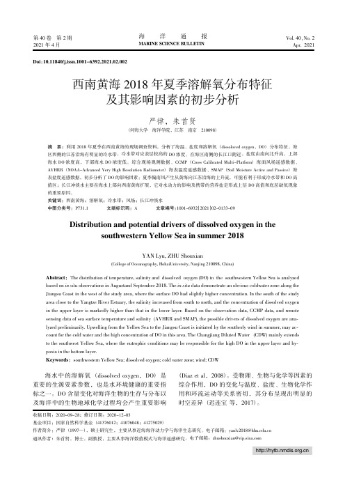
西南黄海2018年夏季溶解氧分布特征及其影响因素的初步分析严律,朱首贤(河海大学海洋学院,江苏南京210098)摘要:利用2018年夏季在西南黄海的现场调查资料,分析了海温、盐度和溶解氧(dissoloved oxygen ,DO)分布特征。
海区西侧的江苏沿海有明显的冷水带,冷水带对应表层较高的DO 浓度。
在海区南侧的长江口附近,盐度由南向北升高,上部海水DO 浓度高,下部海水DO 浓度低。
综合现场观测数据、CCMP (Cross Calibrated Multi-Platform )海面风场遥感数据、AVHRR (NOAA-Advanced Very High Resolution Radiometer )海表温度遥感数据、SMAP (Soil Moisture Active and Passive)海表盐度遥感数据,初步分析了DO 的影响因素:夏季偏南风产生从黄海向江苏沿海的上升流,可能有利于形成冷水带和DO 高值区;长江冲淡水主要在海水上部向西南黄海扩展,它对水动力的影响及携带的营养盐是形成上层DO 高值和底层缺氧现象的重要原因。
关键词:西南黄海;溶解氧;冷水带;风场;长江冲淡水中图分类号:P731.1文献标识码:A文章编号:1001原6932(圆园21)02原园133原09收稿日期:2020-09-28;修订日期:2020-12-03基金项目:国家自然科学基金(41376012;41076048;41275029)作者简介:严律(1997—),硕士研究生,主要从事近海海洋动力学与海洋生态研究。
电子邮箱:*****************.cn通讯作者:朱首贤,博士,副教授,主要从事海洋数值模式与海洋遥感研究。
电子邮箱:********************.comDistribution and potential drivers of dissolved oxygen in thesouthwestern Yellow Sea in summer 2018YAN Lyu,ZHU Shouxian(College of Oceanography,HohaiUniversity,Nanjing 210098,China)Abstract :The distribution of temperature,salinity and dissolved oxygen (DO)in the southwestern Yellow Sea is analyzed based on in situ observations in Augustand September 2018.The in situ data demonstrate an obvious coldwater zone along the Jiangsu Coast in the west of the study area,where the surface DO had slightly higher concentration.In the south of the study area close to the Yangtze River Estuary,the salinity increased from south to north,and the concentration of dissolved oxygenin the upper layer is markedly higher than that in the lower layer.Based on the observation data,CCMP data,and remote sensing data of sea surface temperature and salinity (AVHRR and SMAP),the possible drivers of dissolved oxygen are ana鄄lyzed preliminarily.Upwelling from the Yellow Sea to the Jiangsu Coast is initiated by the southerly wind in summer,may ac鄄count for the cold water and the high concentration of DO in this area.The Changjiang Diluted Water (CDW)mainly extendsto the southwest Yellow Sea,where the eutrophic conditions may be responsible for the high DO in the upper layer and hy鄄poxia in the bottom layer.Keywords :southwestern Yellow Sea;dissolved oxygen;cold water zone;wind;CDW海水中的溶解氧(dissolved oxygen ,DO )是重要的生源要素参数,也是水环境健康的重要指标之一。
海洋勘探英文作文

海洋勘探英文作文Title: Exploring the Depths: Oceanic Exploration。
Oceanic exploration stands at the forefront of scientific discovery, unveiling mysteries hidden beneath the waves. From the vast expanse of the sea floor to the intricate ecosystems thriving in its depths, the exploration of the ocean holds immense importance for understanding our planet's past, present, and future.First and foremost, oceanic exploration provides invaluable insights into Earth's geology and tectonic activity. Through technologies like sonar mapping and seismic surveys, scientists can unravel the complex structures of underwater mountain ranges, trenches, and volcanoes. These efforts not only contribute to our understanding of plate tectonics but also help assess geological hazards such as earthquakes and tsunamis, enhancing our ability to mitigate their impact on coastal communities.Furthermore, the exploration of the ocean plays a crucial role in studying climate patterns and their effects on marine ecosystems. Oceanographers monitor sea surface temperatures, currents, and salinity levels to track changes in ocean circulation and climate dynamics. By analyzing sediment cores and studying ancient coral reefs, researchers can reconstruct past climate conditions, offering valuable insights into long-term climate trends and the potential impacts of climate change.Moreover, oceanic exploration supports biodiversity conservation by uncovering new species and habitats that are vital to marine ecosystems. Deep-sea expeditions reveal astonishing creatures adapted to extreme pressures and darkness, from bioluminescent jellyfish to elusive giant squids. By documenting these species and their habitats, scientists can advocate for their protection and contribute to the preservation of marine biodiversity.In addition to scientific research, oceanic exploration holds significant economic potential through the discoveryof valuable resources and the development of marine industries. Deep-sea mining operations seek to extract minerals such as manganese, cobalt, and rare earth elements from the ocean floor, which are essential for modern technologies like smartphones and electric vehicles. However, these activities must be conducted sustainably to minimize environmental damage and protect fragile marine ecosystems.Furthermore, oceanic exploration contributes to the sustainable management of fisheries by providing data on fish stocks, migration patterns, and ecosystem dynamics. By understanding the interconnectedness of marine species and their habitats, policymakers can implement effective conservation measures to prevent overfishing and preserve the health of marine ecosystems for future generations.In conclusion, oceanic exploration plays a vital rolein advancing scientific knowledge, promoting environmental stewardship, and driving economic development. By continuing to explore the depths of the ocean withcuriosity and diligence, we can unlock its secrets andharness its resources in a responsible and sustainable manner.。
土地利用监测与精明增长翻译
在美国各地的社区投入更多的时间,注意力和精力来管理土地的使用以适应不断扩大的人口或其他增长压力,许多人发现他们缺乏做的扎实的远景规划的基本信息。
大多数人认为增长管理是一把双刃剑:如果社区开放太多的土地以供开发,由此产生的扩展可能是付出昂贵的环境,社会和经济上的代价。
但如果他们太严格限制土地可供开发,需求可能很快超过供应,迫使土地和住房价格大幅上涨。
为平衡上述问题,在土地管理工作方面需要做出的努力是:社区需要一种方法来监测当前土地的使用状况,评估未来的需求,并采取措施确保未来充足的土地供应。
幸运的是,现在有性价比高,可用于几乎任何社区实施土地监测的方便的工具。
这样做很快发现,这样的系统可以成为综合智慧增长规划的一个重要工具。
平衡相互竞争的住房,商业和环境保护的用地需求给社区官员提出了困难的,也是日常的挑战。
在智慧增长语境下,解决这些相关问题使这些挑战变得更加复杂。
近年来,众多的组织和学术界成员都阐述了实施精明增长的重要性如遵循提供足量老百姓可以获得的房屋(经适房),保护自然资源和内涵城市增长(containing urban growth)原则。
美国环境保护局,城市土地研究所,全国住宅建筑商协会,和美国规划协会等不同组织都声称支持这些观念。
大多数社区普遍认为精明增长目标值得称赞,但他们经常发现他们缺乏必要的工具来做出老道明智的、能经受住时间考验的土地利用决策。
在许多社区依据“精明增长”形成了遏制城市增长的政策。
如前面所指出的,一个微妙的平衡,是要求这些政策取得成功。
太少的容纳式城市增长原则是鼓励城市蔓延的,并且太多容纳式(containment)增长引起了土地和房屋价格的通胀。
这一困境使得社区去规划满足未来的住房需求尤其困难,而这恰恰是社区必须提供的最重要的功能。
根据最近发布的报告表示,住房提供了超过三分之一的国家的有形资产及以以及房主50%的净资产。
研究表明,那些生活在稳定社区的家庭的孩子更容易完成学业,且有有更好的学习成绩和较少的行为问题。
农田变成沙土英语作文
农田变成沙土英语作文英文回答:Agricultural land transitioning into sandy soil is a pressing issue with far-reaching implications. Factors contributing to this phenomenon include:Soil erosion: Deforestation, overgrazing, and improper agricultural practices accelerate soil erosion, leading to the loss of nutrient-rich topsoil and accumulation of sand.Climate change: Rising temperatures and altered precipitation patterns exacerbate soil erosion, especiallyin arid and semi-arid regions where moisture scarcity promotes wind erosion.Irrigation mismanagement: Excessive or poorly timed irrigation practices can leach away valuable soil particles, leaving behind lighter, sandy material.Soil compaction: Heavy machinery and excessive livestock grazing compress soil, reducing its water infiltration capacity and increasing its vulnerability to wind erosion.Deforestation: Trees play a crucial role in soil stabilization. Their roots bind soil particles and reduce wind velocity, preventing soil loss. Deforestation disrupts this protective mechanism.Consequences of sandy soil include:Reduced soil fertility: Sandy soil lacks the nutrients and organic matter necessary for optimal plant growth.Increased susceptibility to drought: Sand has poor water-holding capacity, leading to rapid water loss and reduced crop yields.Difficulty in nutrient uptake: Sandy soil particles do not bind nutrients as effectively as clay particles, making it difficult for plants to access essential nourishment.Erosion susceptibility: Sandy soil is easily eroded by wind and water, exacerbating land degradation.Reduced agricultural productivity: Sandy soil hinders plant growth and reduces crop yields, threatening food security.Mitigation strategies include:Conservation agriculture: Adopting sustainable farming practices that minimize soil erosion, such as no-till farming and cover cropping.Reforestation: Planting trees to stabilize soils, reduce wind erosion, and improve water infiltration.Improved irrigation practices: Using efficient irrigation methods and applying water at appropriate intervals to prevent soil leaching.Soil amendment: Adding organic matter, such as compostor manure, to sandy soil to improve its fertility and water retention capacity.Erosion control measures: Implementing erosion control structures, such as terraces and windbreaks, to reduce soil loss.中文回答:农田沙化现象。
- 1、下载文档前请自行甄别文档内容的完整性,平台不提供额外的编辑、内容补充、找答案等附加服务。
- 2、"仅部分预览"的文档,不可在线预览部分如存在完整性等问题,可反馈申请退款(可完整预览的文档不适用该条件!)。
- 3、如文档侵犯您的权益,请联系客服反馈,我们会尽快为您处理(人工客服工作时间:9:00-18:30)。
Mapping soil salinity in the Yangtze delta:REML and universal kriging (E-BLUP)revisitedH.Y.Li a ,b ,c ,R.Webster b ,Z.Shi c ,⁎a School of Tourism and Urban Management,Jiangxi University of Finance and Economics,Nanchang 330013,Chinab Rothamsted Research,Harpenden AL52JQ,Great Britain,UKcCollege of Environmental and Resource Sciences,Zhejiang University,Hangzhou 310058,Chinaa b s t r a c ta r t i c l e i n f o Article history:Received 17February 2014Received in revised form 19May 2014Accepted 21August 2014Available online xxxx Keywords:Saline soilElectrical conductivity Trend surface analysis REMLUniversal kriging E-BLUPRice farmers in China need accurate maps of soil salinity to make rational decisions for management.Modern sensors such as the Geonics EM38conductivity meter,which records the apparent electrical conductivity,EC a ,allied to geostatistics to convert sparse punctual measurements into digital maps can provide them.We have explored the combination in reclaimed land in the Hangzhou Gulf of the Yangtze delta in Zhejiang Prov-ince in south-east China.The EC a was measured at 525points in a 2.2-ha field that was reclaimed in 1996.The data,transformed to logarithms,were treated as the realization of a mixture of strong quadratic trend and corre-lated random residuals.We estimated the coef ficients of the trend and the parameters of the covariance of the residuals by residual maximum likelihood (REML).We then kriged the log 10EC a on to a fine grid by universal kriging (UK),and transformed the predictions back to EC a for mapping.For comparison we also include regres-sion kriging using the estimated variogram of the ordinary least squares residuals from the trend.We compared the results by cross-validation and calculated the mean errors (MEs),mean squared errors (MSEs)and mean squared deviation ratios (MSDRs).All combinations of technique gave small MEs,as expected —kriging is unbiased.The MSEs varied somewhat.The MSDRs,which ideally should equal 1,varied more.The combination with an MSDR closest to 1was UK with the spherical variogram estimated by REML;its MSDR was 0.993.We matched the predictions to the US Department of Agriculture ’s classes of soil salinity and found that approx-imately half of the field fell into its slightly saline and moderately saline classes,where rice yields would yield a pro fit to the farmer,and half were in the very saline and extremely saline classes where rice yields were so poor that the farmer would lose money by attempting to grow rice.©2014Elsevier B.V.All rights reserved.1.IntroductionDuring the past 40years,more than 400000ha of the tidelands in the Yangtze delta of China has been reclaimed for agriculture (Huang et al.,2008).When first enclosed the soil is saline,and most of the salt must be leached away before the land can be used to grow rice.Barley,wheat and cotton are more tolerant of salt,but they are less pro fitable.Farmers have relied on their experience to decide when to plant rice,but often their crops have failed because the soil was still too nd managers therefore want accurate estimates of the soil ’s salinity in map form so that they can judge when and where they can success-fully grow rice (Li et al.,2013).Fortunately,modern proximal soil sensors based on electromagnetic induction (EM)such as the EM31and EM38(McNeill,1980)enable man-agers or their advisors to measure the soil ’s apparent electrical conductiv-ity (EC a )fairly quickly from above the ground surface.The technique is now widely used in surveys of soil salinity (Akramkhanov et al.,2014;Guo et al.,2013;Trianta filis et al.,2013).Even so,the data from the instru-ments are effectively at points in the field with more or less large dis-tances between them.Interpolation is usually necessary for mapping,and nowadays kriging is used for the purpose.For example,for our earlier paper (Li et al.,2013)we had recorded the EC a at only 56points from which to map a field of 2.22ha.In a more recent survey of the field we made 525observations,and these revealed a strong trend;we describe the detail below.De Clercq et al.(2009)and Akramkhanov et al.(2014)also encountered strong trends when mapping soil salinity.Ordinary kriging,the familiar ‘workhorse ’of geostatistics and now readily accessible in computer packages,is based on the assumption that the variable of interest is intrinsically stationary.If there is trend,however,the assumption is untenable,and a more elaborate model of the variation is needed to take into account the trend.The trend might also be of interest in its own right and not simply be a nuisance.Matheron (1969)introduced what he called ‘universal kriging ’to deal with the situation.It is based on the model:Z x ðÞ¼u x ðÞþεx ðÞ:ð1ÞGeoderma 237–238(2015)71–77⁎Corresponding author.E-mail address:shizhou@ (Z.Shi)./10.1016/j.geoderma.2014.08.0080016-7061/©2014Elsevier B.V.All rightsreserved.Contents lists available at ScienceDirectGeodermaj o ur n a l h o m e p a g e :w ww.e l s e v i e r.c o m/l o c a t e /g e o de r m aIn this model u (x )is a non-stationary mean at place x representing the trend,and ε(x )is a stationary random residual with zero mean and covariance function or variogram (h ).The trend is typically treated as a low-order polynomial function of x ,f (x ),linear,quadratic or cubic.Matheron ’s technique requires a model for that variogram,but Matheron did not say how to estimate it.The problem is that until one knows the trend one cannot derive a valid model for the variogram,and without that model one cannot estimate the trend correctly.Various attempts have been made to get round this impasse.Olea (1975)devised an algo-rithm for data on regular grids.Another approach,recommended by Goovaerts (1997)and applied by Meul and Van Meirvenne (2003),is to compute and model the variogram perpendicular to a dominant trend.Neither technique is general,however.Regression kriging in which the interdependence of the trend and variation in the residuals is disregarded enjoys some popularity.Its pre-dictions are unbiased,but the prediction variances underestimate the true prediction errors,often seriously (Lark and Webster,2006);see Lark et al.(2006)and Webster and Oliver (2007)for an explanation.Minasny and McBratney (2007)make the point that its bias decreases as the number and density of data increase,and it might be the only feasible technique for handling the very large numbers of data from proximal sensors ‘on the run ’.Stein (1999)drew geostatisticians ’attention to likelihood methods,though the first statistician to recommend them seems to have been Kitinidis (1983,1993)with what he called ‘generalized covariance func-tions ’,from which any trend has been removed.The latter ’s approach is effectively that of residual (or restricted)maximum likelihood (REML),originally devised by Patterson and Thompson (1971)for estimating components of variance.The method estimates both the trend coef fi-cients and the covariance of the residuals simultaneously.The two are then combined with the data to provide empirical best linear unbiased predictions (E-BLUP)(Lark et al.,2006;Minasny and McBratney,2007).Once a covariance function has been estimated in this way E-BLUP pro-duces the same predictions as universal kriging does with that function (Stein,1999).This method is quite feasible for the few hundreds of data that accrue typically from laboratory measurements and static sensors.It is now regarded as best practice,and it is the one we use here to explore the variation in salinity in the Yangtze delta.2.Site and Methods 2.1.Study Area and SamplingThe land in the coastal zone of Zhejiang Province south of HangzhouGulf of the Yangtze delta is formed of recent marine and fluvial deposits.The soil consists predominantly of uniform pro files of light loam orsandy loam textures,with a sand content of about 60%.It is also saline,with large concentrations of Na and Mg salts (in many places N 1%).The climate is subtropical with an average temperature of 16.5°C and a mean annual rainfall of 1300mm.During the past 30years much of this zone has been enclosed and reclaimed for agriculture.The fields we describe below were reclaimed in 1996and were first used to produce irrigated cotton.Since 2006these fields have been farmed for paddy rice.However,whilst reclama-tion has been fairly successful,salinity is now increasing,and countering it is becoming problematic.Means are required to measure and monitor the dynamics of salinization so that the land can be managed for rice.To test the ability of the EM38to provide the necessary information we chose to study a field approximately 2.2ha.The fields lie to the north of Shangyu City at 30°9′N,120°48′E (Fig.1).We measured the EC a with a Geonics EM38conductivity meter with the coils con figured vertically at 525points,fairly evenly spread in the field.We did so after the rice had been harvested.Each position was georeferenced by a Trimble Global Positioning System.Fig.2is a ‘bubble plot ’of the data with ‘bub-bles ’,i.e.circles or discs,of diameter proportional to the measured values.Table 1summarizes the statistics of the data.2.2.Trend Surface Analysis and Interpolation by Ordinary Kriging The bubble plot (Fig.2)shows a zone of large values towards the south-east of the region.The pattern seems to have the general form of a quadratic trend surface,and we therefore fitted such a surface ini-tially by ordinary least squares (OLS)regression.The model expressed in Eq.(1)thus becomes:Z x ðÞ¼u x ðÞþεx ðÞ¼X K k ¼0b k f k x ðÞþεx ðÞ;ð2Þin which for K =5the set f k (x )is the expansion of a constant,b 0,plus linear and quadratic terms in x .The quadratic surface is shown in Fig.2;it accounts for 71.6%of the variance.The distribution of the measurements is fairly strongly skewed,evi-dent in Fig.3(a),with skewness coef ficient is 0.62.We therefore trans-formed the measurements of EC a to common logarithms for further analysis.The histogram of the logarithms is shown in Fig.3(b)and is symmetric with skewness coef ficient −0.05(Table 1).The model contains an error term,ε,and in regression this is as-sumed to be independently and identically distributed with mean 0and variance σ2.However,because our survey is systematic with no in-dependence by design,this assumption cannot be made.Fig.4in which the variogram of log 10EC a increases approximately linearly without bound suggests that there is a trend with correlatedresiduals.Fig.1.Location of the region studied.72H.Y.Li et al./Geoderma 237–238(2015)71–772.3.Estimation of the Variogram by REML and Interpolation by UK The mathematical details of the separation of the fixed and random ef-fects by REML are now described in the pedological literature (Lark et al.,2006;Minasny and McBratney,2007;Webster and Oliver,2007),and we do not repeat them here.It will suf fice to say that the parameter values of the chosen variogram model,θ,are obtained by maximization of the log-likelihood of the residuals from the trend and the coef ficients of the trend are found simultaneously.For a quadratic trend the coef ficients b 0,b 1,…,b K for the fixed effects are found by generalized least squares.In our study we have found that the popular spherical model with three parameters fit well,so that θ≡{c 0,c 1and r }with c 0the nugget variance,c 1the sill of the structured variance and r the range.We used GenStat (Payne,2013)for the purpose.Appendix A lists the instruction code.The second step in the procedure is the calculation of the predictions and their variances either by UK,or equivalently E-BLUP,the formulae for which are in the literature cited above.Finally in our study the predicted values,Yˆ,were back-transformed to the original scale of EC a ,Z ˆ,byZ ˆx i ðÞ¼exp Y ˆx i ðÞÂln 10þ0:5σ2Y x i ðÞÂln 10n o :ð3ÞIn which,σY 2is the prediction variance.We kriged over blocks 2m ×2m in Matlab,version R2012b,and mapped the results in ArcGIS 10.3.Results and Discussion 3.1.Summary StatisticsTable 1summarizes the statistics of 525EC a (in mS m −1)measured in the topsoil.The standard measure of a soil ’s salinity is that of thesaturation extract,EC e in dS m −1.We can convert our observations to this standard (Li et al.,2013)by EC e ¼0:000671þ0:04897ÂEC a :In Table 1we have added the mean,median,minimum and maxi-mum on this scale.The US Salinity Laboratory (USDA,1954)distinguishes five classes of salinity of increasing severity:Soil with an EC e b 2is regarded as non-saline,2≤EC e b 4is slightly saline,4≤EC e b 8is moderately saline,8≤EC e b 16is very saline,and 16≤EC e is extremely saline.In our sur-vey the numbers of observations in the above five salinity classes are 0,47,243,233and 2,respectively.According to FAO (1976),an EC e of 6dS m −1is likely to cause approximately 25%reduction in yield of rice compared with non-saline soil.We recorded 66.1%of the values larger than this threshold.3.2.Variogram of log 10EC aThe experimental variogram of log 10EC a was first computed by the method of moments:^γh ðÞ¼12m h ðÞX m h ðÞj ¼1z x j −z x j þhn o 2;ð4Þwhere z (x j )and z (x j +h )are observed values transformed to loga-rithms at places x j and x j +h separated by the lag vector h ,and m is the number of paired comparisons at that lag.We treated the variation as isotropic,so that the lag is a scalar in distance only:h =|h |.The points plotted in Fig.4show the result.They follow a steady upward curve in-creasing without bound to which we could fit by weighted least squares a power function,γh ðÞ¼0:000438Âh0:98;ð5Þin which h is in metres.Although the exponent,0.98,is well within the bounds for an intrinsic stationary process.3.3.Variogram of the OLS ResidualsFig.5(a)shows by the plotted points the experimental variogram of the OLS residuals from the quadratic trend,again computed by the method of moments,Eq.(4).These clearly follow a bounded curve,and the spherical model,the solid line,is the model well fitted to them.Its formula isγh ðÞ¼c 0þc3h 2r −12h r3for 0b h b r ¼c 0þc for h ≥r ¼0for h ¼0:ð6ÞTable 2lists the coef ficients of the quadratic trend,and Table 3lists the parameters of the fitted spherical model.3.4.REML VariogramAs above,we used the REML directive in GenStat to estimate simulta-neously the fixed effects,f (x ),of the quadratic trend and theparametersFig.2.Bubble plot showing the positions where measurements were made with ‘bubbles ’of diameter proportional to the observed EC a in mS m −1and the fitted quadratic trend surface representing the fixed effect.Table 1Summary statistics of the soil's apparent electrical conductivity (EC a )and the equivalent values of EC e ,and EC a transformed to common logarithms.MinimumMaximum Mean Median Std dev.Variance Skewness EC a /mS m −158.4357.4166.1154.571.15049.30.62EC e /dS m −1 2.8617.508.137.57log 10EC a1.772.552.182.190.1890.0356−0.0573H.Y.Li et al./Geoderma 237–238(2015)71–77of the random residuals,θ.Given the evidence from the OLS analysis we initially did so for a spherical model.The maximized value of log-likelihood is 1169.7,with 516degrees of freedom.The result appears as Fig.5(b).The plotted points in the graph represent the experimental variograms of the residuals computed by the method of moments.The coef ficients of the trend are listed in Table 2,and in Table 3are the esti-mated parameters of the spherical model of the residuals.We note that the spherical variogram from REML has a smaller nugget than that from OLS,whilst the sill is larger.Also,the range is longer.The variogram of the residuals obtained from REML and that of the OLS residuals are similar at short lag distances but diverge increasingly as the lag distance increases.As Cressie (1993)explains,pages 165–168,this bias in the latter is to be expected.3.5.The Predictions3.5.1.Cross-ValidationTable 4summarizes the comparisons among the various combina-tions of variogram and kriging by cross-validation,on punctual supports of course.The table lists mean errors (ME),mean squared errors (MSE),mean kriging variances (σK 2),σ2K ,the medians of the squared errors,the mean and median squared deviation ratio (SDR).We include in thetable the kurtosis coef ficient of the cross-validation errors.The ME,MSE and MSDR are de fined as follows.ME ¼1N X N i ¼1^Z x i ðÞ−z x ðÞn o ;MSE ¼1N X N i ¼1^Z x i ðÞ−z x i ðÞn o 2;MSDR ¼1X Ni ¼1^Z x i ðÞ−z x i ðÞn o 2σK x i ðÞ:ð7ÞIn these equations z (x i )is the observed value at x i and ^Zx i ðÞis the value predicted there.Kriging is unbiased,and so the ME should ideally be zero.The MEs are all very small compared with the mean of the logarithms,2.18.In using kriging we attempt to minimize the squared errors,so one might judge the combination of model and technique that gives the smallest MSE.As the table shows,the differences among the MSEs are small.The model that most accurately describes the variation should produce squared errors equal to the kriging variances,so the MSDR is ideally 1.Table 4reveals the best in this to be for global prediction by UK,with a MSDR of 0.993.The above results derive from the inclusion of all the data except that at the target point in each prediction.With such small nugget variances,one might think that only the nearest 20points would in fluence the prediction,and jobs would run much faster.With that in mind we ran each prediction with only that number,and we report the results for comparison.See the Appendix A for the Genstat code.A model for which the MSDR =1is generally regarded as rk (2009),however,pointed out that a better diagnostic is the median of the SDR.If the cross-validation errors are normally distributed then the expected value of the median SDR is 0.455.In our study all of the median SDRs were less,even though the mean SDR in the best combina-tion was close to 1.0.The likely explanation is that the distributions,though symmetric,are leptokurtic.Fig.6(b)shows the distribution for global cross-validation with the REML variogram model,for which the kurtosis coef ficient is 1.45(Table 4).At the same time,we also calculat-ed the kurtosis of the cross-validation errors for the raw EC a with a spherical model from REML with a quadratic trend surface.These errors are much more strongly peaked,with a coef ficient of 3.13—see Fig.6(a).This marked difference is another reason for our transforming the data tologarithms.Fig.3.Histograms of (a)observed EC a and (b)log 10EC a.Fig.4.Experimental variogram of the log 10EC a computed by the method of moments,shown as points,and the power model fitted to it:γ(h )=0.000438×h 0.98with h in metres.74H.Y.Li et al./Geoderma 237–238(2015)71–773.5.2.MappingWe used the best combination for mapping with the results in Fig.7(a)and (b).The predictions are for blocks of size 2m ×2m at 2-m intervals on a grid from the logged data and back-transformed the predictions as described above,Eq.(3).Fig.7(a)shows the back-transformed predictions.We calculated and mapped also the prediction variances,which we show without transformation in Fig.7b.Note how the pattern matches the con figuration of sampling points in Fig.2.The kriging variances are smallest close to the sampling points and small generally throughout the region away from the boundaries.The vari-ances become large only near the field boundary,beyond which there are no data.The largest variances within the field are near the northern edge,where there is a cottage.3.6.Implications for FarmingAs a final part of this study we compare yields of rice and the soil ’s EC e using data recorded earlier and summarized in Li et al.(2013).Mea-surements of 1000-grain weights at 56positions in the field were matched as closely as possible to the USDA salinity classes as interpolat-ed in the current survey in ArcGIS.Table 5lists the areas and average 1000-grain weights of the four classes present.It is clear that as the salinity increases the yield of rice decreases,because the salinity in flu-ences not only the 1000-grain weights,but also the length of spike,the number of grain on each spike,and seed setting rate.So,the 1000-grain weights on the most saline soil is about half the average on the least sa-line;the total yield is a much smaller proportion,and in some patches the crop failed completely.We can supplement the yield data summarized in Table 5with farm costs and likely returns in a rough cost –bene fit analysis for each class ac-cording to the predicted yield and the minimum purchase price of rice.The cost of growing the crop,1766.8US$ha −1,is that for the environs of nearby Shanghai (Ye et al.,2006).The results show that a farmer would gain ≈1060US$ha −1on the least saline soil and ≈450US$ha −1on the moderately saline soil.He would lose money by attempting togrow rice on the more saline soil;that would not be pro fitable.Another option for the farmer is to grow cotton,which was done in earlier years (Li et al.,2007).Cotton tolerates salinity much better than rice,but it de-mands more labour,and so the financial return is less.In either case,whatever the farmer decides to do,maps of the kind we have made en-able the farmer to make rational decisions about where and when to plant rice.4.ConclusionFarmers in the Yangtze delta need to know how saline the soil is be-fore deciding to plant rice on reclaimed bining measurements of apparent electrical conductivity,EC a ,from instruments such as the EM38conductivity meter (McNeill,1980)with kriging produces maps on which they can rely.In mapping the salinity in the field from such measurements we en-countered a strong trend,which we had to take into account in addition to correlated random variation.We separated the two sets of effects and estimated their parameters by residual maximum likelihood (REML),now recognized as best practice (Lark et al.,2006;Minasny and McBratney,2007).A spherical function seemed best to describetheFig.5.Variograms of log 10EC a ;(a)of the OLS residuals from a quadratic trend surface and (b)the REML residuals from the quadratic trend surface,both with spherical models shown by the curves.Table 2Fixed effects of quadratic OLS trend surface and REML.TermCoef ficients OLS sphericalREML spherical Constant 1.98 2.17x 1 2.80×10⁻³ 6.45×10−3x 2 5.27×10⁻³ 6.00×10−3x 1x 2−14.2×10⁻⁶−17.7×10−6x 210.11×10−6−19.1×10−6x 22−43.3×10⁻⁶−39.8×10⁻⁶Variance explained (%)80.376.2Table 3Parameters of spherical models of logarithmic transforms of the soil ’s apparent electrical conductivity (EC a ),(a)fitted to the OLS residuals and (b)estimated by REML.The symbols are c 0for the nugget variance,c 1for the sill of the autocorrelated variance,and r for the range.Parameters OLSREML c 00.994×10−30.757×10−3c 16.42×10−312.2×10⁻³c 0+c 17.41×10−313.0×10⁻³r /m26.553.7Table 4Cross-validation of spherical models (a)for OLS residuals and (b)universal kriging (UK)predictions a .ModelSearch method MEMSEσ2KSDR KurtosisMeanMedian OLS Local −0.000290.0024690.0029640.8550.248 1.30Global −0.000210.0024700.0029040.8710.284 1.36UKLocal 0.000270.0024280.0026200.9550.283 1.64Global−0.000220.0024180.0025430.9930.3241.45aLocal predictions are with the nearest 20data;global are with all data apart from those at the target points.ME is mean error,MSE is mean squared error,σ2K is the mean kriging variance,SDR is the squared deviation ratio and kurtosis is the kurtosis coef ficient of the cross-validation errors.75H.Y.Li et al./Geoderma 237–238(2015)71–77random effect,and its parameter values were inserted into the equa-tions for prediction by universal kriging (or equivalently E-BLUP).The more easily programmed,and therefore popular,regression kriging performed fairly well in our comparisons,perhaps because we had a large sample (525data)so that the errors in the ordinary least squares regression were much the same as those from the combination of REML and UK.The final map of salinity on the EC a scale spanned four classes of salinity,from slightly saline to extremely saline,as recognized by the U.S.Salinity Laboratory.The fact that approximately 48.2%of the land falls in the very saline and extremely saline classes (EC e ≥8mS m −1≡EC a ≥163mS m −1)is serious for the farmer whowishes to grow rice;he or she can expect poor yields on such soil.The farmer could grow cotton,which tolerates salinity much better,but the greater cost of labour for harvesting and the lack of subsidy from the government mean that it is scarcely pro fitable.AcknowledgementsThis research was supported by a grant from the National High Technology Research and Development Program of China (No 2013AA102301),National Natural Science Foundation of China (No 41101197),Ministry of Education,Humanities and Social Science project (No 10YJC910002),and Natural Science Foundation ofJiangxiFig.6.Histograms of the cross-validation prediction errors by UK with REML spherical variogram and global search:(a)on observed EC a ,mS m −1,and (b)on log 10EC a .On both graphs the curves are of the normal distribution for the calculated means and variances of theerrors.Fig.7.(a)Map of apparent electrical conductivity (EC a ,mS m −1)predicted by universal kriging on 2m ×2m blocks;(b)corresponding prediction variances on the transformed logarith-mic scale.Table 5Mean 1000-grain weights of rice at harvest for four salinity classes.Salinity class Area/ha EC e /dS m −1Mean 1000-grain weight/g Yield a /kg ha −1Gross pro fit b /US$ha −1Slightly saline 0.232–427.956650.141064.39Moderately saline 0.904–823.365209.86451.22Very saline1.028–1618.213448.25−298.76Extremely saline0.03N 1614.12247.17−1661.56a Yield =Mean spikes per m 2×Mean grain per spike ×mean 1000-grain weight ×0.01.bThe cost is about 1766.8US$ha −1in the suburbs of nearby Shanghai (Ye et al.,2006),the average rate between CHY and US$is 6.201in 2013,and the minimum grain purchase price is 0.43US$kg −1.76H.Y.Li et al./Geoderma 237–238(2015)71–77Province(No20114BAB213017).We thank the bodies mentioned above and Rothamsted Research for its hospitality.Appendix AGenStat REML codeThe GenStat instruction code is for a variate z,measured at n posi-tions with coordinates x and y,and modelled as a mixture of afixed qua-dratic trend surface and spatially correlated residuals with variogram γ(h).We choose the Euclidean metric.The spherical variogram is usually expressed as in Eq.(6)in the main text.We set a plausible value for r as45.ReferencesAkramkhanov,A.,Brus,D.J.,Walvoort,D.J.J.,2014.Geostatistical monitoring of soil salinity in Uzbekistan by repeated EMI surveys.Geoderma213,600–607.Cressie,N.A.C.,1993.Statistics for Spatial Data,Revised edition.John Wiley&Sons,New York.De Clercq,W.P.,Van Meirvenne,M.,Fey,M.V.,2009.Prediction of the soil-depth salinity-trend in a vineyard after sustained irrigation with saline water.Agric.Water Manag.96,395–404.FAO,1976.Prognosis of salinity and alkalinity.Soils Bulletin No31FAO,Rome. Goovaerts,P.,1997.Geostatistics for Natural Resources Evaluation.Oxford University Press,New York.Guo,Y.,Shi,Z.,Li,H.Y.,Triantafilis,J.,2013.Application of digital soil mapping methods to identify salinity management classes in coastal lands of central China.Soil Use Manag.29,445–456.Huang,M.X.,Shi,Z.,Gong,J.H.,2008.Potential of multitemporal ERS-2SAR imagery for land use mapping in coastal zone of Shangyu City,China.J.Coast.Res.24,170–176. Kitinidis,P.K.,1983.Statistical estimation of polynomial generalized covariance functions and hydrologic applications.Water Resour.Res.19,909–921.Kitinidis,P.K.,1993.Generalized covariance functions in estimation.Math.Geol.25, 525–540.Lark,R.M.,2009.Kriging a soil variable with a simple non-stationary variance model.J.Agric.Biol.Environ.Stat.14,301–321.Lark,R.M.,Webster,R.,2006.Geostatistical mapping of geomorphic variables in the pres-ence of trend.Earth ndf.31,862–874.Lark,R.M.,Cullis,B.R.,Welham,S.J.,2006.On optimal prediction of soil properties in the presence of spatial trend:the empirical best linear unbiased predictor(E-BLUP) with REML.Eur.J.Soil Sci.57,787–799.Li,Y.,Shi,Z.,Li,F.,Li,H.Y.,2007.Delineation of site-specific management zones using fuzzy clustering analysis in a coastal saline put.Electron.Agric.56, 174–186.Li,H.Y.,Shi,Z.,Webster,R.,Triantafilis,J.,2013.Mapping the three-dimensional variation of soil salinity in a rice-paddy soil.Geoderma195–196,31–41.Matheron,G.,1969.Le krigeage universel.Cahiers du Centre de Morphologie Mathématique, no1Ecole des Mines de Paris,Fontainebleau.McNeill,J.D.,1980.Electromagnetic terrain conductivity measurement at low induction numbers.Technical Note TN-6Geonics Limited,Mississauga,Ontario.Meul,M.,Van Meirvenne,M.,2003.Kriging soil texture under different types of nonstationarity.Geoderma112,217–233.Minasny,B.,McBratney,A.B.,2007.Spatial prediction of soil properties using EBLUP with the Matérn covariance function.Geoderma140,324–336.Olea,R.A.,1975.Optimum mapping techniques using regionalized variable theory.Series on Spatial Analysis,No2Kansas Geological Survey,Lawrence,Kansas.Patterson,H.D.,Thompson,R.,1971.Recovery of inter-block information when block sizes are unequal.Biometrika58,545–554.Payne,R.W.,2013.The Guide to GenStat Release16—Part2:Statistics.VSN International, Hemel Hempstead.Stein,M.L.,1999.Interpolation of Spatial Data:Some Theory for Kriging.Springer-Verlag, New York.Triantafilis,J.,Terhune,C.H.,Monteiro Santos,F.A.,2013.An inversion approach to gener-ate electromagnetic conductivity images from signal data.Environ.Model Softw.43, 88–95.USDA,1954.Diagnosis and improvement of saline and alkali soils.Agriculture Handbook No60United States Department of Agriculture,Washington,DC.Webster,R.,Oliver,M.A.,2007.Geostatistics for Environmental Scientists,Second edition.John Wiley&Sons,Chichester.Ye,L.A.,Wu,Y.X.,Mao,G.F.,2006.Analysis of input–output of paddy production in Shanghai suburb.J.Anhui Agric.Sci.19,5088–5090.77H.Y.Li et al./Geoderma237–238(2015)71–77。