RobustBPEL2 Transparent Autonomization in Business Processes through Dynamic Proxies

合集下载

Embedded Deformation for Shape Manipulation

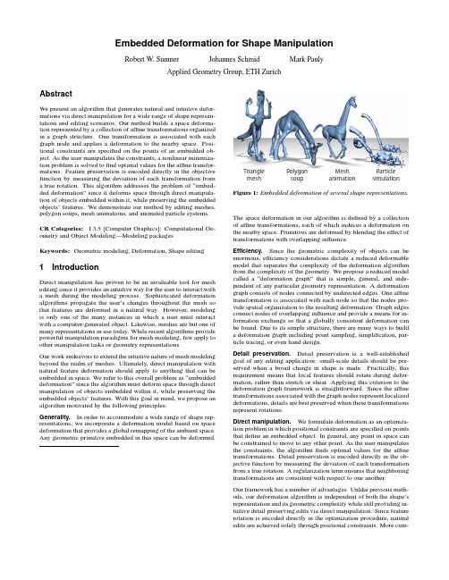
Embedded Deformation for Shape ManipulationRobert W.Sumner Johannes Schmid Mark PaulyApplied Geometry Group,ETH ZurichAbstractWe present an algorithm that generates natural and intuitive defor-mations via direct manipulation for a wide range of shape represen-tations and editing scenarios.Our method builds a space deforma-tion represented by a collection of afﬁne transformations organizedin a graph structure.One transformation is associated with eachgraph node and applies a deformation to the nearby space.Posi-tional constraints are speciﬁed on the points of an embedded ob-ject.As the user manipulates the constraints,a nonlinear minimiza-tion problem is solved toﬁnd optimal values for the afﬁne transfor-mations.Feature preservation is encoded directly in the objective function by measuring the deviation of each transformation from a true rotation.This algorithm addresses the problem of“embed-ded deformation”since it deforms space through direct manipula-tion of objects embedded within it,while preserving the embedded objects’features.We demonstrate our method by editing meshes, polygon soups,mesh animations,and animated particle systems.CR Categories:I.3.5[Computer Graphics]:Computational Ge-ometry and Object Modeling—Modeling packagesKeywords:Geometric modeling,Deformation,Shape editing1IntroductionDirect manipulation has proven to be an invaluable tool for mesh editing since it provides an intuitive way for the user to interact with a mesh during the modeling process.Sophisticated deformation algorithms propagate the user’s changes throughout the mesh so that features are deformed in a natural way.However,modeling is only one of the many instances in which a user must interact with a computer-generated object.Likewise,meshes are but one of many representations in use today.While recent algorithms provide powerful manipulation paradigms for mesh modeling,few apply to other manipulation tasks or geometry representations.Our work endeavors to extend the intuitive nature of mesh modeling beyond the realm of meshes.Ultimately,direct manipulation with natural feature deformation should apply to anything that can be embedded in space.We refer to this overall problem as“embedded deformation”since the algorithm must deform space through direct manipulation of objects embedded within it,while preserving the embedded objects’features.With this goal in mind,we propose an algorithm motivated by the following principles:Generality.In order to accommodate a wide range of shape rep-resentations,we incorporate a deformation model based on space deformation that provides a global remapping of the ambient space. Any geometric primitive embedded in this space can be deformed.PolygonsoupMeshanimationTrianglemeshParticlesimulation Figure1:Embedded deformation of several shape representations.The space deformation in our algorithm is deﬁned by a collection of afﬁne transformations,each of which induces a deformation on the nearby space.Primitives are deformed by blending the effect of transformations with overlapping inﬂuence.Efﬁciency.Since the geometric complexity of objects can be enormous,efﬁciency considerations dictate a reduced deformable model that separates the complexity of the deformation algorithm from the complexity of the geometry.We propose a reduced model called a“deformation graph”that is simple,general,and inde-pendent of any particular geometry representation.A deformation graph consists of nodes connected by undirected edges.One afﬁne transformation is associated with each node so that the nodes pro-vide spatial organization to the resulting deformation.Graph edges connect nodes of overlapping inﬂuence and provide a means for in-formation exchange so that a globally consistent deformation can be found.Due to its simple structure,there are many ways to build a deformation graph including point sampling,simpliﬁcation,par-ticle tracing,or even hand design.Detail preservation.Detail preservation is a well-established goal of any editing application:small-scale details should be pre-served when a broad change in shape is made.Practically,this requirement means that local features should rotate during defor-mation,rather than stretch or shear.Applying this criterion to the deformation graph framework is straightforward.Since the afﬁne transformations associated with the graph nodes represent localized deformations,details are best preserved when these transformations represent rotations.Direct manipulation.We formulate deformation as an optimiza-tion problem in which positional constraints are speciﬁed on points that deﬁne an embedded object.In general,any point in space can be constrained to move to any other point.As the user manipulates the constraints,the algorithmﬁnds optimal values for the afﬁne transformations.Detail preservation is encoded directly in the ob-jective function by measuring the deviation of each transformation from a true rotation.A regularization term ensures that neighboring transformations are consistent with respect to one another.Our framework has a number of advantages.Unlike previous meth-ods,our deformation algorithm is independent of both the shape’s representation and its geometric complexity while still providing in-tuitive detail preserving edits via direct manipulation.Since feature rotation is encoded directly in the optimization procedure,natural edits are achieved solely through positional constraints.More cum-bersome frame transformations are not required.The simplicity and ﬂexibility of the deformation graph make it easy to construct,since a rough distribution of nodes in the region that the user wishes to modify is sufﬁcient.Although the optimization is nonlinear,com-plex edits can be achieved with only a few hundred nodes.Thus, the number of unknowns is small compared to the geometric com-plexity of the embedded object.With our efﬁcient numerical im-plementation,even very detailed shapes can be edited interactively. Our primary contribution is a novel deformation representation and optimization procedure that unites the proven paradigms of direct manipulation and detail preservation with theﬂexibility of space deformations.We highlight the conceptual challenge of embedded deformation and provide a solution that expands intuitive editing to situations where it was previously lacking.Our method accom-modates traditional meshes with multiple connected components, polygon soups,point-based models with no connectivity informa-tion,and mesh animations.Our system also allows the user to in-teractively sculpt the result of a simulated particle system,easily creating effects that would be cumbersome and costly to achieve by tweaking simulation parameters(Figure1).2BackgroundEarly work in shape modeling focuses on space deformations[Barr 1984]that provide a global remapping of space.Free-form defor-mation(FFD)[Sederberg and Parry1988]parameterizes a space deformation with a3D lattice and provides an efﬁcient way to apply coarse deformations to complex shapes.However,achieving aﬁne-scale deformation may require a detailed,hand-designed control lattice[Coquillart1990;MacCracken and Joy1996]and an inordi-nate amount of user manipulation.Although more intuitive control can be provided through direct manipulation[Hsu et al.1992],the user is still restricted by the expressibility of the FFD algorithm. With their“Wires”concept,Singh and Fiume[1998]present aﬂex-ible and effective space deformation algorithm motivated by arma-tures used in traditional sculpting.A collection of space curves tracks deformable features of an object,providing a coarse approx-imation to the shape and a means to deform it.Singh and Kokke-vis[2000]generalize this concept to a polygon-based deformer.In both cases,the user interacts solely with the proxy curves or poly-gons rather than directly with the object being deformed.Rotations, scales,and translations are inferred from the user interaction and applied to the object.These methods give the user powerful tools to design deformations and add detail to a shape.However,they are not well suited to modify shapes that already are highly detailed since the user must design armature curves or control polygons that conform to details at the proper scale in order for the deformation heuristics to generate acceptable results.Due to the widespread availability of very detailed scanned meshes, recent research focuses on high-quality mesh editing through intu-itive user interfaces.Detail preservation is a central goal of such algorithms.Multiresolution methods achieve detail-preserving ed-its at varying scales by generating a hierarchy of simpliﬁed meshes together with corresponding detail coefﬁcients[Kobbelt et al.1998; Botsch and Kobbelt2004].While models with large geometric de-tails may lead to local self-intersections or other artifacts[Botsch et al.2006b],the modeling metaphor presented by Kobbelt and col-leagues[1998]in which a region-of-interest and handle region are deﬁned directly on the mesh is especially notable as it has been applied in nearly every subsequent mesh editing paper. Algorithms based on differential representations extract local shape properties,such as curvature,scale,and orientation.By represent-ing a mesh in terms of these values,editing can be phrased as an energy minimization problem that strives to preserve them[Sorkine 2005].Methods that perform only linear system solves require heuristics or other special treatment of feature rotation,since natu-ral shape deformation is inherently nonlinear[Botsch and Sorkine 2007].V olumetric methods(e.g.,[Zhou et al.2005;Shi et al.2006]) build a dissection of the interior and nearby exterior space for better volume preservation,while subspace methods[Huang et al.2006] build a subspace structure for increased efﬁciency and stability. Nonlinear methods(e.g.,[Sheffer and Kraevoy2004;Huang et al. 2006;Botsch et al.2006a])yield the highest quality edits,although at higher computational costs.These algorithms provide powerful tools for detail-preserving mesh editing.However,these and other mesh editing techniques do not meet the goals of embedded deformation since the deformation al-gorithm is intimately tied to the shape representation.For example, in the method presented by Huang and colleagues[2006],detail preservation is expressed as a mesh-based Laplacian energy that is computed in terms of vertices and their one-ring neighbors.The work of Shi and colleagues[2006]and Zhou and colleagues[2005] both use a Laplacian energy term based on a mesh representation. The prism-based technique of Botsch and colleagues[2006a]uses a deformation energy deﬁned through a coupling of prisms along mesh edges and requires a mesh representation with consistent connectivity.These techniques do not apply to non-meshes,such as point-based representations,particle systems,or polygon soups where no connectivity structure can be assumed.With our method,we adapt the intuitive click-and-drag modeling metaphor used in mesh editing to the context of space deforma-tions.Like Wires[Singh and Fiume1998]and its polygon-based extension[Singh and Kokkevis2000],our method is not tied to one particular representation and can be applied to any primitive de-ﬁned by points in3D.However,unlike Wires or other space defor-mation algorithms that do not explicitly preserve details[Hsu et al. 1992;Botsch and Kobbelt2005],we successfully formulate detail preservation within the space deformation framework.The com-plexity of our deformation graph is independent of the complexity of the shape being edited so that our technique can handle detailed shapes interactively.The graph need not be a volumetric dissec-tion and is simpler to construct than the volumetric or subspace structures used by previous methods.The optimization problem is nonlinear and exhibits comparable quality to nonlinear mesh-based algorithms with less computational cost.Thus,our algorithm com-bines theﬂexibility of space deformations to deform any primitive independent of its geometric complexity with a simple and intuitive click-and-drag interface and high-quality detail preservation.3Deformation GraphThe primary challenge of embedded deformation is toﬁnd a defor-mation model that is general enough to apply to any object embed-ded in space yet still provides intuitive direct manipulation,natural feature preservation,and efﬁciency.We meet these goals with a novel reduced deformable model called a“deformation graph”that can express complex deformations of a variety of shape representa-tions.In this model,a space deformation is deﬁned by a collection of afﬁne transformations.One transformation is associated with each node of a graph embedded in R3,so that the graph provides spatial organization to the deformation.Each afﬁne transformation induces a localized deformation on the nearby space.Undirected edges connect nodes of overlapping inﬂuence to indicate local de-pendencies.The node positions are given by g j∈R3,j∈1...m, and the set N(j)consists of all nodes that share an edge with node j. The afﬁne transformation for node j is speciﬁed by a3×3matrix R j and a3×1translation vector t j.The inﬂuence of the transfor-mation is centered at the node’s position so that it maps any point p in R3to the position˜p according to˜p=R j(p−g j)+g j+t j.(1) A deformed version of the graph itself is computed by applying each afﬁne transformation to its corresponding node.Since g j−g jis the zero vector,the deformed position˜g j of node j is simply equal to g j+t j.More interestingly,the deformation graph can be used to deform any geometric model deﬁned by vertices in R3.Since transfer-ring the deformation to an embedded shape requires computation proportional to the shape’s complexity,efﬁciency is of paramount importance.Consequentially,we employ an algorithm similar to the widely used and highly efﬁcient skeleton-subspace deformation from character animation.The inﬂuence of individual graph nodes is smoothly blended so that the deformed position˜v i of each shape vertex v i,i∈1...n,is a weighted sum of its position after applica-tion of the deformation graph afﬁne transformations:˜v i=m∑j=1w j(v i)R j(v i−g j)+g j+t j.(2)While linear blending may result in some artifacts for extremely coarse graphs,they are negligible for moderately dense ones like those shown in our examples.This result is not surprising,since only a few extra joint transformations are needed to greatly reduce artifacts exhibited by skeleton-subspace deformation[Weber2000; Mohr and Gleicher2003].In our case,the nodes are evenly dis-tributed over the entire shape so that the blended transformations are very similar to one another.Normals are transformed similarly,according to the weighted sum of each normal transformed by the inverse transpose of the node transformations,and then renormalized:˜n i=m∑j=1w j(v i)R−1jn i.(3)The weights w j(v i),j∈1...m,are spatially varying and thus de-pend on the vertex position.Due to the graph structure,transforma-tions that are close to one another will be the most similar.Thus,for consistency and efﬁciency,we limit the inﬂuence of the deforma-tion graph on a particular vertex to the k-nearest nodes.The weights for each vertex are precomputed according tow j(v i)=(1− v i−g j /d max)2(4)and then normalized to sum to one.Here,d max is the distance to the k+1-nearest node.We use k=4for all examples,except the experiment in Figure5(d),where k=8.The layout of the deformation graph nodes should roughly conform to the shape of the model being edited.In our experiments,a uni-form sampling of the model surface produces the best results.Such a sampling is easily accomplished by distributing points densely over the surface,and repeatedly removing all points within a given radius of a randomly chosen one until a desired sampling density is reached.For meshes,simpliﬁcation algorithms also produce good results when the triangle aspect ratio is restricted to avoid long andskinnytriangles.For particle simulations,a simple and efﬁcientconstruction of the node layout can be achieved by sampling parti-cle paths through time.The number of graph nodes determines the expressibility of the deformation graph.Coarse editscan be made with a small number of nodes,while highly detailed ones require denser sampling.Weﬁnd that full body pose changes are effec-tively accomplished with200to300nodes.Graph edges connect nodes of overlapping inﬂuence and are used to enforce consistency in the overall deformation.Once the node po-sitions are determined,the connectivity is computed automatically by creating an edge between any two nodes that inﬂuence the same vertex.Thus,the graph structure depends on how it is evaluated.01234E conE con+E regE con+E reg+E rotR2(g3−g2)+g2+tg2)+g2+t2g2+t2Figure2:A simple deformation graph shows the effect of the three terms of the objective function.The quadrilaterals at each graph node illustrate the deformation induced by the corresponding afﬁne transformation.Without the rotational term,unnatural shearing can occur,as shown in the bottom right.The transformation for node g2is applied to neighboring nodes g1and g3,yielding the predicted positions shown on the bottom left as gray circles.The regularization term minimizes the squared distance between these predicted positions and their actual positions˜g1and˜g3.4OptimizationOnce the deformation graph has been speciﬁed,the user manipu-lates an embedded primitive by selecting vertices and moving them around.The vertices serve as positional constraints for an opti-mization problem in which the afﬁne transformations of the de-formation graph comprise the unknown variables.The objective function encodes detail preservation directly by specifying that the afﬁne transformations should be rotations.Consequently,local fea-tures deform as rigidly as possible.A second energy term serves as a regularizer for the deformation by indicating that the afﬁne trans-formations of adjacent graph nodes should agree with one another. Rotation.In order for a3×3matrix R to represent a rotation in SO(3),it must satisfy six conditions:each of its three columns must be unit length,and all columns must be orthogonal to one an-other[Grassia1998].The squared deviation from these conditions is given by the function Rot(R):Rot(R)=(c1·c2)2+(c1·c3)2+(c2·c3)2+(c1·c1−1)2+(c2·c2−1)2+(c3·c3−1)2(5)where c1,c2,and c3are the3×1column vectors of R.This func-tion is nonlinear in the matrix entries.The term E rot sums the rota-tion error over all transformations of the deformation graph:E rot=m∑j=1Rot(R j).(6)Regularization.Conceptually,each of the afﬁne transformations represents a localized deformation centered at a graph node.Since nearby transformations have overlapping inﬂuence,we must ensure that the computed transformations are consistent with respect to one another.We add a regularization term to the optimization inferred from the graph structure.If nodes j and k are neighbors,they affect a common subset of the embedded shape.The position of node kpredicted by node j’s afﬁne transformation should match the actual position given by applying node k’s transformation to itself(Fig-ure2).The regularization error E reg sums the squared distances between each node’s transformation applied to its neighbors and the actual transformed neighbor positions:E reg=m∑j=1∑k∈N(j)αjkR j(g k−g j)+g j+t j−(g k+t k)22.(7)The weightαjk should be proportional to the degree to which the inﬂuence of nodes j and k overlap.However,the exact amount of overlap is ill deﬁned for many shape representations,such as point-based models and animated particle systems.In order to meet our goal of generality,we useαjk=1.0for all examples.We notice no artifacts compared to experiments using other weighting schemes. This regularization equation bears some resemblance to the defor-mation smoothness energy term used by previous work on template deformation[Allen et al.2003;Sumner and Popovi´c2004;Pauly et al.2005].However,the transformed vertex positions are com-pared,rather than the transformations themselves,and the transfor-mations are relative to the node positions,rather than to the global coordinate system.Constraints.The user controls the optimization through direct manipulation of the embedded shape and need not be aware of the underlying deformation graph.To facilitate editing,our algorithm supports two types of constraints:handle constraints,where a col-lection of model vertices are selected and become handles that are manipulated by the user,andﬁxed constraints,where a collection of model vertices are selected and guaranteed to beﬁxed in place. Handle constraints comprise the interface with which the user in-teracts with an embedded object.These positional constraints are speciﬁed by selecting and moving model vertices.They inﬂuence the optimization since the deformed vertex positions are a function of the graph’s afﬁne transformations.We enforce these constraints using a penalty formulation according to the term E con which is included in the objective function:E con=p∑l=1˜v index(l)−q l22.(8)Vertex˜v index(l)is deformed by the deformation graph according to Eq.2.The vector q l is the user-speciﬁed position of constraint l, and index(l)is the index of the constrained vertex.Fixed constraints are speciﬁed through the same selection mech-anism as handle constraints.However,they are implemented by treating all node transformations that inﬂuence the selected vertices as constants,rather than free variables,and removing them from the optimization procedure.Their primary function is to allow the user to deﬁne the portion of the mesh which is to be edited.Fixed con-straints incur no computational overhead.Conversely,they speed up the computation by reducing the number of unknowns.Thus, the user can make aﬁne-scale edit by using a dense deformation graph and marking all parts of the embedded object not in the edit region asﬁxed.Numerics.Our shape editing framework solves the following op-timization problem:minR1,t1...R m,t mw rot E rot+w reg E reg+w con E con.subject to R q=I,t q=0,∀q∈ﬁxed ids(9)We use the weights w rot=1,w reg=10,and w con=100for all ex-amples.Eq.9is nonlinear in terms of the12m unknowns that deﬁne the afﬁne transformations.Fixed constraints are handled trivially by treating the constrained variables as constants,leaving12m−12q free variables if there are qﬁxed transformations.We implement the iterative Gauss-Newton algorithm to solve the resulting uncon-strained nonlinear least-squares problem[Madsen et al.2004]. The Gauss-Newton algorithm linearizes the nonlinear problem with Taylor expansion about x:f(x+δ)=f(x)+Jδ(10) The vector f(x)stacks the equations that deﬁne the objective func-tion so that f(x) f(x)=F(x)=w rot E rot+w reg E reg+w con E con,the vector x stacks the entries in the afﬁne transformations,and J is the Jacobian matrix of f(x).Each Gauss-Newton iteration solves a lin-earized problem to improve x k,the current estimate of the unknown transformations:δk=argminδf(x k)+Jδ 22x k+1=x k+δk.(11)The process repeats until convergence,which we detect by moni-toring the change in the objective function F k=F(x k),the gradient of the objective function,and the magnitude of the update vectorδk [Gill et al.1989]:|F k−F k−1|<ε(1+F k)∇F k ∞<3√ε(1+F k)(12)δk ∞<2√ε(1+ δk ∞).In our experiments,the optimization converges after about six iter-ations withε=1.0×10−6.In each iteration,we solve the resulting normal equations by Cholesky factorization.Although the linear system J J is very sparse,it depends on x and thus changes at each iteration.There-fore,the full factorization cannot be reused.However,the non-zero structure remains unchanged so that aﬁll-reducing permutation of the matrix and symbolic factorization based only on its non-zero structure can be precomputed and reused[Toledo2003].These steps,together with careful implementation of the routines to build J and J J,result in a very efﬁcient solver.As shown in Table1, each iteration requires about20ms for the presented examples.5ResultsWe have implemented the deformation graph optimization both as an interactive editing application as well as an ofﬂine system for applying scripted constraints to animated data.Live edits with the interactive application are demonstrated in the conference video, and key results are highlighted in this section.Detail preservation.Figure3demonstrates that our algorithm preserves features of the embedded shape.A bumpy plane is mod-iﬁed byﬁxing vertices on the left in place and translating those on the right upward.Although this edit is purely translational,the optimizationﬁnds node transformations that are as close as possi-ble to true rotations while meeting the vertex constraints and main-taining consistency.As a result,the bumps on the plane deform in a natural fashion without shearing artifacts.These results are comparable to the nonlinear prism-based approach of Botsch and colleagues[2006a].However,our algorithm uses a deformation graph of only299nodes,whereas Botsch’s method performs the optimization on the full40,401vertex model and requires a con-sistent meshing of the surface.Figure3also demonstrates that our method preserves details better than the radial-basis function(RBF) approach of Botsch and Kobbelt[2005],where feature rotation is not considered.Figure4demonstrates detail preservation on a more complex exam-ple.With a graph of only222nodes,our approach achieves a defor-mation comparable in quality to the subspace method of Huang andOriginal surface 40,401 vertices Deformation graph299 nodesDeformeddeformation graphDeformed surface PriMo approach of[Botsch et al. 2006]RBF approach of[Botsch & Kobbelt 2005] Figure3:When used to deform a bumpy plane,our method accurately preserves features without shearing or stretching artifacts.The quality of our results is comparable to the“PriMo”approach of Botsch and colleagues[2006a]and superior to the radial-basis function method of Botsch and Kobbelt [2005].Original graphsDeformed graphsDeformed 222 nodes Deformed425 nodesDeformed1,048 nodesOriginalFigure4:We perform an edit similar to the one shown in Figure9 of the work of Huang and colleagues[2006].With a graph of only 222nodes,our results are of comparable quality to Huang’s sub-space gradient domain method.Performing the identical edit with more complex graphs does not yield a signiﬁcant change in quality.colleagues[2006]in which the Laplacian energy is enforced on the full mesh.Higher resolution graphs do not signiﬁcantly improve quality.Performing the same editing task with graphs of425and 1,048nodes yields nearly identical results.Of course,if the graph becomes too sparse to match the complexity of the deformation,ar-tifacts will occur,as can be expected with any reduced deformable model.Likewise,in the highly regular setting shown in Figure5, minor artifacts appear as a slight striped pattern.If additional nodes are used for interpolation or a less regular graph(Figure3),no arti-facts are noticeable.Intuitive editing.Figures6and7demonstrate the intuitive edit-ing framework enabled by our system.High-quality edits are achieved by placing only a handful of single-vertex handle con-straints on the shape.Figure6shows detail-preserving edits on a mesh consisting of85,792vertices.The raptor is deformed by dis-placing positional constraints only,without the need to explicitly specify frame rotations.Fine-scale details such as the teeth and wrinkles are preserved.Furthermore,when the head or body is ma-nipulated and the arms are left unconstrained,the arms rotate in a natural way to follow the body movement.Thus,features are pre-served at a wide range of scales.In this example,a full body pose is sculpted using a graph of226nodes.The tail is lifted,arms crossed, left leg moved forward,and head rotated to look backward.Then, localized changes to the head are made with a more detailed graph of840nodes.However,ﬁxed constraints speciﬁed by selecting the(a)(b)(c)(d)Figure5:A highly regular deformation graph with200nodes, shown in(a),is used to create the deformation in(b).In this struc-tured setting,minor artifacts are visible on the13,024vertex plane, shown in(c),as a slight striped pattern when k=4graph nodes are used for transforming the mesh vertices.These artifacts disappear in(d)when k=8nodes are used and are not present with less struc-tured graphs(Figure3).raptor’s body(green)leave only138active nodes for the head edit so that the system remains interactive.Figure7shows interactive edits on a scanned toy giraffe.The model consists of a set of un-merged range scans that contain many holes and outliers,with a total of79,226vertices in180separate con-nected components.The deformation graph consisting of221nodes is built automatically via uniform sampling,allowing the user to directly edit the shape without time-consuming pre-processing to obtain a consistent mesh representation.Mesh animations.In addition to static geometry,our approach also supports effective editing of dynamic shapes.The mesh anima-tion of Figure8is modiﬁed to lengthen the horse’s legs and neck, and turn its head.The deformation graph,constructed with mesh simpliﬁcation,is advected passively with the animated mesh.Since the graph nodes are chosen to coincide with mesh vertices,no addi-tional computation is required for the node positions to track the an-imation.The user can script edits by setting keyframes on a single pose.Translational offsets are computed from this keyframe data and applied frame-by-frame to the animation sequence with our of-ﬂine application.The graph structure and weighting remainsﬁxed throughout the animation.The output mesh animation incorpo-rates the user’s edits while preserving geometric details,such as the horse’s facial features,as well as high-frequency motion,such as the head bobbing.No multiresolution hierarchy or signal process-ing is needed,unlike the method of Kircher and Garland[2006]. Although we do not address temporal coherence directly,we no-ticed no coherence artifacts in our experiments.Particle simulations.The particle simulation shown in Figure9 is another example of a dynamic shape that can be edited with the deformation graph framework.Our system allows small-scale cor-rections that would be tedious to achieve by tweaking simulation parameters,as well as more drastic modiﬁcations that go beyond the capabilities of a pure simulation.In this example,particle posi-tions are precomputed with aﬂuid simulation.A linear deformation graph is built by sampling the path that a single particle travels over。

一种基于小波邻域的半软阈值去噪算法

一种基于小波邻域的半软阈值去噪算法
赵新中;陶永耀;贺佩;石敏
【期刊名称】《国外电子测量技术》
【年(卷),期】2016(0)4
【摘要】针对小波硬阈值去噪函数的不连续和软阈值去噪函数的恒定偏差导致图像边缘模糊的缺点,本文提出了一种新的半软阈值函数。

该方法通过区分图像的强弱边缘分别进行处理,并在弱边缘小波系数的估计中采取基于贝叶斯估计的方法且考虑了邻域小波系数的大小。

仿真结果表明,与原有的小波阈值去噪算法和普通的阈值去噪算法相比,该算法在峰值信噪比(PSNR)、边缘保持指数(EPI)和视觉效果上都有明显的提高。

该方法能够很好地保护图像边缘信息,达到很好的去噪效果。

【总页数】4页(P42-45)
【关键词】弱边缘;邻域小波系数;半软阈值函数;边缘保持指数
【作者】赵新中;陶永耀;贺佩;石敏
【作者单位】炬芯(珠海)科技有限公司;暨南大学信息科学技术学院
【正文语种】中文
【中图分类】TN911.73
【相关文献】
1.一种超限像素平滑和小波软阈值图像去噪算法 [J], 杨永波;陈君芸
2.基于小波邻域阈值分类的电能质量信号去噪算法 [J], 张明;李开成;胡益胜
3.基于邻域阈值分类的小波域图像去噪算法 [J], 侯建华;熊承义;田金文;柳健
4.一种新的小波半软阈值图像去噪方法 [J], 李秋妮;晁爱农;史德琴;孔星炜
5.基于混沌搜索的改进小波半软阈值去噪 [J], 张沫;席剑辉
因版权原因，仅展示原文概要，查看原文内容请购买。

IND560 weighing terminal和Fill-560应用软件商品说明书

2Industrial Weighing and MeasuringDairy & CheeseNewsIncrease productivitywith efficient filling processesThe new IND560 weighing terminal enables you to boost speed and precision during the filling process. Choose from a wide range of scales and weigh modules to connect to the terminal.The versatile IND560 excels in control-ling filling and dosing applications, delivering best-in-class performance for fast and precise results in manual, semi-automatic or fully automatic operations. For more advanced filling, the Fill-560 application software adds additional sequences and component inputs. Without complex and costly programming you can quickly con-figure standard filling sequences, or create custom filling and blending applications for up to four compo-nents, that prompt operators for action and reduce errors.Ergonomic design Reducing operator errors is achieved through the large graphic display which provides visual signals.SmartTrac ™, the METTLER TOLEDO graphical display mode for manual operations, which clearly indicate sta-tus of the current weight in relation to the target value, helps operators to reach the fill target faster and more accurately.Connectivity and reliabilityMultiple connectivity options are offered to integrate applications into your con-trol system, e.g. Allen-Bradley ® RIO, Profibus ®DP or DeviceNet ™. Even in difficult vibrating environments, the TraxDSP ™ filtering system ensures fast and precise weighing results. High reli-ability and increased uptime are met through predictive maintenance with TraxEMT ™ Embedded MaintenanceTechnician.METTLER TOLEDO Dairy & Cheese News 22Speed up manual operations with flexible checkweighingB e n c h & F l o o r S c a l e sHygienic design, fast display readouts and the cutting-edge color backlight of the new BBA4x9 check scales and IND4x9 terminals set the standard for more efficient manual weigh-ing processes.Flexibility through customizationFor optimal static checkweighing the software modules ‘check’ and‘check+’ are the right solutions. They allow customization of the BBA4x9 and the IND4x9 for individual activi-ties and needs, e.g. manual portion-ing or over/under control. Flexibility is increased with the optional battery which permits mobility. Hygienic design Easy-to-clean equipment is vital in food production environments. Both the BBA4x9 scale and the IND4x9 ter-minal are designed after the EHEDGand NSF guidelines for use in hygi-enically sensitive areas.Even the back side of the scale stand has a smooth and closed surfacewhich protects from dirt and allowstrouble-free cleaning.Fast and preciseThe colorWeight ® display with a colored backlight gives fast, clear indication when the weight is with-in, below or above the tolerance.The color of the backlight can be chosen (any mixture of red, greenand blue) as well as the condition itrefers to (e.g. below tolerance). The ergonomic design enables operators to work more efficiently due to less exhaustion.Short stability time, typically between 0.5s and 0.8s, ensures high through-put and increased productivity.PublisherMettler-Toledo GmbH IndustrialSonnenbergstrasse 72CH-8603 Schwerzenbach SwitzerlandProductionMarCom IndustrialCH-8603 Schwerzenbach Switzerland MTSI 44099754Subject to technical changes © 06/2006 Mettler-Toledo GmbH Printed in SwitzerlandYellow – weight above toleranceGreen – weight within toleranceRed – weight below toleranceYour benefits• Fast and precise results and operations • Higher profitability• Ergonomic design, simple to operate • Mobility up to 13h due to optional batteryFast facts BBA4x9 and IND4x9• 6kgx1g, 15kgx2g, 30kgx5g (2x3000d), for higher capacity scales: IND4x9 terminal • Weights and measures approved versions 2x3000e • Functions: simple weighing, static checkweighing, dispensing • Color backlight, bar graph • Tolerances in weight or %• 99 Memory locations • Optional WLAN, battery• Meets the IP69k protection standardsagainst high-pressure and steam cleaning • Complete stainless steel construction Immediate checkweighing resultswith color Weight®EHEDGThe colored backlight of the LC display provides easy-to- recognize indication whether the weight is within the tolerancelimits or not.WLANMETTLER TOLEDO Dairy & Cheese News 23HACCP programs, GMP (Good Manufacturing Practice), pathogen monitoring and good cleaning practices are essential for effective food safety plans. Our scales are constructed for compliance with the latest hygienic design guidelines.Hygienic design to improve food safetyMETTLER TOLEDO supports you in complying with the latest food safety standards like BRC, IFS or ISO 22000 by offering solutions which are:• Compliant with EHEDG (European Hygienic Engineering & Design Group) and NSF (National Sanitation Foundation) guidelines • Full V2A stainless steel construc-tions, optional V4A load plates • Smooth surface (ra < 0.8μm)• Easy-to-clean construction, no exposed holes • Radius of inside corners > 3mm• Ingress protection rating up to IP69k• Hermetically sealed loadcellsYour benefits• Reduce biological and chemical contamination risks • Fast and thorough cleaning procedures • Fulfillment of hygiene regulations • Long equipment life thanks to rugged designGuaranteed serviceKeep your business runningAvoid unnecessary downtime with our wide range of service packages.With a range of innovative service solutions offering regulatory compli-ance, equipment calibration, train-ing, routine service and breakdown assistance, you can profit from sus-tained uptime, together with ongoing performance verification and long life of equipment. There is a range of contract options designed to comple-ment your existing quality systems. Each one offers its own unique set of benefits depending on the equipment and its application.4/serviceFast facts PUA579 low profile scale • 300kgx0.05kg – 1500kgx0.2kg • Open design• Lifting device for easy cleaning • EHEDG conform(300 and 600kg models -CS/-FL)• Free size scale dimensions • Approach rampsExample:PUA579 first EHEDG conform floor scaleEHEDGW e i g h P r i c e L a b e l i n gChallenges faced in the packaging area are:• Responding quickly to retailer demands while improving margins • Improving pack presentation • Minimizing downtime and product giveawaysWith a complete offering of cutting-edge weighing technology, high-per-formance printing, and smart soft-ware solutions, we can help you tackle your labeling challenges whether they are very simple or highly demanding. Intuitive human-machine interfaceTouch-screen operator displays withgraphical icons guide the operator intuitively and reduce nearly every operation to just one or two key-strokes. This interface allows reduced operator training as well as increased operating efficiency.Advanced ergonomics and sani-tary designOur weigh-price labelers are made out of stainless steel for extensive pro-tection against food contamination. Careful attention to hygienic design requirements, with no dead spots and few horizontal parts, ensure that the labelers are easy to clean.Modular designOur product offering includes both manual and automatic weigh-price labelers constructed of flexible “build-ing blocks.” Different combinations and configurations can meet specific budget and operational requirements. METTLER TOLEDO will help you toselect the right:• Scale performance • Display technology • Memory capacity • IT connections • Degree of automation• Integration kitsA large range of options and peripher-als give flexibility for meeting unique requirements e.g. wireless network, hard disks, external keyboards, bar code scanners, RFID transponder, dynamic checkweighing, or metal detection.Weigh-price-labeling Ergonomic, modular, fastEtica 2300 standard manual labelerFor individual weight labeling of various products, high- speed weighing, smart printing and fast product changes are essential. METTLER TOLEDO offers static and automated solutions for both manual and high-speed prepack applica-tions. Choose from our Etica and PAS product range.METTLER TOLEDO Dairy & Cheese News 24Etica 2400i combination with automatic stretch wrappersEtica 2430G multi-conveyer weigh-price labeler rangeEfficient label applicatorsThe unique Etica label applicator (Etica G series) does not require an air compressor, allowing savings on initial equipment expense and ongo-ing maintenance costs. Labels are gently applied in any pre-memorized orientation.PAS systems provide motorized height adjustment and places the label in any corner of the package. Users will have a new degree of freedom in planning their case display layouts to maximize both product presentation and consumer impact.Smart label design tools Retailers want labels to carry clear, correct information, in accordance with their traceability and style requirements. Our solutions are equipped with labeldesign software tools which facili-tate the design of labels customizedfor retailers demands. A touch-screenallows the user to create specific labels– even with scanned elements such aslogos and graphics, pre-programmedlabel templates, or RFID.Versatile integration capabilitiesThe engineers at METTLER TOLEDOworked closely with Europe’s leadingautomatic stretch wrapper suppliersto design performance-enhancingand cost-effective weigh-wrap-labelsystem solutions. Achieving a smallsystem footprint means the systemsrequire only slightly more floor spacethan the wrapper alone.The PAS and Etica weigh-price label-ers can be integrated via TCP/IP ina METTLER TOLEDO scale network,in host computer systems and goodsmanagement systems.Etica weigh-price-labeling systems• Static and automatic weigh-price-labeling up to 55 pieces/min.• Operator displays:– 5.7” color back-lighted LCD (Etica 2300 series)– 10.4” high resolution touch screen (Etica 4400 series)• 3 inch graphic thermal printer (125 to 250mm/sec) withfully programmable label format (max. size 80x200mm)• Data memory:– 64 to 256 Mb RAM– 128 Mb to 10 Gb mass storage– Unlimited number of logo graphics and label descriptions• Interfaces:– 1 serial RS232 interface– Optional second RS232 + RS485 + Centronics port– Ethernet network communication interface(10baseT), TCP/IP, 2 USB ports (1)– Optional: hand-held bar code scanner for automatictraceability data processingGarvens PAS 3008/3012 price labelersEtica 4400METTLER TOLEDO Dairy & Cheese News 2FlexMount ® weigh moduleFast, reproducible and reliable batch-ing and filling are key success factors for your production process. Various factors can affect precision: foam can compromise optical/radar sensors, and solids do not distribute evenly in a tank or silo. Our weighing techno-logy is not affected by these condi-tions and provides direct, accurate and repeatable measurement of mass without media contact. In addition our range of terminals and transmit-ters/sensors enable easy connectivity to your control systems.Key customer benefits• Increased precision and consistencyof your material transfer processes• Faster batching process throughsupreme TraxDSP ™ noise and vibration filtering • Minimal maintenance cost Fast facts terminals/transmitters: PTPN and IND130• Exclusive TraxDSP ™ vibration rejection and superior noise filter-ing system • Easy data integration through a variety of interfaces, including Serial, Allen-Bradley ® RIO, Modbus Plus ®, Profibus ® and DeviceNET • IP65 stainless harsh versionsProcess terminal PTPN• Local display for weight indication and calibration checks • Panel-mount or stainless steel desk enclosureIND130 smart weight transmitter• Direct connectivity where no local display is required • Quick setup and run via PC tool • CalFREE ™ offers fast and easy cali-bration without test weights • DIN rail mounting versionPLCIND1306Tank and silo weighing solutions master your batching processesT a n k & S i l o W e i g h i n g S o l u t i o n sBoost your productivity and process uptime with reliable weighing equipment – improved batching speed and precision, maximum uptime at low maintenance cost.TraxDSP ™ ensures accurate results evenin difficult environments with vibrationPTPN process terminalMETTLER TOLEDO Dairy & Cheese News 27Quality data under control?We have the right solutionConsistently improving the quality of your products requires the ability of efficiently controlling product and package quality parameters in a fast-changing and highly competi-tive environment.Competition in the food industry –with high volumes but tight margins – causes demands for efficient quality assurance systems. Statistical Quality Control (SQC) systems for permanent online information and documenta-tion about your key quality para-meters convert into real cost savings.Our solutions for Statistical Quality Control (SQC) combine ease of opera-tion, quality data management and analysis functionality.• We offer mobile compact solutions with embedded SQC intelligence up to networked systems with an SQL database.• The systems are upgradeable and can be expanded and adapted to meet changing customer needs.• Simple and intuitive prompts guide the user through the sample proc-ess, reducing training costs as well as sampling errors.• Realtime analysis and alarms help to take immediate corrective measures and to save money by reducing overfilling.Throughout the manufacturing pro-cess, METTLER TOLEDO SQC solu-tions analyze your important product and package quality parameters andpresent them the way you want, help-ing to comply to legislation, to control and document your product qualityand your profitability.Metal detectionCheckweigher Sample check ® onlinequality data analysis/dairy-cheeseFor more informationMettler-Toledo GmbH CH-8606 Greifensee SwitzerlandTel. +41 44 944 22 11Fax +41 44 944 30 60Your METTLER TOLEDO contact:1. SevenGo ™ portable pH-meter2. In-line turbidity, pH and conductivity sensors3. DL22 Food and beverage analyzer4. Halogen moisture analyzersA wide range of solutions to improve processes1. Statistical Quality Control/Statistical Process Control2. Process weighing3. Predictive maintenance4. Methods of moisture content determinationShare our knowledgeLearn from our specialists – our knowledge and experience are at your disposal in print or online.Learn more about all of our solutions for the dairy and cheese industry at our website. You can find information on a wide range of topics to improve your processes, including case studies,application stories, return-on invest-ment calculators, plus all the product information you need to make aninformed decision.1 2 341423。

翻译Speeded-up Robust Features

Speeded-Up Robust Features (SURF)Herbert Bay, Andreas Ess, Tinne Tuytelaars, Luc Van Gool摘要这篇文章提出了一种尺度和旋转不变的检测子和描述子，称为SURF(Speeded-Up Robust Features)。

SURF在可重复性、鉴别性和鲁棒性方面都接近甚至超过了以往的方案，同时计算和比较的速度更快。

这依赖于使用了积分图进行图像卷积、使用现有的最好的检测子和描述子（特别是，基于Hessian矩阵方法的检测子，和基于分布的描述子）、以及简化这些算法到了极致。

这些最终实现了新的检测、描述和匹配过程的结合。

本文包含对检测子和描述子的详细阐述，之后探究了一些关键参数的作用。

作为结论，我们用两个目标相反的应用测试了SURF的性能：摄像头校准（图像配准的一个特列）和目标识别。

我们的实验验证了SURF在计算机视觉广泛领域的实用性。

1.引言在两个图片中找到相似场景或目标的像素点一致性，这是许多计算机视觉应用中的一项任务。

图像配准，摄像头校准，目标识别，图像检索只是其中的一部分。

寻找离散像素点一致性的任务可以分为三步。

第一，选出兴趣点并分别标注在图像上，例如拐角、斑块和T型连接处。

兴趣点检测子最有价值的特性是可重复性。

可重复性表明的是检测子在不同视觉条件下找到相同真实兴趣点的能力。

然后，用特征向量描述兴趣点的邻域。

这个描述子应该有鉴别性，同时对噪声、位移、几何和光照变换具有鲁棒性。

最后，在不同的图片之间匹配特征向量。

这种匹配基于向量间的马氏或者欧氏距离。

描述子的维度对于计算时间有直接影响，对于快速兴趣点匹配，较小的维度是较好的。

然而，较小的特征向量维度也使得鉴别度低于高维特征向量。

我们的目标是开发新的检测子和描述子，相对于现有方案来说，计算速度更快，同时又不牺牲性能。

为了达成这一目标，我们必须在二者之间达到一个平衡，在保持精确性的前提下简化检测方案，在保持足够鉴别度的前提下减少描述子的大小。

A Fast and Accurate Plane Detection Algorithm for Large Noisy Point Clouds Using Filtered Normals

A Fast and Accurate Plane Detection Algorithm for Large Noisy Point CloudsUsing Filtered Normals and Voxel GrowingJean-Emmanuel DeschaudFranc¸ois GouletteMines ParisTech,CAOR-Centre de Robotique,Math´e matiques et Syst`e mes60Boulevard Saint-Michel75272Paris Cedex06jean-emmanuel.deschaud@mines-paristech.fr francois.goulette@mines-paristech.frAbstractWith the improvement of3D scanners,we produce point clouds with more and more points often exceeding millions of points.Then we need a fast and accurate plane detection algorithm to reduce data size.In this article,we present a fast and accurate algorithm to detect planes in unorganized point clouds usingﬁltered normals and voxel growing.Our work is based on aﬁrst step in estimating better normals at the data points,even in the presence of noise.In a second step,we compute a score of local plane in each point.Then, we select the best local seed plane and in a third step start a fast and robust region growing by voxels we call voxel growing.We have evaluated and tested our algorithm on different kinds of point cloud and compared its performance to other algorithms.1.IntroductionWith the growing availability of3D scanners,we are now able to produce large datasets with millions of points.It is necessary to reduce data size,to decrease the noise and at same time to increase the quality of the model.It is in-teresting to model planar regions of these point clouds by planes.In fact,plane detection is generally aﬁrst step of segmentation but it can be used for many applications.It is useful in computer graphics to model the environnement with basic geometry.It is used for example in modeling to detect building facades before classiﬁcation.Robots do Si-multaneous Localization and Mapping(SLAM)by detect-ing planes of the environment.In our laboratory,we wanted to detect small and large building planes in point clouds of urban environments with millions of points for modeling. As mentioned in[6],the accuracy of the plane detection is important for after-steps of the modeling pipeline.We also want to be fast to be able to process point clouds with mil-lions of points.We present a novel algorithm based on re-gion growing with improvements in normal estimation and growing process.For our method,we are generic to work on different kinds of data like point clouds fromﬁxed scan-ner or from Mobile Mapping Systems(MMS).We also aim at detecting building facades in urban point clouds or little planes like doors,even in very large data sets.Our input is an unorganized noisy point cloud and with only three”in-tuitive”parameters,we generate a set of connected compo-nents of planar regions.We evaluate our method as well as explain and analyse the signiﬁcance of each parameter. 2.Previous WorksAlthough there are many methods of segmentation in range images like in[10]or in[3],three have been thor-oughly studied for3D point clouds:region-growing, hough-transform from[14]and Random Sample Consen-sus(RANSAC)from[9].The application of recognising structures in urban laser point clouds is frequent in literature.Bauer in[4]and Boulaassal in[5]detect facades in dense3D point cloud by a RANSAC algorithm.V osselman in[23]reviews sur-face growing and3D hough transform techniques to de-tect geometric shapes.Tarsh-Kurdi in[22]detect roof planes in3D building point cloud by comparing results on hough-transform and RANSAC algorithm.They found that RANSAC is more efﬁcient than theﬁrst one.Chao Chen in[6]and Yu in[25]present algorithms of segmentation in range images for the same application of detecting planar regions in an urban scene.The method in[6]is based on a region growing algorithm in range images and merges re-sults in one labelled3D point cloud.[25]uses a method different from the three we have cited:they extract a hi-erarchical subdivision of the input image built like a graph where leaf nodes represent planar regions.There are also other methods like bayesian techniques. In[16]and[8],they obtain smoothed surface from noisy point clouds with objects modeled by probability distribu-tions and it seems possible to extend this idea to point cloud segmentation.But techniques based on bayesian statistics need to optimize global statistical model and then it is difﬁ-cult to process points cloud larger than one million points.We present below an analysis of the two main methods used in literature:RANSAC and region-growing.Hough-transform algorithm is too time consuming for our applica-tion.To compare the complexity of the algorithm,we take a point cloud of size N with only one plane P of size n.We suppose that we want to detect this plane P and we deﬁne n min the minimum size of the plane we want to detect.The size of a plane is the area of the plane.If the data density is uniform in the point cloud then the size of a plane can be speciﬁed by its number of points.2.1.RANSACRANSAC is an algorithm initially developped by Fis-chler and Bolles in[9]that allows theﬁtting of models with-out trying all possibilities.RANSAC is based on the prob-ability to detect a model using the minimal set required to estimate the model.To detect a plane with RANSAC,we choose3random points(enough to estimate a plane).We compute the plane parameters with these3points.Then a score function is used to determine how the model is good for the remaining ually,the score is the number of points belonging to the plane.With noise,a point belongs to a plane if the distance from the point to the plane is less than a parameter γ.In the end,we keep the plane with the best score.Theprobability of getting the plane in theﬁrst trial is p=(nN )3.Therefore the probability to get it in T trials is p=1−(1−(nN )3)ing equation1and supposing n minN1,we know the number T min of minimal trials to have a probability p t to get planes of size at least n min:T min=log(1−p t)log(1−(n minN))≈log(11−p t)(Nn min)3.(1)For each trial,we test all data points to compute the score of a plane.The RANSAC algorithm complexity lies inO(N(Nn min )3)when n minN1and T min→0whenn min→N.Then RANSAC is very efﬁcient in detecting large planes in noisy point clouds i.e.when the ratio n minN is 1but very slow to detect small planes in large pointclouds i.e.when n minN 1.After selecting the best model,another step is to extract the largest connected component of each plane.Connnected components mean that the min-imum distance between each point of the plane and others points is smaller(for distance)than aﬁxed parameter.Schnabel et al.[20]bring two optimizations to RANSAC:the points selection is done locally and the score function has been improved.An octree isﬁrst created from point cloud.Points used to estimate plane parameters are chosen locally at a random depth of the octree.The score function is also different from RANSAC:instead of testing all points for one model,they test only a random subset and ﬁnd the score by interpolation.The algorithm complexity lies in O(Nr4Ndn min)where r is the number of random subsets for the score function and d is the maximum octree depth. Their algorithm improves the planes detection speed but its complexity lies in O(N2)and it becomes slow on large data sets.And again we have to extract the largest connected component of each plane.2.2.Region GrowingRegion Growing algorithms work well in range images like in[18].The principle of region growing is to start with a seed region and to grow it by neighborhood when the neighbors satisfy some conditions.In range images,we have the neighbors of each point with pixel coordinates.In case of unorganized3D data,there is no information about the neighborhood in the data structure.The most common method to compute neighbors in3D is to compute a Kd-tree to search k nearest neighbors.The creation of a Kd-tree lies in O(NlogN)and the search of k nearest neighbors of one point lies in O(logN).The advantage of these region growing methods is that they are fast when there are many planes to extract,robust to noise and extract the largest con-nected component immediately.But they only use the dis-tance from point to plane to extract planes and like we will see later,it is not accurate enough to detect correct planar regions.Rabbani et al.[19]developped a method of smooth area detection that can be used for plane detection.Theyﬁrst estimate the normal of each point like in[13].The point with the minimum residual starts the region growing.They test k nearest neighbors of the last point added:if the an-gle between the normal of the point and the current normal of the plane is smaller than a parameterαthen they add this point to the smooth region.With Kd-tree for k nearest neighbors,the algorithm complexity is in O(N+nlogN). The complexity seems to be low but in worst case,when nN1,example for facade detection in point clouds,the complexity becomes O(NlogN).3.Voxel Growing3.1.OverviewIn this article,we present a new algorithm adapted to large data sets of unorganized3D points and optimized to be accurate and fast.Our plane detection method works in three steps.In theﬁrst part,we compute a better esti-mation of the normal in each point by aﬁltered weighted planeﬁtting.In a second step,we compute the score of lo-cal planarity in each point.We select the best seed point that represents a good seed plane and in the third part,we grow this seed plane by adding all points close to the plane.Thegrowing step is based on a voxel growing algorithm.The ﬁltered normals,the score function and the voxel growing are innovative contributions of our method.As an input,we need dense point clouds related to the level of detail we want to detect.As an output,we produce connected components of planes in the point cloud.This notion of connected components is linked to the data den-sity.With our method,the connected components of planes detected are linked to the parameter d of the voxel grid.Our method has 3”intuitive”parameters :d ,area min and γ.”intuitive”because there are linked to physical mea-surements.d is the voxel size used in voxel growing and also represents the connectivity of points in detected planes.γis the maximum distance between the point of a plane and the plane model,represents the plane thickness and is linked to the point cloud noise.area min represents the minimum area of planes we want to keep.3.2.Details3.2.1Local Density of Point CloudsIn a ﬁrst step,we compute the local density of point clouds like in [17].For that,we ﬁnd the radius r i of the sphere containing the k nearest neighbors of point i .Then we cal-culate ρi =kπr 2i.In our experiments,we ﬁnd that k =50is a good number of neighbors.It is important to know the lo-cal density because many laser point clouds are made with a ﬁxed resolution angle scanner and are therefore not evenly distributed.We use the local density in section 3.2.3for the score calculation.3.2.2Filtered Normal EstimationNormal estimation is an important part of our algorithm.The paper [7]presents and compares three normal estima-tion methods.They conclude that the weighted plane ﬁt-ting or WPF is the fastest and the most accurate for large point clouds.WPF is an idea of Pauly and al.in [17]that the ﬁtting plane of a point p must take into consider-ation the nearby points more than other distant ones.The normal least square is explained in [21]and is the mini-mum of ki =1(n p ·p i +d )2.The WPF is the minimum of ki =1ωi (n p ·p i +d )2where ωi =θ( p i −p )and θ(r )=e −2r 2r2i .For solving n p ,we compute the eigenvec-tor corresponding to the smallest eigenvalue of the weightedcovariance matrix C w = ki =1ωi t (p i −b w )(p i −b w )where b w is the weighted barycenter.For the three methods ex-plained in [7],we get a good approximation of normals in smooth area but we have errors in sharp corners.In ﬁg-ure 1,we have tested the weighted normal estimation on two planes with uniform noise and forming an angle of 90˚.We can see that the normal is not correct on the corners of the planes and in the red circle.To improve the normal calculation,that improves the plane detection especially on borders of planes,we propose a ﬁltering process in two phases.In a ﬁrst step,we com-pute the weighted normals (WPF)of each point like we de-scribed it above by minimizing ki =1ωi (n p ·p i +d )2.In a second step,we compute the ﬁltered normal by us-ing an adaptive local neighborhood.We compute the new weighted normal with the same sum minimization but keep-ing only points of the neighborhood whose normals from the ﬁrst step satisfy |n p ·n i |>cos (α).With this ﬁltering step,we have the same results in smooth areas and better results in sharp corners.We called our normal estimation ﬁltered weighted plane ﬁtting(FWPF).Figure 1.Weighted normal estimation of two planes with uniform noise and with 90˚angle between them.We have tested our normal estimation by computing nor-mals on synthetic data with two planes and different angles between them and with different values of the parameter α.We can see in ﬁgure 2the mean error on normal estimation for WPF and FWPF with α=20˚,30˚,40˚and 90˚.Us-ing α=90˚is the same as not doing the ﬁltering step.We see on Figure 2that α=20˚gives smaller error in normal estimation when angles between planes is smaller than 60˚and α=30˚gives best results when angle between planes is greater than 60˚.We have considered the value α=30˚as the best results because it gives the smaller mean error in normal estimation when angle between planes vary from 20˚to 90˚.Figure 3shows the normals of the planes with 90˚angle and better results in the red circle (normals are 90˚with the plane).3.2.3The score of local planarityIn many region growing algorithms,the criteria used for the score of the local ﬁtting plane is the residual,like in [18]or [19],i.e.the sum of the square of distance from points to the plane.We have a different score function to estimate local planarity.For that,we ﬁrst compute the neighbors N i of a point p with points i whose normals n i are close toFigure parison of mean error in normal estimation of two planes with α=20˚,30˚,40˚and 90˚(=Noﬁltering).Figure 3.Filtered Weighted normal estimation of two planes with uniform noise and with 90˚angle between them (α=30˚).the normal n p .More precisely,we compute N i ={p in k neighbors of i/|n i ·n p |>cos (α)}.It is a way to keep only the points which are probably on the local plane before the least square ﬁtting.Then,we compute the local plane ﬁtting of point p with N i neighbors by least squares like in [21].The set N i is a subset of N i of points belonging to the plane,i.e.the points for which the distance to the local plane is smaller than the parameter γ(to consider the noise).The score s of the local plane is the area of the local plane,i.e.the number of points ”in”the plane divided by the localdensity ρi (seen in section 3.2.1):the score s =card (N i)ρi.We take into consideration the area of the local plane as the score function and not the number of points or the residual in order to be more robust to the sampling distribution.3.2.4Voxel decompositionWe use a data structure that is the core of our region growing method.It is a voxel grid that speeds up the plane detection process.V oxels are small cubes of length d that partition the point cloud space.Every point of data belongs to a voxel and a voxel contains a list of points.We use the Octree Class Template in [2]to compute an Octree of the point cloud.The leaf nodes of the graph built are voxels of size d .Once the voxel grid has been computed,we start the plane detection algorithm.3.2.5Voxel GrowingWith the estimator of local planarity,we take the point p with the best score,i.e.the point with the maximum area of local plane.We have the model parameters of this best seed plane and we start with an empty set E of points belonging to the plane.The initial point p is in a voxel v 0.All the points in the initial voxel v 0for which the distance from the seed plane is less than γare added to the set E .Then,we compute new plane parameters by least square reﬁtting with set E .Instead of growing with k nearest neighbors,we grow with voxels.Hence we test points in 26voxel neigh-bors.This is a way to search the neighborhood in con-stant time instead of O (logN )for each neighbor like with Kd-tree.In a neighbor voxel,we add to E the points for which the distance to the current plane is smaller than γand the angle between the normal computed in each point and the normal of the plane is smaller than a parameter α:|cos (n p ,n P )|>cos (α)where n p is the normal of the point p and n P is the normal of the plane P .We have tested different values of αand we empirically found that 30˚is a good value for all point clouds.If we added at least one point in E for this voxel,we compute new plane parameters from E by least square ﬁtting and we test its 26voxel neigh-bors.It is important to perform plane least square ﬁtting in each voxel adding because the seed plane model is not good enough with noise to be used in all voxel growing,but only in surrounding voxels.This growing process is faster than classical region growing because we do not compute least square for each point added but only for each voxel added.The least square ﬁtting step must be computed very fast.We use the same method as explained in [18]with incre-mental update of the barycenter b and covariance matrix C like equation 2.We know with [21]that the barycen-ter b belongs to the least square plane and that the normal of the least square plane n P is the eigenvector of the smallest eigenvalue of C .b0=03x1C0=03x3.b n+1=1n+1(nb n+p n+1).C n+1=C n+nn+1t(pn+1−b n)(p n+1−b n).(2)where C n is the covariance matrix of a set of n points,b n is the barycenter vector of a set of n points and p n+1is the (n+1)point vector added to the set.This voxel growing method leads to a connected com-ponent set E because the points have been added by con-nected voxels.In our case,the minimum distance between one point and E is less than parameter d of our voxel grid. That is why the parameter d also represents the connectivity of points in detected planes.3.2.6Plane DetectionTo get all planes with an area of at least area min in the point cloud,we repeat these steps(best local seed plane choice and voxel growing)with all points by descending order of their score.Once we have a set E,whose area is bigger than area min,we keep it and classify all points in E.4.Results and Discussion4.1.Benchmark analysisTo test the improvements of our method,we have em-ployed the comparative framework of[12]based on range images.For that,we have converted all images into3D point clouds.All Point Clouds created have260k points. After our segmentation,we project labelled points on a seg-mented image and compare with the ground truth image. We have chosen our three parameters d,area min andγby optimizing the result of the10perceptron training image segmentation(the perceptron is portable scanner that pro-duces a range image of its environment).Bests results have been obtained with area min=200,γ=5and d=8 (units are not provided in the benchmark).We show the re-sults of the30perceptron images segmentation in table1. GT Regions are the mean number of ground truth planes over the30ground truth range images.Correct detection, over-segmentation,under-segmentation,missed and noise are the mean number of correct,over,under,missed and noised planes detected by methods.The tolerance80%is the minimum percentage of points we must have detected comparing to the ground truth to have a correct detection. More details are in[12].UE is a method from[12],UFPR is a method from[10]. It is important to notice that UE and UFPR are range image methods and our method is not well suited for range images but3D Point Cloud.Nevertheless,it is a good benchmark for comparison and we see in table1that the accuracy of our method is very close to the state of the art in range image segmentation.To evaluate the different improvements of our algorithm, we have tested different variants of our method.We have tested our method without normals(only with distance from points to plane),without voxel growing(with a classical region growing by k neighbors),without our FWPF nor-mal estimation(with WPF normal estimation),without our score function(with residual score function).The compari-son is visible on table2.We can see the difference of time computing between region growing and voxel growing.We have tested our algorithm with and without normals and we found that the accuracy cannot be achieved whithout normal computation.There is also a big difference in the correct de-tection between WPF and our FWPF normal estimation as we can see in theﬁgure4.Our FWPF normal brings a real improvement in border estimation of planes.Black points in theﬁgure are non classiﬁedpoints.Figure5.Correct Detection of our segmentation algorithm when the voxel size d changes.We would like to discuss the inﬂuence of parameters on our algorithm.We have three parameters:area min,which represents the minimum area of the plane we want to keep,γ,which represents the thickness of the plane(it is gener-aly closely tied to the noise in the point cloud and espe-cially the standard deviationσof the noise)and d,which is the minimum distance from a point to the rest of the plane. These three parameters depend on the point cloud features and the desired segmentation.For example,if we have a lot of noise,we must choose a highγvalue.If we want to detect only large planes,we set a large area min value.We also focus our analysis on the robustess of the voxel size d in our algorithm,i.e.the ratio of points vs voxels.We can see inﬁgure5the variation of the correct detection when we change the value of d.The method seems to be robust when d is between4and10but the quality decreases when d is over10.It is due to the fact that for a large voxel size d,some planes from different objects are merged into one plane.GT Regions Correct Over-Under-Missed Noise Duration(in s)detection segmentation segmentationUE14.610.00.20.3 3.8 2.1-UFPR14.611.00.30.1 3.0 2.5-Our method14.610.90.20.1 3.30.7308Table1.Average results of different segmenters at80%compare tolerance.GT Regions Correct Over-Under-Missed Noise Duration(in s) Our method detection segmentation segmentationwithout normals14.6 5.670.10.19.4 6.570 without voxel growing14.610.70.20.1 3.40.8605 without FWPF14.69.30.20.1 5.0 1.9195 without our score function14.610.30.20.1 3.9 1.2308 with all improvements14.610.90.20.1 3.30.7308 Table2.Average results of variants of our segmenter at80%compare tolerance.4.1.1Large scale dataWe have tested our method on different kinds of data.We have segmented urban data inﬁgure6from our Mobile Mapping System(MMS)described in[11].The mobile sys-tem generates10k pts/s with a density of50pts/m2and very noisy data(σ=0.3m).For this point cloud,we want to de-tect building facades.We have chosen area min=10m2, d=1m to have large connected components andγ=0.3m to cope with the noise.We have tested our method on point cloud from the Trim-ble VX scanner inﬁgure7.It is a point cloud of size40k points with only20pts/m2with less noise because it is a ﬁxed scanner(σ=0.2m).In that case,we also wanted to detect building facades and keep the same parameters ex-ceptγ=0.2m because we had less noise.We see inﬁg-ure7that we have detected two facades.By setting a larger voxel size d value like d=10m,we detect only one plane. We choose d like area min andγaccording to the desired segmentation and to the level of detail we want to extract from the point cloud.We also tested our algorithm on the point cloud from the LEICA Cyrax scanner inﬁgure8.This point cloud has been taken from AIM@SHAPE repository[1].It is a very dense point cloud from multipleﬁxed position of scanner with about400pts/m2and very little noise(σ=0.02m). In this case,we wanted to detect all the little planes to model the church in planar regions.That is why we have chosen d=0.2m,area min=1m2andγ=0.02m.Inﬁgures6,7and8,we have,on the left,input point cloud and on the right,we only keep points detected in a plane(planes are in random colors).The red points in theseﬁgures are seed plane points.We can see in theseﬁg-ures that planes are very well detected even with high noise. Table3show the information on point clouds,results with number of planes detected and duration of the algorithm.The time includes the computation of the FWPF normalsof the point cloud.We can see in table3that our algo-rithm performs linearly in time with respect to the numberof points.The choice of parameters will have little inﬂuence on time computing.The computation time is about one mil-lisecond per point whatever the size of the point cloud(we used a PC with QuadCore Q9300and2Go of RAM).The algorithm has been implented using only one thread andin-core processing.Our goal is to compare the improve-ment of plane detection between classical region growing and our region growing with better normals for more ac-curate planes and voxel growing for faster detection.Our method seems to be compatible with out-of-core implemen-tation like described in[24]or in[15].MMS Street VX Street Church Size(points)398k42k7.6MMean Density50pts/m220pts/m2400pts/m2 Number of Planes202142Total Duration452s33s6900sTime/point 1ms 1ms 1msTable3.Results on different data.5.ConclusionIn this article,we have proposed a new method of plane detection that is fast and accurate even in presence of noise. We demonstrate its efﬁciency with different kinds of data and its speed in large data sets with millions of points.Our voxel growing method has a complexity of O(N)and it is able to detect large and small planes in very large data sets and can extract them directly in connected components.Figure 4.Ground truth,Our Segmentation without and with ﬁlterednormals.Figure 6.Planes detection in street point cloud generated by MMS (d =1m,area min =10m 2,γ=0.3m ).References[1]Aim@shape repository /.6[2]Octree class template /code/octree.html.4[3] A.Bab-Hadiashar and N.Gheissari.Range image segmen-tation using surface selection criterion.2006.IEEE Trans-actions on Image Processing.1[4]J.Bauer,K.Karner,K.Schindler,A.Klaus,and C.Zach.Segmentation of building models from dense 3d point-clouds.2003.Workshop of the Austrian Association for Pattern Recognition.1[5]H.Boulaassal,ndes,P.Grussenmeyer,and F.Tarsha-Kurdi.Automatic segmentation of building facades using terrestrial laser data.2007.ISPRS Workshop on Laser Scan-ning.1[6] C.C.Chen and I.Stamos.Range image segmentationfor modeling and object detection in urban scenes.2007.3DIM2007.1[7]T.K.Dey,G.Li,and J.Sun.Normal estimation for pointclouds:A comparison study for a voronoi based method.2005.Eurographics on Symposium on Point-Based Graph-ics.3[8]J.R.Diebel,S.Thrun,and M.Brunig.A bayesian methodfor probable surface reconstruction and decimation.2006.ACM Transactions on Graphics (TOG).1[9]M.A.Fischler and R.C.Bolles.Random sample consen-sus:A paradigm for model ﬁtting with applications to image analysis and automated munications of the ACM.1,2[10]P.F.U.Gotardo,O.R.P.Bellon,and L.Silva.Range imagesegmentation by surface extraction using an improved robust estimator.2003.Proceedings of Computer Vision and Pat-tern Recognition.1,5[11] F.Goulette,F.Nashashibi,I.Abuhadrous,S.Ammoun,andurgeau.An integrated on-board laser range sensing sys-tem for on-the-way city and road modelling.2007.Interna-tional Archives of the Photogrammetry,Remote Sensing and Spacial Information Sciences.6[12] A.Hoover,G.Jean-Baptiste,and al.An experimental com-parison of range image segmentation algorithms.1996.IEEE Transactions on Pattern Analysis and Machine Intelligence.5[13]H.Hoppe,T.DeRose,T.Duchamp,J.McDonald,andW.Stuetzle.Surface reconstruction from unorganized points.1992.International Conference on Computer Graphics and Interactive Techniques.2[14]P.Hough.Method and means for recognizing complex pat-terns.1962.In US Patent.1[15]M.Isenburg,P.Lindstrom,S.Gumhold,and J.Snoeyink.Large mesh simpliﬁcation using processing sequences.2003.。

robust motion deblur算法代码

Robust Motion Deblur（鲁棒运动去模糊）是图像处理领域中用于去除运动模糊的
一种算法。

这种算法的目标是通过估计图像中的运动模糊核并将其反向应用于图像，以恢复图像的清晰度。

下面是一个简化版本的 MATLAB 代码示例，用于实现Robust Motion Deblur 算法：
这只是一个简单的示例，实际的 Robust Motion Deblur 算法可能会更复杂。

在实际应用中，您可能需要根据具体的问题和数据进行调整和优化。

此外，现代图像处理库（如 OpenCV）提供了更高效且优化过的算法，您可能会考虑使用这些库来加速处理过程。

Concepts

Rotordynamic Results
• System will run super-critical • Proper design choices needed to stay below first bending mode
Optimization Setup
• Variables:
– Blade thickness (8) – Impeller backface (5)
– Off the shelf packaged automated optimization of turbomachinery fluid dynamics using CFD and iSIGHT – Add FEA into automated optimization
• Next year
• Second optimization loop:
– Constant blade shape, solid FEA – Reduced stress to 105 ksi
• Highlights the stress / weight trade
Stress-Weight Trade
• Physical boundary imposed by geometry
Stress-Weight Trade
• Physical boundary imposed by geometry • Upper stress limit imposed by material properties
stress limit
Stress-Weight Trade
• Physical boundary imposed by geometry • Upper stress limit imposed by material properties • Upper weight limit imposed by bearings, rotordynamics, weight budget

鲁棒自适应不规则形状扩展目标跟踪方法研究

鲁棒自适应不规则形状扩展目标跟踪方法研究鲁棒自适应不规则形状扩展目标跟踪方法研究摘要：随着计算机视觉技术和人工智能的不断发展，目标跟踪技术在许多领域中得到了广泛应用。

然而，在实际应用中，目标的形态和外观常常是不断变化的，这给目标跟踪算法的准确性和鲁棒性提出了更高的要求。

本文研究了一种鲁棒自适应的不规则形状扩展目标跟踪方法，旨在提高目标跟踪算法的准确性和鲁棒性。

1.引言目标跟踪是计算机视觉领域的一个重要研究方向，广泛应用于视频监控、自动驾驶、无人机等领域。

然而，目标跟踪算法在应对目标形状和外观变化方面仍然存在挑战。

因此，针对不规则形状的目标，如汽车、人体等，研究一种鲁棒的自适应扩展方法是非常必要的。

2.相关工作目标跟踪算法中，基于传统特征的方法具有较好的鲁棒性。

通过特征的选取和建模，提高了算法在目标形状和外观变化下的适应性。

然而，这些方法的扩展能力仍然有限，尤其是对于不规则形状的目标。

3.算法设计本文提出一种鲁棒自适应的不规则形状扩展目标跟踪方法。

算法的主要步骤如下：（1）目标检测和定位：首先使用传统的目标检测方法对视频帧进行目标定位，获取目标的初始位置；（2）特征提取和建模：通过对目标区域进行特征提取，获得目标的特征描述子，建立特征模型；（3）目标跟踪：在后续的视频帧中，通过匹配目标的特征模型和图像特征，实现目标的跟踪；（4）鲁棒自适应扩展：对于所跟踪的目标，如果出现不规则形状的变化，算法将根据目标的外形特征进行自适应扩展，从而更好地跟踪目标。

4.实验结果与分析本文在多个数据集上进行了实验，与其他目标跟踪算法进行了比较。

实验结果表明，所提出的方法在不规则形状的目标跟踪中取得了较好的性能。

特别是在目标形态变化较大的情况下，算法仍然能够准确地跟踪目标。

5.结论与展望本文针对不规则形状的目标跟踪问题，提出了一种鲁棒自适应的方法。

实验结果表明，该方法能够有效提高目标跟踪算法的准确性和鲁棒性。

未来的研究方向可以进一步优化算法的性能，提高目标形态自适应能力，并将算法应用到更多的实际场景中。

1、下载文档前请自行甄别文档内容的完整性，平台不提供额外的编辑、内容补充、找答案等附加服务。
2、"仅部分预览"的文档,不可在线预览部分如存在完整性等问题,可反馈申请退款(可完整预览的文档不适用该条件!)。
3、如文档侵犯您的权益，请联系客服反馈,我们会尽快为您处理(人工客服工作时间：9:00-18:30)。

RobustBPEL2: Transparent Autonomization in Business Processes through Dynamic ProxiesOnyeka Ezenwoye and S. Masoud Sadjadi Autonomic Computing Research Laboratory School of Computing and Information Sciences Florida International University 11200 SW 8th Street Miami, FL 33199 {oezen001,sadjadi}@cs.ﬁ AbstractWeb services paradigm is allowing applications to interact with one another over the Internet. BPEL facilitates this interaction by providing a platform through which Web services can be integrated. However, the autonomous and distributed nature of the integrated services presents unique challenges to the reliability of composed services. The focus of our ongoing research is to transparently introduce autonomic behavior to BPEL processes in order to make them more resilient to the failure of partner services. In this work, we present an approach where BPEL processes are adapted by redirecting their interactions with partner services to a dynamic proxy. We describe the generative adaptation process and the architecture of the adaptive BPEL processes and their corresponding proxies. Finally, we use case studies to demonstrate how generated dynamic proxies are used to support self-healing and self-optimization in instrumented BPEL processes.1 IntroductionWeb services are facilitating the uptake of ServiceOriented Architecture (SOA) [3], allowing business organizations to electronically interact with one another over the Internet. In this architecture, reusable, self-contained and remotely accessible application components, which are exposed as Web services, can be integrated to create more course-grained aggregate services (e.g., a ﬂight reservation service). For this, high-level workﬂow languages such as BPEL [7] can be used to deﬁne aggregate services (business processes) that constitute a number of related services (business functions). Unfortunately, these types of business processes are known to be very fragile, about 80 percentof the total amount of time used in developing business processes is spent in exception management. The integration of multiple services, which might have been developed and hosted on heterogeneous environments, introduces new levels of complexity in management. Also, services interacting with aggregate services are often geographically scattered and communicate via the Internet. Given the unreliability of such communication channels, the unbounded communication delays, and the autonomy of the interacting services, it is difﬁcult for developers of business processes to anticipate and account for all the dynamics of such interactions. In addition, the high-availability nature of some business processes requires them to work in the face of failure of their constituent parts [2]. It is then important to make aggregate services more resilient to the failure of their partner services. Autonomic computing [10] promises to solve the management problem by embedding the management of complex systems inside the systems themselves, freeing the users from potentially overwhelming details. A Web service is said to be autonomic if it encapsulates some autonomic attributes [9]. Autonomic attributes include self-conﬁguration, self-optimization, self-healing, and selfprotection. The focus of this work is to encapsulate selfhealing and self-optimizing behavior in business processes in order to make them more resilient to failure. We recently introduced RobustBPEL [8], a framework that provides a systematic approach to making existing aggregate Web services more tolerant to the failure. Using RobustBPEL, we demonstrated how an aggregate Web service, deﬁned as a BPEL process, can be instrumented automatically to monitor its partner Web services at runtime. To achieve this, events such as faults and timeouts are monitored from within the adapted process. We showed how our adapted process is augmented with a static proxy thatreplaces failed services with predeﬁned alternatives. While in the previous work the proxy is statically bound to a limited number of alternative Web services, in this paper we extend the RobustBPEL framework to generate a proxy that dynamically discovers and binds to existing services. Because more appropriate services may become available after the composition and deployment of the BPEL process and its corresponding static proxy, it makes sense that upon failure or delay of any of the partner services of the BPEL process, an equivalent service can be discovered dynamically (at run-time) to serve as a substitute. In doing this, we improve the fault tolerance and performance of BPEL processes by transparently adapting their behavior. By transparent we mean that the adaptation preserves the original behavior of the business process and does not tangle the code that provides autonomic behavior with that of the business process [11]. This transparency is achieved by using a dynamic proxy that encapsulates the autonomic behavior (adaptive code). The rest of this paper is is structured as follows. Section 2 provides a background on some related technologies and gives a brief introduction to the RobustBPEL framework. Section 3 describes the dynamic proxy and how it is generated. In section 4 we use two examples as case studies to demonstrate the feasibility and usefulness of our approach. Section 5 contains some related work. Finally, some concluding remarks and a discussion on further research directions are provided in Section 6.Web services. These services then become reusable components that can be the building blocks for more complex aggregate services. Currently search engines like Google, Yahoo! and MSN are being exposed as Web services and provide functions that range from simple queries, to generation of maps and driving directions. A business process that can be derived from the aggregation of such services would be one that, for instance, generates driving directions. As illustrated by Figure 1, the process could work by integrating two service: (1) a service that retrieves the addresses of nearby businesses; and (2) a service that gets the driving directions to a given address. This business process can then be used from the on-board computer of a car to generate driving directions to the nearest gas station, hotel, etc.Figure 1. A Business Process that integrates remote components to create a new application that gets driving directions.2 BackgroundIn this section, we provide some background information for Web services, BPEL, Transparent Shaping and RobustBPEL. You can safely skip this section if you are familiar with all the above technologies.2.1Web Services & BPELTo facilitate the creation of business processes, a highlevel workﬂow language, such as Business Process Execution Language (BPEL) [7], is often used. BPEL provides many constructs for the management of a process including loops, conditional branching, fault handling and event handling (such as timeout). To make a BPEL process fault tolerant, BPEL fault handling activities (e.g., catch and catchAll constructs) can be used. We aim to separate the task of making a BPEL process more robust from the task of composing the business logic of the process.A Web service is a software component that can be accessed over the Internet. The goal of the Web service architecture [3] is to simplify application-to-application integration. The technologies in Web services are speciﬁcally designed to address the problems faced by traditional middleware technologies in the ﬂexible integration of heterogeneous applications over the Internet. Its lightweight model has neither the object model nor programming language restrictions imposed by other traditional middleware systems (e.g., DCOM and CORBA). The interface to the functionality provided by a Web service is described in Web services Description Language (WSDL). To make a call on these functions, a messaging protocol such as SOAP can be used. Applications that provide speciﬁc business functions (e.g., price quotation) are increasingly being exposed as2.2Transparent Shaping & RobustBPELTransparent Shaping is a new programming model that provides dynamic adaptation in existing applications. The goal is to respond to the dynamic changes in their nonfunctional requirements (e.g., changes request by end users) and/or environments (e.g., changes in the executing environment) [11]. In transparent shaping, an application is augmented with hooks that intercept and redirect interaction to adaptive code. The adaptation is transparent because it preserves the original functional behavior and does not tangle the code that provides the new behavior (adaptive code) with the application code. By adapting existing applications, transparent shaping aims to achieve a separation of concerns [5]. That is, enabling the separate developmentof the functional requirements (the business logic) from the non-functional requirements of an application.(a) Sequence of interactions in a typical aggregate Web service.this adapt-ready process and provides the same port types as those of the monitored Web services (i.e., pti and ptj ). The static proxy in its turn forwards the request to an equivalent Web service, which is “hardwired” into the code of this proxy at the time it was generated. This means that the number of choices for equivalent services are limited to those known at the time the static proxy was generated. In this work, we make the following assumptions: (1) two services are equivalent, if they implement the same port type; (2) Web service partners are stateless and idempotent. A port type is similar to an interface in the Java programming language. It is possible for two applications to be functionally equivalent without necessarily having the exact same interface. When this occurs, a wrapper interface/service can be used to harmonize the differences in their interfaces. We show as example of this scenario in our case studies.2.3(b) Sequence of interactions in the adapt-ready aggregate Web service.Why Dynamic Proxies?Figure 2. Architectural diagrams showing the difference between the sequence of interactions among the components in a typical aggregate Web service and its generated adaptready version.RobustBPEL [8] is a framework that we developed previously as part of the transparent shaping programming model. Using RobustBPEL, we can automatically generate an adapt-ready version of an existing BPEL process. We note that in our previous study, we only focused on adding self-healing (fault-tolerant) behavior to existing BPEL processes. Figure 2 shows the differences between the sequence of interactions among the components in a typical aggregate Web service and its corresponding generated adapt-ready version. In a typical aggregate Web service (Figure 2(a)), ﬁrst a request is sent by the client program, then the aggregate Web service interacts with its partner Web services (i.e., W S1 to W Sn ) and responds to the client. If one of the partner services fails, then the whole process is subject to failure. To avoid such situations, adapt-ready process monitors the behavior of it partners and tries to tolerate their failure. The developer can select a set of Web service partners to be monitored. For example, in Figure 2(b) W Si and W Sj have been selected for monitoring. The adapt-ready process monitors these two partner Web services and in the presence of faults it will forward the corresponding request to the static proxy. The static proxy is generated speciﬁcally forGiven the rapid uptake of the service oriented programming model, we expect the emergence of numerous services that are functionally equivalent and thus can be substituted. For instance, in our driving-direction example (Figure 1), if the default map generation service provided by Google fails, it should be possible to substitute this service with that of MSN, Yahoo! or Mapquest. In this paper, we extend RobustBPEL in two directions: (1) by replacing static proxies with dynamic proxies that can ﬁnd equivalent services at run time (described in Section 3); and (2) by adding self-optimizing behavior in existing BPEL processes, which is demonstrated using the case studies in Section 4.3Dynamic ProxiesIn our approach, a dynamic proxy is a Web service that corresponds to a speciﬁc adapt-ready BPEL process and its job is to discover and bind equivalent Web services. In this section, we ﬁrst provide an architecture that shows the high-level functionality of a dynamic proxy and its interactions with other services in the architecture. Next, we explain how the adapt-ready BPEL process is instrumented and how it interacts with the dynamic proxy. Finally, we show a high-level view of the RobustBPEL2 Generator.3.1High-Level ArchitectureFigure 3 illustrates the architectural diagram of an application using an adapt-ready BPEL process augmented with its corresponding dynamic proxy. This ﬁgures shows the steps of interactions among the components of a typicaladapt-ready BPEL process. Similar to a static proxy, the interface for the generated dynamic proxy is exactly the same as that of the monitored Web service. Thus, the operations and input/output variables of the proxy are the same as that of the monitored invocation. When more than one service is monitored within a BPEL process, the interface for the speciﬁc proxy is an aggregation of all the interfaces of the monitored Web services. For example, the dynamic proxy in Figure 3 has pti and ptj , which are the port types of the two monitored Web services (namely, W Si and W Sj ). At runtime, if a monitored service fails (or an invocation timeout occurs), the input message for that service is used as input message for the proxy. The proxy invokes the equivalent service with that same input message. A reply from the substitute service is sent back to the adapted BPEL process via the proxy.the program at which adaptive code can be introduced at run time. Key to identifying joinpoints is knowing where in the BPEL process sensing and actuating are required and inserting appropriate code (hooks) to do so. Because a BPEL process is an aggregation of services, the most appropriate place to insert interception hooks is at the interaction joinpoints (i.e., the invoke instructions) [11]. The monitoring code we insert is in the form of standard BPEL constructs to ensure the portability of the modiﬁed process. We adapt the BPEL process by identifying points in the process at which external Web services are invoked and then wrapping each of those invocations with a BPEL scope that contains the desired fault and event handlers. A fault can be a programmatic error generated by a Web service partner of the BPEL process or unexpected errors from the Web service infrastructure. The following snippet BPEL code (Figure 4) is an example of a service invocation in BPEL. Lines 3 and 4 identify the interface (portType) of the partner and what method (operation) the invocation wishes to call.1. <invoke name="InvokeWSi" 2. partnerLink="..." 3. portType="pti" 4. operation="operation1" 5. inputVariable="..." 6. outputVariable="..."> 7. </invoke>Figure 4. An unmonitored invocation. The invocation showed in Figure 4 is identiﬁed and wrapped with monitoring code. The code in Figure 5 shows what the invocation looks like after the monitoring code is wrapped around it. The unmonitored invocation is ﬁrst wrapped in a scope container which contains fault and event handlers (lines 5-14 and 15-19 respectively in Figure 5). A catchAll fault handler is added (lines 6-13) to the faultHandlers to handle any faults generated as a result of the invocation of the partner Web service. The faulthandling activity is deﬁned in lines 7-12, which basically forwards the request to the dynamic proxy. When a fault is generated by the partner service invocation, this fault is caught by the catchAll and the proxy service is invoked to substitute for the unavailable or failed service. For the event handler, an onAlarm event handler (lines 16-18) is used to specify a timeout. An onAlarm clause is used to specify a timeout “event” in BPEL. A timeout can be used, for instance, to limit the amount of time that a process can wait for a reply from an invoked Web service. A throw activity is inserted inside the onAlarm event handler (line 17) as the action that is carried out upon the timeout. If the partner service fails to reply within the time stipulated in the timeout event, the throw activity generates a standard BPEL forcedTermination fault. This faultFigure 3. Architectural diagram showing the sequence of interactions among the components in an adapt-ready BPEL process augmented with its corresponding dynamic proxy. Although the adapt-ready BPEL process remains a functional Web service and the proxy is an autonomic Web service (encapsulates autonomic attributes), functional Web services can behave in an autonomic manner by using autonomic Web services [9]. By replacing failed and delayed services with substitutes, the proxy service provides self-healing and self-optimization behavior to the BPEL process, thereby making the BPEL process autonomic.3.2Incorporating Generic Hooks inside the Adapt-Ready BPEL ProcessesFollowing the Transparent Shaping programming model [11], we ﬁrst need to incorporate some generic hooks at sensitive joinpoints in the original BPEL process. These joinpoints are certain points in the execution path of1. <scope> 2.  5. <faultHandlers> 6. <catchAll> 7. <invoke name="InvokeProxy" 8. partnerLink="..." 9. portType="pti" 10. operation="operation1" 11. inputVariable="..." 12. outputVariable="..."/> 13. </catchAll> 14. </faultHandlers> 15. <eventHandlers> 16. <onAlarm for="’PT1S’"> 17. <throw faultName="forcedTermination"/> 18. </onAlarm> 19. </eventHandlers> 20. <invoke name="InvokeWSi" 21. partnerLink="..." 22. portType="pti" 23. operation="operation1" 24. inputVariable="..." 25. outputVariable="..."/> 26.</scope>tions, in other words, mapping WSDL to UDDI. Information about the WSDL service and port are stored under components of the UDDI data model. Data registered from the WSDL includes the URL for each service port. The dynamic proxy makes queries to the UDDI registry via the API provided by JUDDI, which is an open source Java implementation of the UDDI speciﬁcation. The query term is ﬁxed since with the port types of the monitored services is known during adaptation. At this stage of our work, no selection criteria is used when multiple services are discovered, although some selection policies can be easily incorporated into the proxy to introduce some added quality-ofservice.3.4The Generation Process in RobustBPEL2part ofFigure 5. A monitored invocation. forces the monitored invocation to terminate. The generated forcedTermination fault is then caught by the fault handler and the proxy service is invoked (lines 7-12) as a substitute.3.3Interaction of Dynamic Proxy with the Registry ServiceWhen the dynamic proxy is invoked upon failure of a monitored service, the proxy makes queries against the registry service to ﬁnd equivalent services. At runtime, any service provider can publish new equivalent services with the registry, which can potentially substitute a failed service in the future. The registry technology used in the RobustBPEL2 framework is the Universal Description, Discovery and Integration protocol (UDDI), which is a speciﬁcation for the publication and discovery of Web services. UDDI speciﬁes a set of data structures, messages and API for creating and maintaining information about Web services in distributed registries. The registry allows for three categories of information to be published: (1) white pages that contain contact information such as the name, address and telephone number of a given business; (2) yellow pages that contain information that categorizes businesses based on some existing taxonomies; and (3) green pages that contain technical information about the Web services provided by the published businesses (this can include the URL of the service and its WSDL). In order to adequately categorize services in a UDDI registry, certain conventions have to be adhered to. The method of classiﬁcation we use focuses on registering services based on the information in their WSDL descrip-RobustBPEL2, we developed the that automatically generates the adapt-ready version of a given BPEL process and its associated dynamic proxy. The input to this generator is a conﬁguration ﬁle. Figure 6 shows the contents of a conﬁguration ﬁle that has all the required information: lines 2-10 specify the input needed for the generation of the adapt-ready BPEL process, while lines 11-36 specify that for the generation of the proxy. As illustrated in Figure 7, ﬁrst, the Parser separates the information needed for generating adapt-ready BPEL process and for generating the dynamic proxy and sends them to the corresponding compilers. Next, each of these two generators uses the information provided by the parser and retrieves the required ﬁles from the local disk and starts its compilation process. The Adapt-Ready BPEL Compiler retrieves the original BPEL process using the location of the original BPEL ﬁle, which is stated in line 5. It then uses the <adapt> element (lines 7-9) to ﬁnd out the names of the invocations to be monitored. An <invoke> element (line 8) with a “*” as the value of the name attribute declares that all invocations should be monitored. With all this information, the Adapt-Ready BPEL Generator is ready to starts its compilation process. The Dynamic Proxy Compiler gets the location of the proxy template is on line 12 and the necessary information about every monitored service type (classiﬁed by portType) from the <substitutes> tags (lines 19-34). The information needed to generate the proxy code to ﬁnd and bind to services that implement the portType pti is listed within the <service> elements of lines 20-30 and the operations of every monitored invocation of the portType are listed within the operations element. Next, the The Dynamic Proxy Generator ﬁnds out about the location of the binding stubs for services of the portType are in line 29 (this stub package is associated with the proxy as a JavaRobustBPEL2 GeneratorAs1. <generator> 2. <bpel> 3. <processName name="processName"/> 4. <targetNamespace name="http://..."/> 5. <inputFile name="originalBPEL.bpel"/> 6. <outputFile name="adaptReadyBPEL.bpel"/> 7. <adapt> 8. <invoke name="*" timeout="’PT1S’"/> 9. </adapt> 10. </bpel> 11. <proxy type="dynamic"> 12. <templateFile name="DynamicProxy-Template.java"/> 13. <outputFile name="DynamicProxy.java"/> 14. <wsdlFiles> 15. <wsdl name="wsins" url="WSi.wsdl"/> 16. <wsdl name="wsjns" url="WSj.wsdl"/> 18. </wsdlFiles> 19. <substitutes> 20. <service name="WSiService" 21. portType="pti" 22. wsdl="lns:wsins"> 23. <operations> 24. <operation name="operation1" 25. port="Port"/> 26. </operations> 27. <query businessKey="BK1" 28. serviceName="WSiService"/> 29. <stub name="stub.wsi"/> 30. </service> 31. <service name="WSjService" 32. ... 33. </service> 34. </substitutes> 35. <package name="processName.proxy.dynamic"/> 36. </proxy> 37.</generator>Figure 7. Inputs and outputs of the dynamic proxy generator.Figure 6. Conﬁguration ﬁle for the generator import statement). It then gets the information needed to query the registry for services that implement the portType from the <query> tag (lines 27-28). Finally, it gets the the package for the proxy class from Line 35 (the broker binding stubs are part of this package) and compiles the dynamic proxy.words corrected (the phrase is unchanged if the spellings are correct). The reply from the Google service is used to create keyword search of the Amazon bookstore via the Amazon Web service. From this original Google-Amazon process, we used the generator to generate the adapt-ready process. For this adaptation we have selected to have the generator only adapt the invocation of the Google spell-checker. We then found another publicly available Spell-checker Web service from Cydne to act a substitute for the Google service. There is a slight difference between the interfaces of the Google and Cydne spell-checkers. We used a wrapper Web service for the Cydne service in order to harmonize the interfaces. 4.1.1 The Experiment As illustrated in Figure 8, client requests are made to the BPEL process (labeled 1), which results in the invocations to the Google Web services (labeled 2). To simulate the unavailability of the Google service, we changed the URL of the service from within the Google-Amazon process, to point to a non-existent address. Thus upon the imminent failure of the invocation for the Google service, the adaptready BPEL process invokes the dynamic proxy (labeled 3). The dynamic proxy ﬁrst queries the JUDDI registry for substitute services (labeled 4). As a result of the query, it ﬁnds the wrapper Web service for the Cydne spell-checker. The proxy then binds to the wrapper service, which in turn binds to the Cydne spell-checker with the input keywords (labeled 5 and 6, respectively). The result of this invocation is sent back to the adapt-ready Google-Amazon process and then used as input to query the Amazon store service. For example, we used “Computer Algorthms” as input keyword to the process, Google (or the wrapper) corrected it to “Computer Algorithms”, and Amazon found this book: “Bruce Schneier, Applied Cryptography: Protocols, Algorithms, and Source Code in C, Second Edition”.4 Case StudiesIn this section, we use two case studies to demonstrate the self-healing and self-optimization behavior of the generated BPEL processes and their respective dynamic proxies. For each case study, we start by describing the application, then we present the conﬁguration of the experiment environment. Finally, we show the results of the experiment.4.1The Google-Amazon ProcessThe Google-Amazon business process integrates the Google Web service for spelling suggestions with the Amazon E-Commerce Web service for querying its store catalog. The business process takes as input a phrase (keywords) which is sent to the Google spell-checker for corrections. If any word in the input phrase is misspelled, the Google spellchecker sends back as reply the phrase with the misspelled4.2.2 Self-Healing and Self-Optimization. In order to demonstrate the autonomic behavior of the generated BPEL process and its corresponding dynamic proxy, we have programmatically altered the Loan Approver Web service to generate faults and a delay of two seconds after a certain number of successive invocations. The successive invocations to the Loan Approver Web service are the results of requests to the BPEL process made by the client application. These requests are mapped on the X axis of the chart shown in Figure 10. As the plot for the original BPEL shows, for the successive invocations 11 to 20, the Loan Approver Web service generates a fault for those invocations, and for the invocations 31 to 40, the Loan Approver Web service is made to delay for 2 seconds before sending back a reply to the BPEL process. We set the timeout duration for the Loan Approval BPEL process to 1 second.Figure 8. The sequence of interactions among the components in the GoogleAmazon case study.4.2The Loan Approval ProcessThe Loan-Approval process is a commonly used sample BPEL process. The Loan-Approval BPEL process is an aggregate Web service composed of two other Web services: a low-risk assessor service (LoanAssessor) and a high-risk assessor service (LoanApprover). The LoanApproval process implements a business process that uses its two partner services to decide whether a given individual qualiﬁes for a given loan amount. Both the business process and the risk assessment services are deployed locally. 4.2.1 The Experiment As illustrated in Figure 9, client requests are made to the BPEL process (labeled 1), which results in the invocations to the partner Web services (labeled 2). Upon failure of these partner services or an invocation timeout, the adaptready BPEL process invokes the dynamic proxy (labeled 3). The dynamic proxy ﬁrst queries the JUDDI registry for substitute services (labeled 4). The result of the query is used to bind the substitute service and forward the requests to this service (labeled 5).Figure 10. This chart shows the comparison between the request completion time for the original and the robust BPEL processes.Figure 9. The sequence of interactions among the components in the Loan Approval case study.Figure 10 plots the request completion time for the two sets of experiments. According to the experiment setup, the ﬁrst 10 request are completed normally and the average completion time for both the original and the robust sets of experiments are almost the same (about 47 milliseconds). This result indicates that in normal operation, the overhead added by the robust BPEL process is negligible. Right after the completion of the ﬁrst 10 requests, the Loan Approver Web service starts throwing exceptions for the next 10 requests. Although Figure 10 shows that the completion time for the original BPEL stays as before, all the requests are returned with exception. The robust BPEL process, however, catches all such exceptions. The plot for robust BPEL in Figure 10 shows an increase in the completion time, which is about 127 milliseconds. For the requests 31 to 40, the Loan Approver Web service responds to the requests after 2 seconds of delay. As。