Polar complex numbers in n dimensions
剑桥蝉联世界大学排名榜首

纯数3第十七章内容解析下面为参加A-level考试的同学介绍一下数学纯数的17章!第十七章内容为极坐标中的复数,Complex numbers in polar form。
Modulus and argument极坐标中我们用向量的模与幅角表示一个向量,以上两个概念,大家可以看出就是模与幅角。
Multiplication and division在极坐标中复数是如何乘除的呢,就看这一知识点吧。
下面的几个知识点,同学们在学习时要注意理解,因为有些东西不太好懂。
好在可能考试时涉及不多。
Spiral enlargementSquare roots of complex numbersThe exponential form更多a-l e v e l教材请登录a-l e v e l杂货铺h t t p://a-l e v e l m a r t.t a o b a o.c o m纯数3第十八章内容解析对纯数部分的内容解析只差最后一章了,洋高考的同学们如果有什么问题可以及时地提出来,这里有很多老师给大家解答。
十八章内容是对复杂积分的处理。
这些内容真的很需要技巧的,大家一定认真学习,然后多多练习,这样才能有收获。
这一章的特点就是需要多练习。
以下是对复杂积分的处理方法。
Direct substitution直接替代Definite integralsReverse substitution正着处理会做,反过来也要会做。
Integration by parts分部积分,可以根据product rule反向得到分部积分。
更多a-l e v e l教材请登录a-l e v e l杂货铺h t t p://a-l e v e l m a r t.t a o b a o.c o m剑桥蝉联世界大学排名榜首根据著名的QS高教信息中心公布的2011-2012年世界大学排行榜,英国剑桥大学(Univeristy of Cambridge)连续第二年高居榜首。
极坐标下二维非线性薛定谔方程的有限差分方法
收稿日期:2020-09-13作者简介:杨程程(1996-),女,辽宁铁岭人,硕士研究生。
极坐标下二维非线性薛定谔方程的有限差分方法杨程程,张荣培(沈阳师范大学数学与系统科学学院,辽宁沈阳110034)摘要:对圆形区域上的二维非线性薛定谔方程进行了研究。
首先,用极坐标方式表示拉普拉斯算子,将计算区域分别沿r 和θ方向进行网格划分,运用中心差分的方法进行空间离散,离散格式用Kronecker 积表示,并写成非线性常微分方程组的形式。
然后,应用积分因子方法进行时间离散,在实现过程中采用Kroylov 子空间的方法求解指数矩阵与向量的乘积。
最后,在数值试验中给出爆破解的数值算例,证明了该方法可以有效地捕捉爆破现象。
关键词:二维非线性薛定谔方程;极坐标;中心差分;Kroylov 子空间中图分类号:TP273文献标识码:A文章编号:1673-1603(2021)01-0092-05DOI :10.13888/ki.jsie (ns ).2021.01.018第17卷第1期2021年1月Vol.17No.1Jan.2021沈阳工程学院学报(自然科学版)Journal of Shenyang Institute of Engineering (Natural Science )非线性薛定谔方程是量子力学中最重要的方程之一,在等离子物理、非线性光学、激光晶体中的自聚焦、晶体中热脉冲的传播以及在极低温度下的Bose -Einstein 凝聚体的动力学等领域内有着重要的应用[1-4]。
近年来,许多学者在求解非线性薛定谔方程时应用了许多数值方法,例如有限差分方法[5]、有限元法[6]、谱方法[7]和紧致积分因子法[8]等等。
但这些方法均在直角坐标系下求解,而在极坐标下求解的非线性薛定谔方程的文章比较少[9],本文考虑在圆形区域上求解极坐标下的二维非线性薛定谔方程。
考虑计算区域为Ω={}()x ,y :x 2+y 2<1的二维非线性薛定谔方程:iu t +Δu +||u 2u =0(1)式中,u ()x ,y 为复函数;i 2=-1为虚数单位;Δu =u xx +u yy 为拉普拉斯算子。
极谱值英文专业表达
极谱值英文专业表达Polarographic Values: A Technical Overview.Polarography, often referred to as voltammetry, is an electrochemical analytical technique used to determine the concentration of various substances in a solution. Itrelies on the measurement of the current-voltagerelationship as a working electrode is scanned through a range of potentials in the presence of the analyte. The resulting polarogram, which is a plot of current against potential, provides information about the electrochemical behavior of the analyte and can be used to quantify its concentration.Polarographic values, or more specifically, the peak current and peak potential values obtained from polarograms, are crucial parameters in the analysis of substances using this technique. These values are directly related to the electrochemical properties of the analyte and can be usedto identify and quantify different compounds in a sample.Peak Current in Polarography.Peak current, denoted as Ip, is the maximum current value observed in a polarogram when the working electrode passes through the potential at which the analyte undergoes an electrochemical reaction. The magnitude of the peak current is dependent on several factors, including the concentration of the analyte, the nature of the electrochemical reaction, and the rate of electron transfer at the electrode surface.The peak current is proportional to the concentration of the analyte, assuming that other conditions such as temperature, electrode surface area, and solution composition remain constant. This relationship can be expressed as:Ip = nFAvC.where:Ip is the peak current.n is the number of electrons transferred in the electrochemical reaction.F is Faraday's constant (96,485 C/mol)。
复变函数——精选推荐
复变函数The Complex PlaneComplex numbers are points in the planeIn the same way that we think of real numbers as being points on a line, it is natural to identify a complex number z=a+ib with the point (a,b) in the cartesian plane. Expressions such as ``the complex number z'', and ``the point z'' are now interchangeable.We consider the a real number x to be the complex number x+ 0i and in this way we can think of the real numbers as a subset of the complex numbers. The reals are just the x-axis in the complex plane.The modulus of the complex number z= a+ ib now can be interpreted as the distance from z to the origin in the complex plane.Since the hypotenuse of a right triangle is longer than the other sides, we havefor every complex number z.We can also think of the point z= a+ ib as the vector (a,b). From this point of view, the addition of complex numbers is equivalent to vector addition in two dimensions and we can visualize it as laying arrows tail to end. (Picture)We see in this way that the distance between two points z and w in the complex plane is |z-w|.Exercise: Prove this last statement algebraically.Writingwe havewhich is the euclidean distance between the points (a,b) and (c,d) in the plane.Exercise: Prove the ``Parallellogram law''The identity is called the parallelogram law because if we think of z and w as vectors (or points) in the plane, then it tells us that the sum of the squares of the lengths of the sides of a parallelogram is equal to the sum of the squares of the lengths of its diagonals.To prove the identity, just writeThe last equality follows from .Similarly, we haveAdding these gives the identity.The ``Triangle'' inequalityis easily seen to hold.The triangle inequality says that the shortest distance between two points in the plane is the length of the straight line between them.As in the last exercise,Now sincewe havefrom which the triangle inequality follows.Exercise: Prove the Triangle inequality for n complex numbersWe know the inequality when n=1 and when n=2 by the last exercise. We will show that the truth of the inequality for n=k implies it for n=k+1 when k is any integer. That will finish the proof. This is an example of proof by induction.By the triangle inequality (in the simplest case n=2),So the inductive hypothesis thatimplieswhich is the triangle inequality for the case n= k+1.Here are some more exercises.Exercise: Describe geometrically, the set of all complex numbers z which satisfy the following conditionSolution:Since |z-1| >0, we know the set we want to describe does not contain the point z=1. By the triangle inequality, we havefor all z. So we want to exclude all points from the plane where the equalityholds. That is, we want to exclude any z whose distance from 1 is equal to 1 plus its distance to the origin. This just means we have to exclude the negative real axis and the origin. (Draw a picture.)We can also see this algebraically. Writing z= x+iy we haveandSetting these equal giveswhich reduces toThis can only hold if and y=0.So the set we want is the complex plane with the point z=1 and the segment deleted.Exercise: Let and be distinct complex numbers. Describe the set of pointsSolution:First consider the case when . Then the set in question isWriting for some r and we see that the above set is simply the line segment from the origin to .Now we can writeand we see that our set is the line segment from the origin to translated by . Checking the endpoints, we see that this is the line segment joining to .Exercise: Prove that the medians of a triangle with vertices , andintersect at the pointSolution:Using the previous exercise we can write the medians of the triangle asandThese segments intersect if and only if there are real numbersin the interval [0,1] such thatIt's clear that is the unique solution to this systemso the point of intersection is以下数学式⼦和图形仅供参考,以便⽤电脑输⼊上述类似数学式⼦时借⽤:{}0)Re(:24>=z z S)/s i n (1z π∑∞=+-+-+-+-=00202010)()()()(n nn n n z z b z z b z z b z z a z f )()(),()(321321321321z z z z z z z z z z z z =++=++ ()()01222=+dz z f d p02222=??+??ywx w D re z r iv r u z f w i ∈=?θ+θ==θ),,(),()()(Im ),(),(Re ),(iy x f y x v iy x f y x u +=+=2222242222222)()(2||)(y x y x i xy z z i z z z i z z i z i z i +-+===?=2/2)(θi e r z f = ?<<>πθπ22,0r-=-=-C i i z z dz 81612)2(4ππ ∑∞=-----φ+--φ++-φ''+-φ'+-φ=mn n m m m m z z n z z z m z z z z z z z z z z z f )(!)()!1/()()(!2/)()(!1/)()()()(00)(00)1(20010000),(),()(y x iv y x u z f +=∑∞=+----+-+-++-+=0010120201)()()()()(n nm n m m m m z z a z z b z z b z z b b z φ82)1(log Res22iz z iz +=+=π t z zt z zt i z i z πππcos 2sinh )exp(Res sinh )exp(Res -=+-== . )()!2()()()!1()(!)()()(!)()(200)2(00)1(0000)(??+-++-++-=-=++∞=∑z z m z f z z m z f m z f z z z z n z f z f m m mm mn nn+-=),()0,0(),(y x tdt sds y x v=≠-=.0 hen w0when ,/)1()(z z z e z g z 11||2(1,2,)2n n n M b M n πρρπρ-+≤==--+=RR R Rdx x f dx x f dx x f 00)()()(∞→∞∞--∞→+=22110lim lim R R R R xdx xdx xdx22110222lim 2lim R R R R x x ∞→-∞→+=2lim 2lim 222121R R R R ∞→∞→+-=;)(),(grad ),(grad z f v u h y x H '=。
平面图英文
平面图英文A plane is a two-dimensional surface that is infinitely large in both dimensions. In the context of mathematics, a plane is often used to represent a flat, geometric shape, such as a circle or a square. Planes are also used to graph equations and represent data. In this article, we will explore various types of planes and provide examples of how they are used in mathematics.Cartesian Plane:The Cartesian plane, also known as the coordinate plane or the rectangular coordinate system, is used to graph equations in two dimensions. It is named after the French mathematician René Descartes, who invented it in the 17th century. The Cartesian plane is made up of two perpendicular number lines, one vertical and one horizontal, that intersect at the origin (0,0). The vertical number line is called the y-axis, and the horizontal number line is called the x-axis. Any point on the Cartesian plane can be identified by its x-coordinate value and its y-coordinate value. These values are written in parentheses and separated by a comma, with the x-coordinate listed first. For example, the point (3,4) is located three units to the right of the y-axis and four units above the x-axis.Polar Plane:The polar plane, also known as the polar coordinate system, is used to graph equations in two dimensions based on their distance from a fixed point and their angle with respect to a fixed line. The fixed point is called the pole, and the fixed line is called the polar axis. To graph a point in the polar plane, its distance from the pole and its angle with respect to the polar axis are used.The distance is represented by the variable r, and the angle is represented by the Greek letter theta (θ). The angle is measured in radians, which are a unit of measurement for angles that is equivalent to the fraction of the circumference of a circle that subtends the angle. For example, the point (4,π/3) in the polar plane is located 4 units from the pole and at an angle of π/3 radians (which is equivalent to 60 degrees) with respect to the polar axis.3D Space:Three-dimensional space, also known as 3D space or simply space, is a mathematical concept that extends the idea of a plane into three dimensions. Space is used to graph equations and represent objects that have a length, a width, and a height. It is often represented by a set of three number lines that are perpendicular to each other, known as the x-axis, y-axis, and z-axis. Any point in space can be identified by its x-coordinate, y-coordinate, and z-coordinate values. These values are written in parentheses and separated by commas, with the x-coordinate listed first. For example, the point (1,2,3) is located 1 unit to the right of the yz-plane, 2 units in front of the xz-plane, and 3 units above the xy-plane.Other Types of Planes:There are many other types of planes that are used in mathematics, such as the hyperplane, which is a plane of n dimensions that divides an n-dimensional space into two parts, and the projective plane, which is a plane that is formed by adding a single point at infinity to each line in the Cartesian plane. These planes are used in advanced mathematics and areas such as geometry, topology, and algebraic geometry.In conclusion, planes are an essential tool for three-dimensional representation and processing of information. They are an essential concept in mathematics, physics, computer graphics, and many other fields. By studying different types of planes and their properties, we can better understand the world around us and solve problems more efficiently.。
precalculus知识点总结
precalculus知识点总结Precalculus is an essential branch of mathematics that serves as a bridge between algebra, geometry, and calculus. This subject is crucial for students preparing to undertake advanced courses in mathematics, physics, engineering, and other technical fields. In this precalculus knowledge summary, we will cover important topics such as functions, trigonometry, and analytic geometry.FunctionsOne of the fundamental concepts in precalculus is that of functions. A function is a relationship between two sets of numbers, where each input is associated with exactly one output. In other words, it assigns a unique value to each input. Functions can be represented in various forms, such as algebraic expressions, tables, graphs, and verbal descriptions.The most common types of functions encountered in precalculus include linear, quadratic, polynomial, rational, exponential, logarithmic, and trigonometric functions. Each type of function has its own unique characteristics and properties. For example, linear functions have a constant rate of change, while quadratic functions have a parabolic shape.Functions can be manipulated by performing operations such as addition, subtraction, multiplication, division, composition, and inversion. These operations can be used to create new functions from existing ones, or to analyze the behavior of functions under different conditions.TrigonometryTrigonometry is the study of the relationships between the angles and sides of triangles. It plays a crucial role in precalculus and is essential for understanding periodic phenomena such as oscillations, waves, and circular motion.The primary trigonometric functions are sine, cosine, and tangent, which are defined in terms of the sides of a right-angled triangle. These functions have various properties, such as periodicity, amplitude, and phase shift, which are important for modeling and analyzing periodic phenomena.Trigonometric functions can also be extended to the entire real line using their geometric definitions. They exhibit various symmetries and periodic behaviors, which can be visualized using the unit circle or trigonometric graphs. Additionally, trigonometric identities and equations are essential tools for simplifying expressions, solving equations, and proving theorems.Analytic GeometryAnalytic geometry is a branch of mathematics that combines algebra and geometry. It deals with the use of algebraic techniques to study geometric shapes and their properties. Inprecalculus, this subject is primarily concerned with the study of conic sections, such as circles, ellipses, parabolas, and hyperbolas.The equations of conic sections can be derived using geometric constructions, or by using algebraic methods such as completing the square, factoring, and manipulating equations. These equations can then be used to describe the geometric properties of conic sections, such as their shape, size, orientation, and position.Furthermore, analytic geometry also involves the study of vectors and matrices, which are important tools for representing and manipulating geometric objects in higher dimensions. Vectors can be used to represent points, lines, and planes in space, while matrices can be used to perform transformations such as rotations, reflections, and scaling.Other TopicsIn addition to the core topics mentioned above, precalculus also covers other important concepts such as complex numbers, polar coordinates, sequences and series, and mathematical induction. Complex numbers are used to extend the real number system to include solutions to equations that have no real roots. They have applications in various fields such as electrical engineering, quantum mechanics, and signal processing.Polar coordinates provide an alternative way of describing points in the plane using radial distance and angular direction. They are particularly useful for representing periodic and circular motion, as well as for simplifying certain types of calculations in calculus.Sequences and series are ordered lists of numbers that have a specific pattern or rule. They can be finite or infinite, and their sums can be used to represent various types of mathematical and physical phenomena. For example, arithmetic sequences are used to model linear growth or decline, while geometric series are used to model exponential growth or decay.Finally, mathematical induction is a powerful method for proving statements about positive integers. It is based on the principle that if a certain property holds for a base case, and if it can be shown that it also holds for the next case, then it holds for all subsequent cases as well. This method is widely used in various areas of mathematics, such as number theory, combinatorics, and discrete mathematics.ConclusionIn conclusion, precalculus is a diverse and rich subject that covers a wide range of mathematical concepts and techniques. It provides students with the necessary foundation to tackle more advanced topics in calculus and beyond. By mastering the core topics of precalculus, students will be well-equipped to understand and apply advanced mathematical methods in various technical fields. Whether it be functions, trigonometry, analytic geometry, or any other topic, a solid understanding of precalculus is essential for success in higher mathematics.。
代数英语
(0,2) 插值||(0,2) interpolation0#||zero-sharp; 读作零井或零开。
0+||zero-dagger; 读作零正。
1-因子||1-factor3-流形||3-manifold; 又称“三维流形”。
AIC准则||AIC criterion, Akaike information criterionAp 权||Ap-weightA稳定性||A-stability, absolute stabilityA最优设计||A-optimal designBCH 码||BCH code, Bose-Chaudhuri-Hocquenghem codeBIC准则||BIC criterion, Bayesian modification of the AICBMOA函数||analytic function of bounded mean oscillation; 全称“有界平均振动解析函数”。
BMO鞅||BMO martingaleBSD猜想||Birch and Swinnerton-Dyer conjecture; 全称“伯奇与斯温纳顿-戴尔猜想”。
B样条||B-splineC*代数||C*-algebra; 读作“C星代数”。
C0 类函数||function of class C0; 又称“连续函数类”。
CA T准则||CAT criterion, criterion for autoregressiveCM域||CM fieldCN 群||CN-groupCW 复形的同调||homology of CW complexCW复形||CW complexCW复形的同伦群||homotopy group of CW complexesCW剖分||CW decompositionCn 类函数||function of class Cn; 又称“n次连续可微函数类”。
Cp统计量||Cp-statisticC。
griddata二维插值
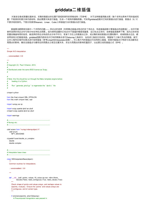
griddata⼆维插值 对某些设备或测量仪器来说,采集的数据点的位置不是规则排列的⽹格结构(可参考),对于这种数据⽤散点图(每个采样点具有不同的值或权重)不能很好的展⽰其内部结构,因此需要对其进⾏插值,⽣成⼀个规则的栅格图像。
可采⽤griddata函数对已知的数据点进⾏插值,数据点(X, Y)不要求规则排列。
下图分别使⽤Nearest、Linear、Cubic三种插值⽅法对数据点进⾏插值。
插值算法都要⾸先⾯对⼀个共同的问题—— 邻近点的选择(利⽤靠近插值点附近的多个邻近点,构造插值函数计算插值点的函数值)。
应尽可能使所选择的邻近点均匀地分布在待估点周围。
因为使⽤适量的已知点对于插值的精度很重要,当已知点过多时,会使插值准确率下降,因为过多的信息量会掩盖有⽤的信息;被选择的邻近点构成的点分布不均匀,若某个⽅位上的数据点过多,或点集的某些数据点位置较集中,或者数据点过远,都会带来较⼤的插值误差。
griddata函数内部会先对已知的数据点进⾏Delaunay三⾓剖分,当完成三⾓剖分完成后,根据每个三⾓⽚顶点的数值,就可以对三⾓形区域内任意点进⾏线性插值(参考LinearNDInterpolator函数)。
对三⾓⽚内的插值点可采⽤质⼼插值,即是对插值点只考虑与该点最邻近周围点的影响,确定出插值点与最邻近的周围点之相互位置关系,求出与周围点的影响权重因⼦,以此建⽴线性插值公式(参考)。
"""Simple N-D interpolation.. versionadded:: 0.9"""## Copyright (C) Pauli Virtanen, 2010.## Distributed under the same BSD license as Scipy.### Note: this file should be run through the Mako template engine before# feeding it to Cython.## Run ``generate_qhull.py`` to regenerate the ``qhull.c`` file#cimport cythonfrom libc.float cimport DBL_EPSILONfrom libc.math cimport fabs, sqrtimport numpy as npimport scipy.spatial.qhull as qhullcimport scipy.spatial.qhull as qhullimport warnings#------------------------------------------------------------------------------# Numpy etc.#------------------------------------------------------------------------------cdef extern from"numpy/ndarrayobject.h":cdef enum:NPY_MAXDIMSctypedef fused double_or_complex:doubledouble complex#------------------------------------------------------------------------------# Interpolator base class#------------------------------------------------------------------------------class NDInterpolatorBase(object):"""Common routines for interpolators... versionadded:: 0.9"""def__init__(self, points, values, fill_value=np.nan, ndim=None,rescale=False, need_contiguous=True, need_values=True):"""Check shape of points and values arrays, and reshape values to(npoints, nvalues). Ensure the `points` and values arrays areC-contiguous, and of correct type."""if isinstance(points, qhull.Delaunay):# Precomputed triangulation was passed inif rescale:raise ValueError("Rescaling is not supported when passing ""a Delaunay triangulation as ``points``.")self.tri = pointspoints = points.pointselse:self.tri = Nonepoints = _ndim_coords_from_arrays(points)values = np.asarray(values)_check_init_shape(points, values, ndim=ndim)if need_contiguous:points = np.ascontiguousarray(points, dtype=np.double)if need_values:self.values_shape = values.shape[1:]if values.ndim == 1:self.values = values[:,None]elif values.ndim == 2:self.values = valueselse:self.values = values.reshape(values.shape[0],np.prod(values.shape[1:]))# Complex or real?self.is_complex = np.issubdtype(self.values.dtype, plexfloating) if self.is_complex:if need_contiguous:self.values = np.ascontiguousarray(self.values,dtype=plex128)self.fill_value = complex(fill_value)else:if need_contiguous:self.values = np.ascontiguousarray(self.values, dtype=np.double) self.fill_value = float(fill_value)if not rescale:self.scale = Noneself.points = pointselse:# scale to unit cube centered at 0self.offset = np.mean(points, axis=0)self.points = points - self.offsetself.scale = self.points.ptp(axis=0)self.scale[~(self.scale > 0)] = 1.0 # avoid division by 0self.points /= self.scaledef _check_call_shape(self, xi):xi = np.asanyarray(xi)if xi.shape[-1] != self.points.shape[1]:raise ValueError("number of dimensions in xi does not match x")return xidef _scale_x(self, xi):if self.scale is None:return xielse:return (xi - self.offset) / self.scaledef__call__(self, *args):"""interpolator(xi)Evaluate interpolator at given points.Parameters----------x1, x2, ... xn: array-like of floatPoints where to interpolate data at.x1, x2, ... xn can be array-like of float with broadcastable shape.or x1 can be array-like of float with shape ``(..., ndim)``"""xi = _ndim_coords_from_arrays(args, ndim=self.points.shape[1])xi = self._check_call_shape(xi)shape = xi.shapexi = xi.reshape(-1, shape[-1])xi = np.ascontiguousarray(xi, dtype=np.double)xi = self._scale_x(xi)if self.is_complex:r = self._evaluate_complex(xi)else:r = self._evaluate_double(xi)return np.asarray(r).reshape(shape[:-1] + self.values_shape)cpdef _ndim_coords_from_arrays(points, ndim=None):"""Convert a tuple of coordinate arrays to a (..., ndim)-shaped array."""cdef ssize_t j, nif isinstance(points, tuple) and len(points) == 1:# handle argument tuplepoints = points[0]if isinstance(points, tuple):p = np.broadcast_arrays(*points)n = len(p)for j in range(1, n):if p[j].shape != p[0].shape:raise ValueError("coordinate arrays do not have the same shape") points = np.empty(p[0].shape + (len(points),), dtype=float) for j, item in enumerate(p):points[...,j] = itemelse:points = np.asanyarray(points)if points.ndim == 1:if ndim is None:points = points.reshape(-1, 1)else:points = points.reshape(-1, ndim)return pointscdef _check_init_shape(points, values, ndim=None):"""Check shape of points and values arrays"""if values.shape[0] != points.shape[0]:raise ValueError("different number of values and points")if points.ndim != 2:raise ValueError("invalid shape for input data points")if points.shape[1] < 2:raise ValueError("input data must be at least 2-D")if ndim is not None and points.shape[1] != ndim:raise ValueError("this mode of interpolation available only for ""%d-D data" % ndim)#------------------------------------------------------------------------------# Linear interpolation in N-D#------------------------------------------------------------------------------class LinearNDInterpolator(NDInterpolatorBase):"""LinearNDInterpolator(points, values, fill_value=np.nan, rescale=False)Piecewise linear interpolant in N dimensions... versionadded:: 0.9Methods-------__call__Parameters----------points : ndarray of floats, shape (npoints, ndims); or DelaunayData point coordinates, or a precomputed Delaunay triangulation.values : ndarray of float or complex, shape (npoints, ...)Data values.fill_value : float, optionalValue used to fill in for requested points outside of theconvex hull of the input points. If not provided, thenthe default is ``nan``.rescale : bool, optionalRescale points to unit cube before performing interpolation.This is useful if some of the input dimensions haveincommensurable units and differ by many orders of magnitude.Notes-----The interpolant is constructed by triangulating the input datawith Qhull [1]_, and on each triangle performing linearbarycentric interpolation.Examples--------We can interpolate values on a 2D plane:>>> from scipy.interpolate import LinearNDInterpolator>>> import matplotlib.pyplot as plt>>> np.random.seed(0)>>> x = np.random.random(10) - 0.5>>> y = np.random.random(10) - 0.5>>> z = np.hypot(x, y)>>> X = np.linspace(min(x), max(x))>>> Y = np.linspace(min(y), max(y))>>> X, Y = np.meshgrid(X, Y) # 2D grid for interpolation>>> interp = LinearNDInterpolator(list(zip(x, y)), z)>>> Z = interp(X, Y)>>> plt.pcolormesh(X, Y, Z, shading='auto')>>> plt.plot(x, y, "ok", label="input point")>>> plt.legend()>>> plt.colorbar()>>> plt.axis("equal")>>> plt.show()See also--------griddata :Interpolate unstructured D-D data.NearestNDInterpolator :Nearest-neighbor interpolation in N dimensions.CloughTocher2DInterpolator :Piecewise cubic, C1 smooth, curvature-minimizing interpolant in 2D. References----------.. [1] /"""def__init__(self, points, values, fill_value=np.nan, rescale=False):NDInterpolatorBase.__init__(self, points, values, fill_value=fill_value, rescale=rescale)if self.tri is None:self.tri = qhull.Delaunay(self.points)def _evaluate_double(self, xi):return self._do_evaluate(xi, 1.0)def _evaluate_complex(self, xi):return self._do_evaluate(xi, 1.0j)@cython.boundscheck(False)@cython.wraparound(False)def _do_evaluate(self, const double[:,::1] xi, double_or_complex dummy): cdef const double_or_complex[:,::1] values = self.valuescdef double_or_complex[:,::1] outcdef const double[:,::1] points = self.pointscdef const int[:,::1] simplices = self.tri.simplicescdef double c[NPY_MAXDIMS]cdef double_or_complex fill_valuecdef int i, j, k, m, ndim, isimplex, inside, start, nvaluescdef qhull.DelaunayInfo_t infocdef double eps, eps_broadndim = xi.shape[1]start = 0fill_value = self.fill_valueqhull._get_delaunay_info(&info, self.tri, 1, 0, 0)out = np.empty((xi.shape[0], self.values.shape[1]),dtype=self.values.dtype)nvalues = out.shape[1]eps = 100 * DBL_EPSILONeps_broad = sqrt(DBL_EPSILON)with nogil:for i in range(xi.shape[0]):# 1) Find the simplexisimplex = qhull._find_simplex(&info, c,&xi[0,0] + i*ndim,&start, eps, eps_broad)# 2) Linear barycentric interpolationif isimplex == -1:# don't extrapolatefor k in range(nvalues):out[i,k] = fill_valuecontinuefor k in range(nvalues):out[i,k] = 0for j in range(ndim+1):for k in range(nvalues):m = simplices[isimplex,j]out[i,k] = out[i,k] + c[j] * values[m,k]return out#------------------------------------------------------------------------------# Gradient estimation in 2D#------------------------------------------------------------------------------class GradientEstimationWarning(Warning):pass@cython.cdivision(True)cdef int _estimate_gradients_2d_global(qhull.DelaunayInfo_t *d, double *data, int maxiter, double tol,double *y) nogil:"""Estimate gradients of a function at the vertices of a 2d triangulation.Parameters----------info : inputTriangulation in 2Ddata : inputFunction values at the verticesmaxiter : inputMaximum number of Gauss-Seidel iterationstol : inputAbsolute / relative stop tolerancey : output, shape (npoints, 2)Derivatives [F_x, F_y] at the verticesReturns-------num_iterationsNumber of iterations if converged, 0 if maxiter reachedwithout convergenceNotes-----This routine uses a re-implementation of the global approximatecurvature minimization algorithm described in [Nielson83] and [Renka84]. References----------.. [Nielson83] G. Nielson,''A method for interpolating scattered data based upon a minimum norm network''.Math. Comp., 40, 253 (1983)... [Renka84] R. J. Renka and A. K. Cline.''A Triangle-based C1 interpolation method.'',Rocky Mountain J. Math., 14, 223 (1984)."""cdef double Q[2*2]cdef double s[2]cdef double r[2]cdef int ipoint, iiter, k, ipoint2, jpoint2cdef double f1, f2, df2, ex, ey, L, L3, det, err, change# initializefor ipoint in range(2*d.npoints):y[ipoint] = 0## Main point:## Z = sum_T sum_{E in T} int_E |W''|^2 = min!## where W'' is the second derivative of the Clough-Tocher# interpolant to the direction of the edge E in triangle T.## The minimization is done iteratively: for each vertex V,# the sum## Z_V = sum_{E connected to V} int_E |W''|^2## is minimized separately, using existing values at other V.## Since the interpolant can be written as## W(x) = f(x) + w(x)^T y## where y = [ F_x(V); F_y(V) ], it is clear that the solution to# the local problem is is given as a solution of the 2x2 matrix# equation.## Here, we use the Clough-Tocher interpolant, which restricted to# a single edge is## w(x) = (1 - x)**3 * f1# + x*(1 - x)**2 * (df1 + 3*f1)# + x**2*(1 - x) * (df2 + 3*f2)# + x**3 * f2## where f1, f2 are values at the vertices, and df1 and df2 are# derivatives along the edge (away from the vertices).## As a consequence, one finds## L^3 int_{E} |W''|^2 = y^T A y + 2 B y + C## with## A = [4, -2; -2, 4]# B = [6*(f1 - f2), 6*(f2 - f1)]# y = [df1, df2]# L = length of edge E## and C is not needed for minimization. Since df1 = dF1.E, df2 = -dF2.E, # with dF1 = [F_x(V_1), F_y(V_1)], and the edge vector E = V2 - V1,# we have## Z_V = dF1^T Q dF1 + 2 s.dF1 + const.## which is minimized by## dF1 = -Q^{-1} s## where## Q = sum_E [A_11 E E^T]/L_E^3 = 4 sum_E [E E^T]/L_E^3# s = sum_E [ B_1 + A_21 df2] E /L_E^3# = sum_E [ 6*(f1 - f2) + 2*(E.dF2)] E / L_E^3## Gauss-Seidelfor iiter in range(maxiter):err = 0for ipoint in range(d.npoints):for k in range(2*2):Q[k] = 0for k in range(2):s[k] = 0# walk over neighbours of given pointfor jpoint2 in range(d.vertex_neighbors_indptr[ipoint],d.vertex_neighbors_indptr[ipoint+1]):ipoint2 = d.vertex_neighbors_indices[jpoint2]# edgeex = d.points[2*ipoint2 + 0] - d.points[2*ipoint + 0]ey = d.points[2*ipoint2 + 1] - d.points[2*ipoint + 1]L = sqrt(ex**2 + ey**2)L3 = L*L*L# data at verticesf1 = data[ipoint]f2 = data[ipoint2]# scaled gradient projections on the edgedf2 = -ex*y[2*ipoint2 + 0] - ey*y[2*ipoint2 + 1]# edge sumQ[0] += 4*ex*ex / L3Q[1] += 4*ex*ey / L3Q[3] += 4*ey*ey / L3s[0] += (6*(f1 - f2) - 2*df2) * ex / L3s[1] += (6*(f1 - f2) - 2*df2) * ey / L3Q[2] = Q[1]# solvedet = Q[0]*Q[3] - Q[1]*Q[2]r[0] = ( Q[3]*s[0] - Q[1]*s[1])/detr[1] = (-Q[2]*s[0] + Q[0]*s[1])/detchange = max(fabs(y[2*ipoint + 0] + r[0]),fabs(y[2*ipoint + 1] + r[1]))y[2*ipoint + 0] = -r[0]y[2*ipoint + 1] = -r[1]# relative/absolute errorchange /= max(1.0, max(fabs(r[0]), fabs(r[1])))err = max(err, change)if err < tol:return iiter + 1# Didn't converge before maxiterreturn 0@cython.boundscheck(False)@cython.wraparound(False)cpdef estimate_gradients_2d_global(tri, y, int maxiter=400, double tol=1e-6): cdef const double[:,::1] datacdef double[:,:,::1] gradcdef qhull.DelaunayInfo_t infocdef int k, ret, nvaluesy = np.asanyarray(y)if y.shape[0] != tri.npoints:raise ValueError("'y' has a wrong number of items")if np.issubdtype(y.dtype, plexfloating):rg = estimate_gradients_2d_global(tri, y.real, maxiter=maxiter, tol=tol) ig = estimate_gradients_2d_global(tri, y.imag, maxiter=maxiter, tol=tol) r = np.zeros(rg.shape, dtype=complex)r.real = rgr.imag = igreturn ry_shape = y.shapeif y.ndim == 1:y = y[:,None]y = y.reshape(tri.npoints, -1).Ty = np.ascontiguousarray(y, dtype=np.double)yi = np.empty((y.shape[0], y.shape[1], 2))data = ygrad = yiqhull._get_delaunay_info(&info, tri, 0, 0, 1)nvalues = data.shape[0]for k in range(nvalues):with nogil:ret = _estimate_gradients_2d_global(&info,&data[k,0],maxiter,tol,&grad[k,0,0])if ret == 0:warnings.warn("Gradient estimation did not converge, ""the results may be inaccurate",GradientEstimationWarning)return yi.transpose(1, 0, 2).reshape(y_shape + (2,))#------------------------------------------------------------------------------# Cubic interpolation in 2D#------------------------------------------------------------------------------@cython.cdivision(True)cdef double_or_complex _clough_tocher_2d_single(qhull.DelaunayInfo_t *d, int isimplex,double *b,double_or_complex *f,double_or_complex *df) nogil:"""Evaluate Clough-Tocher interpolant on a 2D triangle.Parameters----------d :Delaunay infoisimplex : intTriangle to evaluate onb : shape (3,)Barycentric coordinates of the point on the trianglef : shape (3,)Function values at verticesdf : shape (3, 2)Gradient values at verticesReturns-------w :Value of the interpolant at the given pointReferences----------.. [CT] See, for example,P. Alfeld,''A trivariate Clough-Tocher scheme for tetrahedral data''.Computer Aided Geometric Design, 1, 169 (1984);G. Farin,''Triangular Bernstein-Bezier patches''.Computer Aided Geometric Design, 3, 83 (1986)."""cdef double_or_complex \c3000, c0300, c0030, c0003, \c2100, c2010, c2001, c0210, c0201, c0021, \c1200, c1020, c1002, c0120, c0102, c0012, \c1101, c1011, c0111cdef double_or_complex \f1, f2, f3, df12, df13, df21, df23, df31, df32cdef double g[3]cdef double \e12x, e12y, e23x, e23y, e31x, e31y, \e14x, e14y, e24x, e24y, e34x, e34ycdef double_or_complex wcdef double minvalcdef double b1, b2, b3, b4cdef int k, itricdef double c[3]cdef double y[2]# XXX: optimize + refactor this!e12x = (+ d.points[0 + 2*d.simplices[3*isimplex + 1]]- d.points[0 + 2*d.simplices[3*isimplex + 0]])e12y = (+ d.points[1 + 2*d.simplices[3*isimplex + 1]]- d.points[1 + 2*d.simplices[3*isimplex + 0]])e23x = (+ d.points[0 + 2*d.simplices[3*isimplex + 2]]- d.points[0 + 2*d.simplices[3*isimplex + 1]])e23y = (+ d.points[1 + 2*d.simplices[3*isimplex + 2]]- d.points[1 + 2*d.simplices[3*isimplex + 1]])e31x = (+ d.points[0 + 2*d.simplices[3*isimplex + 0]]- d.points[0 + 2*d.simplices[3*isimplex + 2]])e31y = (+ d.points[1 + 2*d.simplices[3*isimplex + 0]]- d.points[1 + 2*d.simplices[3*isimplex + 2]])e14x = (e12x - e31x)/3e14y = (e12y - e31y)/3e24x = (-e12x + e23x)/3e24y = (-e12y + e23y)/3e34x = (e31x - e23x)/3e34y = (e31y - e23y)/3f1 = f[0]f2 = f[1]f3 = f[2]df12 = +(df[2*0+0]*e12x + df[2*0+1]*e12y)df21 = -(df[2*1+0]*e12x + df[2*1+1]*e12y)df23 = +(df[2*1+0]*e23x + df[2*1+1]*e23y)df32 = -(df[2*2+0]*e23x + df[2*2+1]*e23y)df31 = +(df[2*2+0]*e31x + df[2*2+1]*e31y)df13 = -(df[2*0+0]*e31x + df[2*0+1]*e31y)c3000 = f1c2100 = (df12 + 3*c3000)/3c2010 = (df13 + 3*c3000)/3c0300 = f2c1200 = (df21 + 3*c0300)/3c0210 = (df23 + 3*c0300)/3c0030 = f3c1020 = (df31 + 3*c0030)/3c0120 = (df32 + 3*c0030)/3c2001 = (c2100 + c2010 + c3000)/3c0201 = (c1200 + c0300 + c0210)/3c0021 = (c1020 + c0120 + c0030)/3## Now, we need to impose the condition that the gradient of the spline # to some direction `w` is a linear function along the edge.## As long as two neighbouring triangles agree on the choice of the# direction `w`, this ensures global C1 differentiability.# Otherwise, the choice of the direction is arbitrary (except that# it should not point along the edge, of course).## In [CT]_, it is suggested to pick `w` as the normal of the edge.# This choice is given by the formulas## w_12 = E_24 + g[0] * E_23# w_23 = E_34 + g[1] * E_31# w_31 = E_14 + g[2] * E_12## g[0] = -(e24x*e23x + e24y*e23y) / (e23x**2 + e23y**2)# g[1] = -(e34x*e31x + e34y*e31y) / (e31x**2 + e31y**2)# g[2] = -(e14x*e12x + e14y*e12y) / (e12x**2 + e12y**2)## However, this choice gives an interpolant that is *not*# invariant under affine transforms. This has some bad# consequences: for a very narrow triangle, the spline can# develops huge oscillations. For instance, with the input data## [(0, 0), (0, 1), (eps, eps)], eps = 0.01# F = [0, 0, 1]# dF = [(0,0), (0,0), (0,0)]## one observes that as eps -> 0, the absolute maximum value of the # interpolant approaches infinity.## So below, we aim to pick affine invariant `g[k]`.# We choose## w = V_4' - V_4## where V_4 is the centroid of the current triangle, and V_4' the# centroid of the neighbour. Since this quantity transforms similarly # as the gradient under affine transforms, the resulting interpolant# is affine-invariant. Moreover, two neighbouring triangles clearly# always agree on the choice of `w` (sign is unimportant), and so# this choice also makes the interpolant C1.## The drawback here is a performance penalty, since we need to# peek into neighbouring triangles.#for k in range(3):itri = d.neighbors[3*isimplex + k]if itri == -1:# No neighbour.# Compute derivative to the centroid direction (e_12 + e_13)/2. g[k] = -1./2continue# Centroid of the neighbour, in our local barycentric coordinates y[0] = (+ d.points[0 + 2*d.simplices[3*itri + 0]]+ d.points[0 + 2*d.simplices[3*itri + 1]]+ d.points[0 + 2*d.simplices[3*itri + 2]]) / 3y[1] = (+ d.points[1 + 2*d.simplices[3*itri + 0]]+ d.points[1 + 2*d.simplices[3*itri + 1]]+ d.points[1 + 2*d.simplices[3*itri + 2]]) / 3qhull._barycentric_coordinates(2, d.transform + isimplex*2*3, y, c) # Rewrite V_4'-V_4 = const*[(V_4-V_2) + g_i*(V_3 - V_2)]# Now, observe that the results can be written *in terms of# barycentric coordinates*. Barycentric coordinates stay# invariant under affine transformations, so we can directly# conclude that the choice below is affine-invariant.if k == 0:g[k] = (2*c[2] + c[1] - 1) / (2 - 3*c[2] - 3*c[1])elif k == 1:g[k] = (2*c[0] + c[2] - 1) / (2 - 3*c[0] - 3*c[2])elif k == 2:g[k] = (2*c[1] + c[0] - 1) / (2 - 3*c[1] - 3*c[0])c0111 = (g[0]*(-c0300 + 3*c0210 - 3*c0120 + c0030)+ (-c0300 + 2*c0210 - c0120 + c0021 + c0201))/2c1011 = (g[1]*(-c0030 + 3*c1020 - 3*c2010 + c3000)+ (-c0030 + 2*c1020 - c2010 + c2001 + c0021))/2c1101 = (g[2]*(-c3000 + 3*c2100 - 3*c1200 + c0300)+ (-c3000 + 2*c2100 - c1200 + c2001 + c0201))/2c1002 = (c1101 + c1011 + c2001)/3c0102 = (c1101 + c0111 + c0201)/3c0012 = (c1011 + c0111 + c0021)/3c0003 = (c1002 + c0102 + c0012)/3# extended barycentric coordinatesminval = b[0]for k in range(3):if b[k] < minval:minval = b[k]b1 = b[0] - minvalb2 = b[1] - minvalb3 = b[2] - minvalb4 = 3*minval# evaluate the polynomial -- the stupid and ugly way to do it,# one of the 4 coordinates is in fact zerow = (b1**3*c3000 + 3*b1**2*b2*c2100 + 3*b1**2*b3*c2010 +3*b1**2*b4*c2001 + 3*b1*b2**2*c1200 +6*b1*b2*b4*c1101 + 3*b1*b3**2*c1020 + 6*b1*b3*b4*c1011 +3*b1*b4**2*c1002 + b2**3*c0300 + 3*b2**2*b3*c0210 +3*b2**2*b4*c0201 + 3*b2*b3**2*c0120 + 6*b2*b3*b4*c0111 +3*b2*b4**2*c0102 + b3**3*c0030 + 3*b3**2*b4*c0021 +3*b3*b4**2*c0012 + b4**3*c0003)return wclass CloughTocher2DInterpolator(NDInterpolatorBase):"""CloughTocher2DInterpolator(points, values, tol=1e-6)Piecewise cubic, C1 smooth, curvature-minimizing interpolant in 2D. .. versionadded:: 0.9Methods-------__call__Parameters----------points : ndarray of floats, shape (npoints, ndims); or DelaunayData point coordinates, or a precomputed Delaunay triangulation. values : ndarray of float or complex, shape (npoints, ...)Data values.fill_value : float, optionalValue used to fill in for requested points outside of theconvex hull of the input points. If not provided, thenthe default is ``nan``.tol : float, optionalAbsolute/relative tolerance for gradient estimation.maxiter : int, optionalMaximum number of iterations in gradient estimation.rescale : bool, optionalRescale points to unit cube before performing interpolation.This is useful if some of the input dimensions haveincommensurable units and differ by many orders of magnitude.Notes-----The interpolant is constructed by triangulating the input datawith Qhull [1]_, and constructing a piecewise cubicinterpolating Bezier polynomial on each triangle, using aClough-Tocher scheme [CT]_. The interpolant is guaranteed to becontinuously differentiable.The gradients of the interpolant are chosen so that the curvatureof the interpolating surface is approximatively minimized. Thegradients necessary for this are estimated using the globalalgorithm described in [Nielson83]_ and [Renka84]_.Examples--------We can interpolate values on a 2D plane:>>> from scipy.interpolate import CloughTocher2DInterpolator>>> import matplotlib.pyplot as plt>>> np.random.seed(0)>>> x = np.random.random(10) - 0.5>>> y = np.random.random(10) - 0.5>>> z = np.hypot(x, y)>>> X = np.linspace(min(x), max(x))>>> Y = np.linspace(min(y), max(y))>>> X, Y = np.meshgrid(X, Y) # 2D grid for interpolation>>> interp = CloughTocher2DInterpolator(list(zip(x, y)), z)>>> Z = interp(X, Y)>>> plt.pcolormesh(X, Y, Z, shading='auto')>>> plt.plot(x, y, "ok", label="input point")>>> plt.legend()>>> plt.colorbar()>>> plt.axis("equal")>>> plt.show()See also--------griddata :Interpolate unstructured D-D data.LinearNDInterpolator :Piecewise linear interpolant in N dimensions.NearestNDInterpolator :Nearest-neighbor interpolation in N dimensions.References----------.. [1] /.. [CT] See, for example,P. Alfeld,''A trivariate Clough-Tocher scheme for tetrahedral data''.Computer Aided Geometric Design, 1, 169 (1984);G. Farin,''Triangular Bernstein-Bezier patches''.Computer Aided Geometric Design, 3, 83 (1986)... [Nielson83] G. Nielson,''A method for interpolating scattered data based upon a minimum norm network''.Math. Comp., 40, 253 (1983)... [Renka84] R. J. Renka and A. K. Cline.''A Triangle-based C1 interpolation method.'',Rocky Mountain J. Math., 14, 223 (1984)."""def__init__(self, points, values, fill_value=np.nan,tol=1e-6, maxiter=400, rescale=False):NDInterpolatorBase.__init__(self, points, values, ndim=2,fill_value=fill_value, rescale=rescale)if self.tri is None:self.tri = qhull.Delaunay(self.points)self.grad = estimate_gradients_2d_global(self.tri, self.values,tol=tol, maxiter=maxiter)def _evaluate_double(self, xi):return self._do_evaluate(xi, 1.0)def _evaluate_complex(self, xi):return self._do_evaluate(xi, 1.0j)@cython.boundscheck(False)@cython.wraparound(False)def _do_evaluate(self, const double[:,::1] xi, double_or_complex dummy):cdef const double_or_complex[:,::1] values = self.valuescdef const double_or_complex[:,:,:] grad = self.gradcdef double_or_complex[:,::1] outcdef const double[:,::1] points = self.pointscdef const int[:,::1] simplices = self.tri.simplicescdef double c[NPY_MAXDIMS]cdef double_or_complex f[NPY_MAXDIMS+1]cdef double_or_complex df[2*NPY_MAXDIMS+2]cdef double_or_complex wcdef double_or_complex fill_valuecdef int i, j, k, m, ndim, isimplex, inside, start, nvaluescdef qhull.DelaunayInfo_t infocdef double eps, eps_broadndim = xi.shape[1]start = 0fill_value = self.fill_valueqhull._get_delaunay_info(&info, self.tri, 1, 1, 0)out = np.zeros((xi.shape[0], self.values.shape[1]),dtype=self.values.dtype)nvalues = out.shape[1]eps = 100 * DBL_EPSILONeps_broad = sqrt(eps)with nogil:for i in range(xi.shape[0]):# 1) Find the simplexisimplex = qhull._find_simplex(&info, c,&xi[i,0],&start, eps, eps_broad)# 2) Clough-Tocher interpolationif isimplex == -1:# outside triangulationfor k in range(nvalues):out[i,k] = fill_valuecontinuefor k in range(nvalues):for j in range(ndim+1):f[j] = values[simplices[isimplex,j],k]df[2*j] = grad[simplices[isimplex,j],k,0]df[2*j+1] = grad[simplices[isimplex,j],k,1]w = _clough_tocher_2d_single(&info, isimplex, c, f, df)out[i,k] = wreturn outView Code 下图中红⾊的是已知采样点,蓝⾊是待插值的栅格点,三⾓形内部栅格点的数值可通过线性插值或其它插值⽅法计算出,三⾓形外部的点可在函数中指定⼀个数值(默认为NaN)。
- 1、下载文档前请自行甄别文档内容的完整性,平台不提供额外的编辑、内容补充、找答案等附加服务。
- 2、"仅部分预览"的文档,不可在线预览部分如存在完整性等问题,可反馈申请退款(可完整预览的文档不适用该条件!)。
- 3、如文档侵犯您的权益,请联系客服反馈,我们会尽快为您处理(人工客服工作时间:9:00-18:30)。
arXiv:math/0008124v1 [math.CV] 16 Aug 2000
Silviu Olariu
∗பைடு நூலகம்
Institute of Physics and Nuclear Engineering, Department of Fundamental Experimental Physics 76900 Magurele, P.O. Box MG-6, Bucharest, Romania 4 August 2000
1 n ∞ k +pn /(k p=0 y
n−1 l=0 exp {y cos (2πl/n)}cos {y sin (2πl/n)
Abstract Polar commutative n-complex numbers of the form u = x0 + h1 x1 + h2 x2 + · · · + hn−1 xn−1 are introduced in n dimensions, the variables x0 , ..., xn−1 being real numbers. The polar n-complex number can be represented, in an even number of dimensions, by the modulus d, by the amplitude ρ, by 2 polar angles θ+ , θ− , by n/2 − 2 planar angles ψk−1 , and by n/2 − 1 azimuthal angles φk . In an odd number of dimensions, the polar n-complex number can be represented by d, ρ, by 1 polar angle θ+ , by (n − 3)/2 planar angles ψk−1 , and by (n − 1)/2 azimuthal angles φk . The exponential function of a polar n-complex number can be expanded in terms of the polar n-dimensional cosexponential functions gnk (y ), k = 0, 1, ..., n − 1. Expressions are given for these cosexponential functions. The polar n-complex numbers can be written in exponential and trigonometric forms with the aid of the modulus, amplitude and the angular variables. The polar n-complex functions defined by series of powers are analytic, and the partial derivatives of the components of the polar n-complex functions are closely related. The integrals of polar n-complex functions are independent of path in regions where the functions are regular. The fact that the exponential form of
1
Introduction
A regular, two-dimensional complex number x + iy can be represented geometrically by the modulus ρ = (x2 + y 2 )1/2 and by the polar angle θ = arctan(y/x). The modulus ρ is multiplicative and the polar angle θ is additive upon the multiplication of ordinary complex numbers. The quaternions of Hamilton are a system of hypercomplex numbers defined in four dimensions, the multiplication being a noncommutative operation, [1] and many other hypercomplex systems are possible, [2]-[4] but these hypercomplex systems do not have all the required properties of regular, two-dimensional complex numbers which rendered possible the development of the theory of functions of a complex variable. A system of complex numbers in n dimensions is described in this work, for which the multiplication is both associative and commutative, and which is rich enough in properties so that an exponential form exists and the concepts of analytic n-complex function, contour integration and residue can be defined. The n-complex numbers introduced in this work have the form u = x0 + h1 x1 + h2 x2 + · · · + hn−1 xn−1 , the variables x0 , ..., xn−1 being real numbers. The multiplication rules for the complex units h1 , ..., hn−1 are hj hk = hj +k if 0 ≤ j + k ≤ n − 1, and hj hk = hj +k−n if n ≤ j + k ≤ 2n − 2. The product of two n-complex numbers is equal to zero if both numbers are equal to zero, or if the numbers belong to certain n-dimensional hyperplanes described further in this work. If the n-complex number u = x0 + h1 x1 + h2 x2 + · · · + hn−1 xn−1 is represented by the point A of coordinates x0 , x1 , ..., xn−1 , the position of the point A can be described, in an
∗
e-mail: olariu@ifin.nipne.ro
1
a polar n-complex numbers depends on the cyclic variables φk leads to the concept of pole and residue for integrals on closed paths. The polynomials of polar n-complex variables can be written as products of linear or quadratic factors, although the factorization may not be unique.
1/2 , by n/2 − 1 2 2 even number of dimensions, by the modulus d = (x2 0 + x1 + · · · + xn−1 )
azimuthal angles φk , by n/2 − 2 planar angles ψk−1 , and by 2 polar angles θ+ , θ− . In an odd number of dimensions, the position of the point A is described by d, by (n − 1)/2 azimuthal
where v+ = x0 + · · · + xn−1 , v− = x0 − x1 + · · · + xn−2 − xn−1 , and ρk are radii in orthogonal two-dimensional planes defined further in this work. The amplitude ρ, the variables v+ , v− , √ √ the radii ρk , the variables (1/ 2) tan θ+ , (1/ 2) tan θ− , tan ψk−1 are multiplicative, and the azimuthal angles φk are additive upon the multiplication of n-complex numbers. Because of the role of the axis v+ and, in an even number of dimensions, of the axis v− , in the description of the position of the point A with the aid of the polar angle θ+ and, in an even number of dimensions, of the polar angle θ− , the hypercomplex numbers studied in this work will be called polar n-complex number, to distinguish them from the planar n-complex numbers, which exist in an even number of dimensions. [5] The exponential function of an n-complex number can be expanded in terms of the polar n-dimensional cosexponential functions gnk (y ) = 1. It is shown that gnk (y ) =