Chapter 10 Inferences on Two Samples - Kent State University:第10推测我们两样肯特州立大学
标准误excel计算公式
标准误excel计算公式英文回答:The standard error (SE) is a measure of the variability of a sample statistic. It is calculated by dividing the standard deviation of the sample by the square root of the sample size. The SE is used to make inferences about the population parameter that the sample statistic is estimating. For example, if we have a sample of 100 people and the sample mean is 50, then the SE of the sample meanis 5/sqrt(100) = 0.5. This means that we can be 95% confident that the population mean is between 49 and 51.The SE can also be used to compare the means of two samples. If we have two samples, each with a sample size of 100, and the sample means are 50 and 51, then the SE of the difference between the two sample means is sqrt(0.5^2 +0.5^2) = 0.71. This means that we can be 95% confident that the difference between the two population means is between -1.42 and 1.42.中文回答:标准误(SE)是样本统计量变异性的度量。
统计学CH10 英文版

We saw earlier that point probabilities in continuous distributions were virtually zero. Likewise, we’d expect that the point estimator gets closer to the parameter value with an increased sample size, but point estimators don’t reflect the effects of larger sample sizes. Hence we will employ the interval estimator to estimate population parameters…
Copyright © 2009 Cengage Learning
Unbiased Estimators…
An unbiased estimator of a population parameter is an estimator whose expected value is equal to that parameter. E.g. the sample median is an unbiased estimator of the population mean µ since: E(Sample median) = µ
To do so we need the population parameters. Binomial: p Poisson: µ Normal: µ and σ Exponential: λ or µ
Cop we have been…
Copyright © 2009 Cengage Learning
Solutions - Chapter 10

Solutions - Chapter 1010-1: Learning PythonOpen a blank file in your text editor and write a few lines summarizing what you’ve learned about Python so far. Start each line with the phrase In Python you can… Save the file as learning_python.txt in the same directory as your exercises fro mthis chapter. Write a program that reads the file and prints what you wrote three times. Print the contents once by reading in the entire file, once by looping over the file object, and once by storing the lines in a list and then working with them outside the with block.learning_python.txt:learning_python.py:Output:10-2: Learning CYou can use the replace() method to replace any word in a string with a different word. Here’s a quick example showing how to replace 'dog' with 'cat' in a sentence:Read in each line from the file you just created, learning_python.txt, and replace the word Python with the name of another language, such as C. Print each modified line to the screen.Output:You can use rstrip() and replace() on the same line. This iscalled chaining methods. In the following code the newline is stripped from the end of the line and then Python is replaced by C. The output is identical to the code shown above.10-3: GuestWrite a program that prompts the user for their name. When they respond, write their name to a file called guest.txt.Output:guest.txt:10-4: Guest BookWrite a while loop that prompts users for their name. When they entertheir name, print a greeting to the screen and add a line recording their visit in a file called guest_book.txt. Make sure each entry appears on a new line in the file.Output:guest_book.txt:10-5: Programming PollWrite a while loop that asks people why they like programming. Eachtime someone enters a reason, add their reason to a file that stores all the responses.Output:programming_poll.txt:10-6: AdditionOne common problem when prompting for numerical input occurs when people provide text instead of numbers. When you try to convert the input to an int, you’ll get a ValueError. Write a program that prompts for two numbers. Add them together and print the result. Catch the TypeError if either input value is not a number, and print a friendly error message. Test your program by entering two numbers and then by entering some text instead of a number.Output with two integers:Output with non-numerical input:10-7: Addition CalculatorWrap your code from Exercise 10-6 in a while loop so the user cancontinue entering numbers even if they make a mistake and enter text instead of a number.Output:10-8: Cats and DogsMake two files, cats.txt and dogs.txt. Store at least three names ofcats in the first file and three names of dogs in the second file. Write a program that tries to read these files and print the contents of the file to the screen. Wrap your code ina try-except block to catchthe FileNotFound error, and print a friendly message if a file is missing. Move one of the files to a different location on your system, and make sure the code in the except block executes properly.cats.txt:dogs.txt:cats_and_dogs.py:Output with both files:Output after moving cats.txt:10-9: Silent Cats and DogsModify your except block in Exercise 10-8 to fail silently if either file is missing.Output when both files exist:Output when cats.txt has been moved:10-11: Favorite NumberWrite a program that prompts for the user’s favorite number.Use json.dump() to store this number in a file. Write a separateprogram that reads in this value and prints the message, “I know your favorite number! It’s _____.”favorite_number_write.py:Output:favorite_number_read.py:Output:10-12: Favorite Number RememberedCombine the two programs from Exercise 10-11 into one file. If the number is already stored, report the favorite number to the user. If not, prompt for the user’s favorite number and store it in a file. Run the program twice to see that it works.Output, first run:Output, second run:10-13: Verify UserThe final listing for remember_me.py assumes either that the user has already entered their username or that the program is running for the first time. We should modify it in case the current user is not the person who last used the program.Before printing a welcome back message in greet_user(), ask the user if this is the correct username. If it’s not,call get_new_username() to get the correct username.Output:You might notice the identical else blocks in this versionof greet_user(). One way to clean this function up is to use an empty return statement. An empty return statement tells Python to leave the function without running any more code in the function. Here’s a cleaner version of greet_user():The return statement means the code in the function stops running after printing the welcome back message. When the username doesn’t exist, or the username is incorrect, the return statement is never reached. The second part of the function will only run whenthe if statements fail, so we don’t need an else block. Now the function prompts for a new username when either if statement fails. The only thing left to address is the nested if statements. This can be cleaned up by moving the code that checks whether the username iscorrect to a separate function. If you’re enjoying this exercise, you might try making a new function called check_username() and see if you can remove the nested if statement from greet_user().。
置信区间是一个随机区间
Learning Contents , Emphases and Difficulties
• • • • Confidence interval estimate [1] for one proportion [2] for one mean (or mean difference of pairs) [3] for difference between two means (unpooled) • [4] for difference between two means (pooled) • [5] for difference between two proportions (independent sample)
No:7 5/5/2009
10.1 The Language and Notation of Estimation P330
• 1.Unit: an individual person or object to be measured. • 2.Population (or universe): the entire collection of units about which we would like information or the entire collection of measurements we would have if we could measure the whole population. • 3.Sample: the collection of units we will actually measure or the collection of measurements we will actually obtain. • 4.Sample size: the number of units or measurements in the sample, denoted by n.
Chapter_1-1_
Statistics
Inferential Statistics
-methods
used to draw conclusions or inferences about characteristics of populations based on sample data.
2
Copyright © 2005 Brooks/Cole, a division of Thomson Learning, Inc.
Population standard deviation, is known Population standard deviation, is unknown and sample size, n 30.
t distribution
Population standard deviation, is unknown and sample size, n < 30.
Copyright © 2005 Brooks/Cole, a division of Thomson Learning, Inc.
10
The sample mean will be, for the most part, somewhat different from the population mean due to sampling error. So, how good is the point estimate? The answer is that, there is no way of knowing how close the point estimate is to the population mean. For this reason, statisticians prefer another type of estimate called an interval estimate.
elementary statistics 10th 解答
elementary statistics 10th 解答Elementary Statistics 10th Edition: An In-depth AnalysisIntroductionElementary Statistics is a fundamental branch of mathematics that deals with the collection, analysis, interpretation, presentation, and organization of data. In this article, we will delve into the various concepts covered in the 10th edition of Elementary Statistics, exploring topics such as data types, descriptive statistics, probability, hypothesis testing, and regression analysis. This comprehensive analysis aims to enhance the reader's understanding of statistics and its practical applications.Data Types and Sampling TechniquesIn elementary statistics, understanding different data types is crucial. The 10th edition explores the distinction between qualitative and quantitative data. Qualitative data refers to non-numeric information, such as names, labels, or categories. On the other hand, quantitative data represents numerical values that can be further classified as discrete or continuous. Discrete data consists of separate, countable values, while continuous data is measured on a continuous scale.Sampling techniques are also extensively discussed in the 10th edition of Elementary Statistics. Simple random sampling, stratified sampling, cluster sampling, and systematic sampling are explained in detail, along with their advantages and disadvantages. The book provides practical examples and exercises to strengthen the reader's comprehension of these sampling techniques.Descriptive Statistics: Measures of Central Tendency and DispersionDescriptive statistics allow statisticians to summarize and present data effectively. The 10th edition thoroughly covers measures of central tendency, including the mean, median, and mode. Each measure is defined and accompanied by clear examples and real-life applications. Additionally, the book introduces measures of dispersion, such as the range, variance, and standard deviation, to provide a comprehensive understanding of a dataset's variability.Probability and Probability DistributionsProbability theory plays a vital role in statistical analysis. The 10th edition delves into the basic concepts of probability, including the calculation of probabilities for various events. Concepts such as independent and dependent events, mutually exclusive events, and conditional probability are explained with clarity and simplicity.Furthermore, the book introduces probability distributions, focusing on the binomial and normal distributions. It discusses the properties and applications of these distributions, enabling readers to apply them in real-world scenarios. The explanations are accompanied by mathematical proofs and practical examples to enhance comprehension.Hypothesis Testing and Confidence IntervalsInferential statistics, particularly hypothesis testing, is an essential aspect of elementary statistics. The 10th edition provides a comprehensive explanation of hypothesis testing, including the formulation of null and alternative hypotheses, selection of significance levels, and determination oftest statistics. The book guides readers through various hypothesis tests, including tests for means, proportions, and variances, enabling them to make informed statistical decisions.Moreover, confidence intervals, which provide a range of plausible values for population parameters, are extensively covered in the 10th edition. The book explains the construction and interpretation of confidence intervals, empowering readers to make reliable estimations based on sample data.Regression Analysis and CorrelationRegression analysis is a powerful statistical technique used to model the relationship between two or more variables. The 10th edition introduces simple linear regression and multiple regression analysis, focusing on the interpretation of regression coefficients and the significance of the overall model. The book also explores correlation analysis, evaluating the strength and direction of the relationship between variables.Throughout the explanations of regression analysis and correlation, the 10th edition provides relevant examples and real-life applications to illustrate the practical implications of these statistical techniques.ConclusionThe 10th edition of Elementary Statistics offers a comprehensive and accessible approach to understanding statistics. It covers a wide range of topics, including data types, descriptive statistics, probability, hypothesis testing, regression analysis, and correlation. By providing clear explanations, real-life examples, and practical exercises, the book equips readers with the necessary knowledge and skills to apply statistical methods in various fields.Whether preparing for an exam or seeking a deeper understanding of statistics, this edition proves to be an invaluable resource for both students and professionals.。
ap06_stat_syllabus2
AP® StatisticsSyllabus 2Primary TextbookPeck, Roxy, Chris Olsen, and Jay Devore. Introduction to Statistics and Data Analysis, first edition. Pacific Grove, CA: Brooks/Cole, 2001. Technology [C5]•All students have a TI-83/TI-83+/TI-84 graphing calculator for use in class, at home, and on the AP Exam. Students will use theirgraphing calculator extensively throughout the course.•All students have a copy of JMP-Intro statistical software for use at home and for demonstrations in class. Students will haveoccasional assignments that must be completed using JMP-Intro.After the AP exam, students will use JMP-Intro daily when we learn multiple regression and ANOVA.•Various applets on the InternetCourse Outline(organized by chapters in primary textbook):Graphical displays include, but are not limited to using boxplots, dotplots, stemplots, back-to-back stemplots, histograms, frequency plots, parallel boxplots, and bar charts.Chapter 1: An Introduction to Statistics(total time: 1 day)•Activity: Sexual DiscriminationChapter 2: Collecting Data (total time: 14 days)[C2b]•Types of Data•Observational Studies•Activity: Sampling from the Gettysburg Address•Bias in sampling•Simple random samples•Stratified random samples•Activity: The River Problem•Cluster sampling•Designing experiments•Control groups•Treatments•Blocking• Random assignment • Replication• Activity: The Caffeine Experiment • The scope of inferenceChapter 3: Displaying Univariate Data (total time: 4 days) [C2a]•Displaying categorical data: pie and bar charts • Dotplots • Stemplots • Histograms• Describing the shape of a distribution • Cumulative frequency graphsChapter 4: Describing Univariate Data (total time: 8 days) [C2a] [C5]• Describing center: mean and median• Describing spread: range, interquartile range, and standard deviation • Boxplots • Outliers• Using the TI-83 • The empirical rule • Standardized scores • Percentiles and quartiles • Transforming data • Using JMP-Intro• Activity: Matching DistributionsChapter 5: Describing Bivariate Data (total time: 16 days) [C2a] [C5]• Introduction to bivariate data• Making and describing scatterplots • The correlation coefficient• Properties of the correlation coefficient • Least squares regression line • Using the TI-83• Regression to the mean • Residual plots• Standard deviation• Coefficient of determination •Unusual and influential points• Activity: Matching Scatterplots and Correlations • Applets: Demonstrating the effects of outliers • Using JMP-Intro• Modeling nonlinear data: exponential and power transformationsMidterm: Chapters 1–5 (total time: 3 days)• Review Chapters 1–5 using previous AP questions • Introduce first semester projectChapter 6: Probability (total time: 13 days) [C2c] [C5]• Definition of probability, outcomes, and events • Law of large numbers • Properties of probabilities • Conditional probability •Independence • Addition rule• Multiplication rule• Estimating probabilities using simulation • Using the TI-83 for simulations • Activity: Cereal Boxes • Activity: ESP Testing • Activity: Senior parkingChapter 7: Random Variables (total time: 18 days) [C2c] [C5]• Properties of discrete random variables • Properties of continuous random variables• Expected value (mean) of a discrete random variable • Standard deviation of a discrete random variable• Linear functions and linear combinations of random variables • The binomial distribution • The geometric distribution • The normal distribution • Using the normal table• Using the TI-83 distribution menu • Combining normal random variables • Normal approximation to the binomialFirst Semester Final Exam (total time: 4 days)• Review using previous AP questionsChapter 8: Sampling Distributions (total time: 9 days)[C2b]• Sampling distributions• Activity: How many textbooks?• Activity: Cents and the central limit theorem• Sampling distribution of the sample mean (including distribution of a difference between two independent sample means) • Sampling distribution of the sample proportion (including distribution of a difference between two independent sample proportions)Chapter 9: Confidence Intervals (total time: 10 days) [C2d]•Properties of point estimates: bias and variability • Confidence interval for a population proportion • Confidence interval for a population mean • Logic of confidence intervals • Meaning of confidence level• Activity: What does it mean to be 95% confident? •Finding sample size• Finite population correction factor • +4 confidence interval for a proportion • Confidence interval for a population mean • The t-distribution • Checking conditionsChapter 10: Hypothesis Tests (total time: 11 days) [C2d] [C5]• Forming hypotheses• Logic of hypothesis testing • Type I and Type II errors• Hypothesis test for a population proportion • Test statistics and p-values • Activity: Kissing the right way • Two-sided tests• Hypothesis test for a population mean • Checking conditions • Power• Using JMP-IntroChapter 11: Two Sample Procedures (total time: 11 days) [C2d] [C5]• Activity: Fish Oil• Hypothesis test for the difference of two means (unpaired) • Two-sided tests• Checking conditions• Confidence interval for the difference of two means (unpaired) • Matched pairs hypothesis test• Matched pairs confidence interval• Hypothesis test for the difference of two proportions • Confidence interval for the difference of two proportions • Using the TI-83 test menu• Choosing the correct test: It’s all about the designMidterm (chapters 8-11) (total time: 3 days)• Review using previous AP questionsChapter 12: Chi-square Tests (total time: 8 days) [C2d] [C5]• Activity: M&M’s• The chi-square distribution • Goodness of Fit test • Checking conditions •Assessing normality•Homogeneity of Proportions test (including large sample test for a proportion) • Using the TI-83• Test of independence• Choosing the correct test: It’s all about the design.Chapter 13: Inference for Slope (total time: 5 days)[C2d] [C5]• Activity: Dairy and Mucus• Hypothesis test for the slope of a least squares regression line • Confidence interval for the slope of a least squares regression line • Using the TI-83 • Using JMP-Intro• Understanding computer outputReview for AP Exam and Final Exam (total time: 7 days)• 2002 complete AP exam• Remaining previous AP questions • Final exam • AP examPost AP Exam (total time: 25 days)• Second semester project (see below) • Chapter 14: Multiple regression • Using JMP-Intro• Chapter 15: ANOVA • Using JMP-Intro•Guest speakers: careers in statisticsAP Statistics Example Project[[C2a, b, c, d]] [[C3]] [[C4]] [[C5]]The Project: Students will design and conduct an experiment toinvestigate the effects of response bias in surveys. They may choose the topic for their surveys, but they must design their experiment so that it can answer at least one of the following questions:•Can the wording of a question create response bias?• Do the characteristics of the interviewer create response bias? • Does anonymity change the responses to sensitive questions? • Does manipulating the answer choices change the response?The project will be done in pairs. Students will turn in one project per pair. A written report must be typed (single-spaced, 12-point font) and included graphs should be done on the computer using JMP-Intro or Excel.Proposal : The proposal should• Describe the topic and state which type of bias is being investigated.• Describe how to obtain subjects (minimum sample size is 50). • Describe what questions will be and how they will be asked, including how to incorporate direct control, blocking, and randomization.Written Report: The written report should include a title in the form of a question and the following sections (clearly labeled):• Introduction: What form of response bias was investigated? Whywas the topic chosen for the survey?• Methodology: Describe how the experiment was conducted and justify why the design was effective. Note: This section should be very similar to the proposal.• Results: Present the data in both tables and graphs in such a way that conclusions can be easily made. Make sure to label thegraphs/tables clearly and consistently.• Conclusions: What conclusions can be drawn from theexperiment? Be specific. Were any problems encountered during the project? What could be done different if the experiment were tobe repeated? What was learned from this project? • The original proposal.Poster: The poster should completely summarize the project, yet be simple enough to be understood by any reader. Students should include some pictures of the data collection in progress.Oral Presentation: Both members will participate equally. Theposter should be used as a visual aid. Students should be prepared for questions.。
788.Particulate Matter in Injection
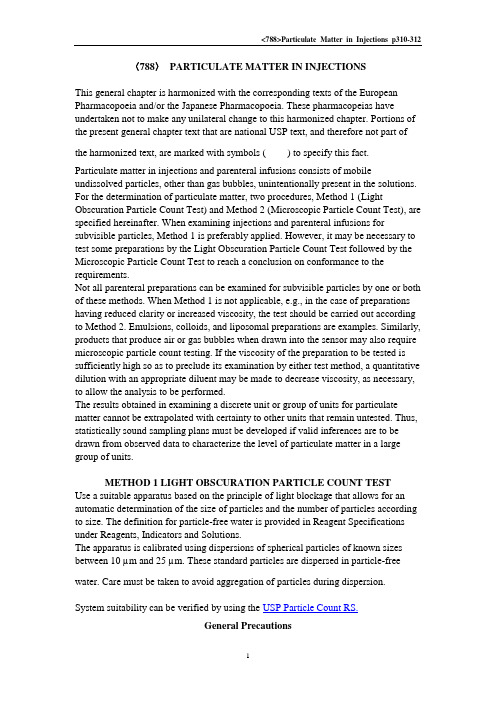
〈788〉PARTICULATE MATTER IN INJECTIONSThis general chapter is harmonized with the corresponding texts of the European Pharmacopoeia and/or the Japanese Pharmacopoeia. These pharmacopeias have undertaken not to make any unilateral change to this harmonized chapter. Portions of the present general chapter text that are national USP text, and therefore not part of the harmonized text, are marked with symbols () to specify this fact. Particulate matter in injections and parenteral infusions consists of mobile undissolved particles, other than gas bubbles, unintentionally present in the solutions. For the determination of particulate matter, two procedures, Method 1 (Light Obscuration Particle Count Test) and Method 2 (Microscopic Particle Count Test), are specified hereinafter. When examining injections and parenteral infusions for subvisible particles, Method 1 is preferably applied. However, it may be necessary to test some preparations by the Light Obscuration Particle Count Test followed by the Microscopic Particle Count Test to reach a conclusion on conformance to the requirements.Not all parenteral preparations can be examined for subvisible particles by one or both of these methods. When Method 1 is not applicable, e.g., in the case of preparations having reduced clarity or increased viscosity, the test should be carried out according to Method 2. Emulsions, colloids, and liposomal preparations are examples. Similarly, products that produce air or gas bubbles when drawn into the sensor may also require microscopic particle count testing. If the viscosity of the preparation to be tested is sufficiently high so as to preclude its examination by either test method, a quantitative dilution with an appropriate diluent may be made to decrease viscosity, as necessary, to allow the analysis to be performed.The results obtained in examining a discrete unit or group of units for particulate matter cannot be extrapolated with certainty to other units that remain untested. Thus, statistically sound sampling plans must be developed if valid inferences are to be drawn from observed data to characterize the level of particulate matter in a large group of units.METHOD 1 LIGHT OBSCURATION PARTICLE COUNT TESTUse a suitable apparatus based on the principle of light blockage that allows for an automatic determination of the size of particles and the number of particles according to size. The definition for particle-free water is provided in Reagent Specifications under Reagents, Indicators and Solutions.The apparatus is calibrated using dispersions of spherical particles of known sizes between 10 µm and 25 µm. These standard particles are dispersed in particle-free water. Care must be taken to avoid aggregation of particles during dispersion.System suitability can be verified by using the USP Particle Count RS.General PrecautionsThe test is carried out under conditions limiting particulate matter, preferably in a laminar flow cabinet.Very carefully wash the glassware and filtration equipment used, except for the membrane filters, with a warm detergent solution, and rinse with abundant amounts of water to remove all traces of detergent. Immediately before use, rinse the equipment from top to bottom, outside and then inside, with particle-free water.Take care not to introduce air bubbles into the preparation to be examined, especially when fractions of the preparation are being transferred to the container in which the determination is to be carried out.In order to check that the environment is suitable for the test, that the glassware is properly cleaned, and that the water to be used is particle-free, the following test is carried out: determine the particulate matter in 5 samples of particle-free water, each of 5 mL, according to the method described below. If the number of particles of 10µm or greater size exceeds 25 for the combined 25 mL, the precautions taken for the test are not sufficient. The preparatory steps must be repeated until the environment, glassware, and water are suitable for the test.MethodMix the contents of the sample by slowly inverting the container 20 times successively. If necessary, cautiously remove the sealing closure. Clean the outer surfaces of the container opening using a jet of particle-free water and remove the closure, avoiding any contamination of the contents. Eliminate gas bubbles by appropriate measures such as allowing to stand for 2 minutes or sonicating.For large-volume parenterals, single units are tested. For small-volume parenterals less than 25 mL in volume, the contents of 10 or more units are combined in a cleaned container to obtain a volume of not less than 25 mL; the test solution may be prepared by mixing the contents of a suitable number of vials and diluting to 25 mL with particle-free water or with an appropriate particle-free solvent when particle-free water is not suitable. Small-volume parenterals having a volume of 25 mL or more may be tested individually.Powders for parenteral use are reconstituted with particle-free water or with an appropriate particle-free solvent when particle-free water is not suitable.The number of test specimens must be adequate to provide a statistically sound assessment. For large-volume parenterals or for small-volume parenterals having a volume of 25 mL or more, fewer than 10 units may be tested, using an appropriate sampling plan.Remove four portions, not less than 5 mL each, and count the number of particles equal to or greater than 10 µm and 25 µm. Disregard the result obtained for the first portion, and calculate the mean number of particles for the preparation to be examined.EvaluationFor preparations supplied in containers with a nominal volume of more than 100 mL, apply the criteria of Test 1.A.For preparations supplied in containers with a nominal volume of less than 100 mL, apply the criteria of Test 1.B.For preparations supplied in containers with a nominal volume of 100 mL, apply the criteria of Test 1.B. [note—Test 1.A is used in the Japanese Pharmacopeia.]If the average number of particles exceeds the limits, test the preparation by the Microscopic Particle Count Test.Test 1.A (Solutions for parenteral infusion or solutions for injection supplied in containers with a nominal content of more than 100 mL)—The preparation complies with the test if the average number of particles present in the units tested does not exceed 25 per mL equal to or greater than 10 µm and does not exceed 3 per mL equal to or greater than 25 µm.Test 1.B (Solutions for parenteral infusion or solutions for injection supplied in containers with a nominal content of less than 100 mL)—The preparation complies with the test if the average number of particles present in the units tested does not exceed 6000 per container equal to or greater than 10 µm and does not exceed 600 per container equal to or greater than 25 µm.METHOD 2 MICROSCOPIC PARTICLE COUNT TESTUse a suitable binocular microscope, a filter assembly for retaining particulate matter, and a membrane filter for examination.The microscope is adjusted to 100 ± 10 magnifications and is equipped with an ocular micrometer calibrated with an objective micrometer, a mechanical stage capable of holding and traversing the entire filtration area of the membrane filter, and two suitable illuminators to provide episcopic illumination in addition to oblique illumination.The ocular micrometer is a circular diameter graticule (see Figure 1)Fig. 1. Circular diameter graticule. The large circle divided by crosshairs into quadrants is designated the graticule field of view (GFOV). Transparent and black circles having 10-µm and 25-µm diameters at 100× are provided as comparison scalesfor particle sizing.and consists of a large circle divided by crosshairs into quadrants, transparent and black reference circles 10 µm and 25 µm in diameter at 100 magnifications, and a linear scale graduated in 10-µm increments. It is calibrated using a stage micrometer that is certified by either a domestic or international standard institution. A relative error of the linear scale of the graticule within ±2% is acceptable. The large circle is designated the graticule field of view (GFOV).Two illuminators are required. One is an episcopic brightfield illuminator internal to the microscope, the other is an external, focusable auxiliary illuminator that can be adjusted to give reflected oblique illumination at an angle of 10to 20.The filter assembly for retaining particulate matter consists of a filter holder made of glass or other suitable material, and is equipped with a vacuum source and a suitable membrane filter.The membrane filter is of suitable size, black or dark gray in color, nongridded or gridded, and 1.0 µm or finer in nominal pore size.General PrecautionsThe test is carried out under conditions limiting particulate matter, preferably in a laminar flow cabinet.Very carefully wash the glassware and filter assembly used, except for the membrane filter, with a warm detergent solution, and rinse with abundant amounts of water to remove all traces of detergent. Immediately before use, rinse both sides of the membrane filter and the equipment from top to bottom, outside and then inside, with particle-free water.In order to check that the environment is suitable for the test, that the glassware and the membrane filter are properly cleaned, and that the water to be used is particle-free, the following test is carried out: determine the particulate matter of a 50-mL volume of particle-free water according to the method described below. If more than 20 particles 10 µm or larger in size or if more than 5 particles 25 µm or larger in size are present within the filtration area, the precautions taken for the test are not sufficient. The preparatory steps must be repeated until the environment, glassware, membrane filter, and water are suitable for the test.MethodMix the contents of the samples by slowly inverting the container 20 times successively. If necessary, cautiously remove the sealing closure. Clean the outer surfaces of the container opening using a jet of particle-free water and remove the closure, avoiding any contamination of the contents.For large-volume parenterals, single units are tested. For small-volume parenterals less than 25 mL in volume, the contents of 10 or more units are combined in a cleaned container; the test solution may be prepared by mixing the contents of a suitable number of vials and diluting to 25 mL with particle-free water or with an appropriate particle-free solvent when particle-free water is not suitable. Small-volume parenterals having a volume of 25 mL or more may be tested individually.Powders for parenteral use are constituted with particle-free water or with an appropriate particle-free solvent when particle-free water is not suitable.The number of test specimens must be adequate to provide a statistically sound assessment. For large-volume parenterals or for small-volume parenterals having a volume of 25 mL or more, fewer than 10 units may be tested, using an appropriate sampling plan.Wet the inside of the filter holder fitted with the membrane filter with several mL of particle-free water. Transfer to the filtration funnel the total volume of a solution pool or of a single unit, and apply a vacuum. If needed, add stepwise a portion of the solution until the entire volume is filtered. After the last addition of solution, begin rinsing the inner walls of the filter holder by using a jet of particle-free water. Maintain the vacuum until the surface of the membrane filter is free from liquid. Place the membrane filter in a Petri dish, and allow the membrane filter to air-dry with the cover slightly ajar. After the membrane filter has been dried, place the Petri dish on the stage of the microscope, scan the entire membrane filter under the reflected light from the illuminating device, and count the number of particles that are equal to or greater than 10 µm and the number of particles that are equal to or greater than 25 µm. Alternatively, partial membrane filter count and determination of the total filter count by calculation is allowed. Calculate the mean number of particles for the preparation to be examined.The particle sizing process with the use of the circular diameter graticule is carried out by estimating the equivalent diameter of the particle in comparison with the 10 µm and 25 µm reference circles on the graticule. Thereby the particles are not moved from their initial locations within the graticule field of view and are not superimposed on the reference circles for comparison. The inner diameter of the transparent graticule reference circles is used to size white and transparent particles, while dark particles are sized by using the outer diameter of the black opaque graticule reference circles.In performing the Microscopic Particle Count Test, do not attempt to size or enumerate amorphous, semiliquid, or otherwise morphologically indistinct materials that have the appearance of a stain or discoloration on the membrane filter. These materials show little or no surface relief and present a gelatinous or film-like appearance. In such cases, the interpretation of enumeration may be aided by testing a sample of the solution by the Light Obscuration Particle Count Test.EvaluationFor preparations supplied in containers with a nominal volume of more than 100 mL, apply the criteria of Test 2.A.For preparations supplied in containers with a nominal volume of less than 100 mL, apply the criteria of Test 2.B.For preparations supplied in containers with a nominal volume of 100 mL, apply the criteria of Test 2.B. [note—Test 2.A is used in the Japanese Pharmacopeia.]Test 2.A (Solutions for parenteral infusion or solutions for injection supplied in containers with a nominal content of more than 100 mL)—The preparation complies with the test if the average number of particles present in the units tested does not exceed 12 per mL equal to or greater than 10 µm and does not exceed 2 per mL equal to or greater than 25 µm.Test 2.B (Solutions for parenteral infusion or solutions for injection supplied in containers with a nominal content of less than 100 mL)—The preparation complies with the test if the average number of particles present in the units tested does not exceed 3000 per container equal to or greater than 10 µm and does not exceed 300 per container equal to or greater than 25 µm.。
- 1、下载文档前请自行甄别文档内容的完整性,平台不提供额外的编辑、内容补充、找答案等附加服务。
- 2、"仅部分预览"的文档,不可在线预览部分如存在完整性等问题,可反馈申请退款(可完整预览的文档不适用该条件!)。
- 3、如文档侵犯您的权益,请联系客服反馈,我们会尽快为您处理(人工客服工作时间:9:00-18:30)。
t
10.21
sd/ n 9.11/3
• Step 4. t is in the critical region. • Step 5. Conclusion:
No evidence support H0
EXAMPLE Constructing a Confidence Interval for the Mean Difference
• Step 1. Structure the Hypothesis
H0: u=0
H1: u ≠0
Step 2 give α=0.05
Critical values t=2.26216
C=(2.26216, infinity)
Step 3 Test Statistic d=31, s=9.11
d0 31
The degrees of freedom used to determine the critical value(s) presented in the last example are conservative.
Results that are more accurate can be obtained by using the following degrees of freedom:
In order to test the hypotheses regarding the mean difference, we need certain requirements to be satisfied.
• A simple random sample is obtained
• the sample data is matched pairs
(a) A researcher wants to know whether the price of a one night stay at a Holiday Inn Express Hotel is less than the price of a one night stay at a Red Roof Inn Hotel. She randomly selects 8 towns where the location of the hotels is close to each other and determines the price of a one night stay.
Construct a 90% confidence interval for the mean difference in price of Hampton Inn versus La Quinta hotel rooms.
Source: Expedia
Chapter 10 Inferences on Two Samples
(b) A researcher wants to know whether the newly issued “state” quarters have a mean weight that is different from “traditional” quarters. He randomly selects 18 “state” quarters and 16 “traditional” quarters. Their weights are compared.
Step 5 : State the conclusion.
EXAMPLE Testing a Claim Regarding Matched Pairs Data
Source: Expedia
Test Hypothesis
• Is the differences distribution normally distributed?
EXAMPLE Comparing Two Means: Independent Sampling
A researcher wanted to know whether “state” quarters had a weight that is more than “traditional” quarters. He randomly selected 18 “state” quarters and 16 “traditional” quarters, weighed each of them and obtained the following data.
Dependent samples are often referred to as matched pairs samples.
EXAMPLE Independent versus Dependent Sampling
For each of the following, determine whether the sampling method is independent or dependent.
Chapter 10 Inferences on Two Samples
10.1 Inference about Means:
Dependent Samd is independent when the individuals selected for one sample does not dictate which individuals are to be in a second sample. A sampling method is dependent when the individuals selected to be in one sample are used to determine the individuals to be in the second sample.
Construct a 95% confidence interval about the difference between the weight of “state” quarters and “traditional” quarters.
• the differences are normally distributed or the sample size, n, is large (n > 30).
Step 4: Compare the critical value with the test statistic:
Lower Bound =
(x1 x2)t/2
s12 s22 n1 n2
Upper Bound = (x1x2)t/2
s12 s22 n1 n2
EXAMPLE Constructing a Confidence Interval about the Difference of Two Means
10.2 Inference about Two Means:
Independent Sampling
Step 4: Compare the critical value with the test statistic:
Step 5 : State the conclusion.