
Phase transitions and configuration space topology
2 among a considerable number of publications and, second, several of the results, although correct, demand a reinterpretation as a consequence of recent findings and developments. The purpose of the present paper is to assemble from the known results, as far as possible, a coherent picture of the relation between phase transitions and configuration space topology, and to indicate new lines of research which might open up from these concepts. thermodynamic function leads to a discontinuity or to a divergence in some derivative of this function, and this is a typical signature of a phase transition as measured experimentally. Within the (grand)canonical ensemble of statistical mechanics, such a nonanalytic behavior can occur only in the thermodynamic limit, in which the number of degrees of freedom N of the system goes to infinity.2 Conceptually, the necessity of the thermodynamic limit is an objectionable feature: first, the number of degrees of freedom in real systems, although possibly large, is finite, and, second, for systems with long-range interactions, the thermodynamic limit may even be not well defined. These observations indicate that the theoretical description of phase transitions, although very successful in certain aspects, may not be completely satisfactory. Apart from this conceptual shortcoming, in the field of phase transitions there are many problems of applied nature which are far from being settled. One of those is the search for sufficient or necessary conditions for the occurrence of a phase transition. Among the necessary conditions for the occurrence of a phase transition, there are some of reasonable generality, like the MerminWagner theorem and its generalizations (Fannes et al., 1984; Fr¨ ohlich and Pfister, 1981; Mermin and Wagner, 1966) or the theorems on the absence of phase transitions in certain one-dimensional systems by van Hove (1950) and by Cuesta and S´ anchez (2004). Yet improved criteria are of course desirable. Less is known about conditions sufficient to guarantee a phase transition to take place. The Peierls argument (Peierls, 1936) or the Fr¨ ohlich-Simon-Spencer bound (Fr¨ ohlich et al., 1976) can be used to prove the existence of phase transitions without explicitly computing a thermodynamic potential, but their application is model specific and may be difficult depending on the system of interest. The above considerations motivate a further study on the “nature” of phase transitions, of the underlying mechanisms leading to a nonanalytic point of a thermodynamic function, and of the conditions under which they can occur. A classic result identifying such a nonanalyticity generating mechanism is the seminal theorem of Lee and Yang, relating the properties of the zeros of the grandcanonical partition function in the complex fugacity plane to nonanalyticities of the corresponding thermodynamic function (Lee and Yang, 1952). The main issue of the present paper is to investigate the mechanism which is at the basis of a phase transition using a different approach, based on concepts from differential geometry and topology. This topological approach emerged from the study of Hamiltonian dynamical systems and is therefore—at least in its present formulation—applicable to classical (i. e., nonquantum mechanical) systems. Hamiltonian
Contents
Preface I. Introduction II. Definitions and preliminaries A. Standard Hamiltonian systems B. Configuration space subsets C. Thermodynamic functions 1. Microcanonical thermodynamic functions 2. Canonical thermodynamic functions 3. Relation of microcanonical and canonical thermodynamic functions D. Nonanalytic points and phase transitions III. Computation of topological quantities A. Morse theory B. Model calculation: Mean-field k -trigonometric model C. Numerical computation of topological quantities 1. Euler characteristic via Gauss-Bonnet theorem 2. Critical points of the potential IV. Nonanalyticities in finite systems V. Phase transitions and configuration space topology A. Conjectures B. Franzosi-Pettini theorem C. Models not covered by Theorem V.7 VI. Limitations of the relation between phase transitions and configuration space topology A. Long-range interactions B. Nonconfining potentials 1 2 3 3 4 4 4 4 5 5 6 6 7 8 8 9 9 10 10 11 12 12 12 14
Phase transitions and configuration space topology
Michael Kastner∗
Pushingthelimits
3
FEEL THE SPEED.
Faster and further: The dynamic motors accelerate the wheelchair up to 6 km/h (optionally 10 km/h*). So you can really get going and enjoy the ride. The efficient energy recovery system feeds energy back into the batteries during braking, providing a 10 % range extension for greater freedom.
So it‘s even more logical that Alber also offers its service digitally. Simply download the twion Mobility App at no cost from Google Play Store onto all android-capable smartphones and use the all-round service at any time. For example, if service is required the diagnostic checklist can help to localise the error in the wheels and, if necessary, set up direct contact to our Service Team.
XC7VX690T-1FFG1927C
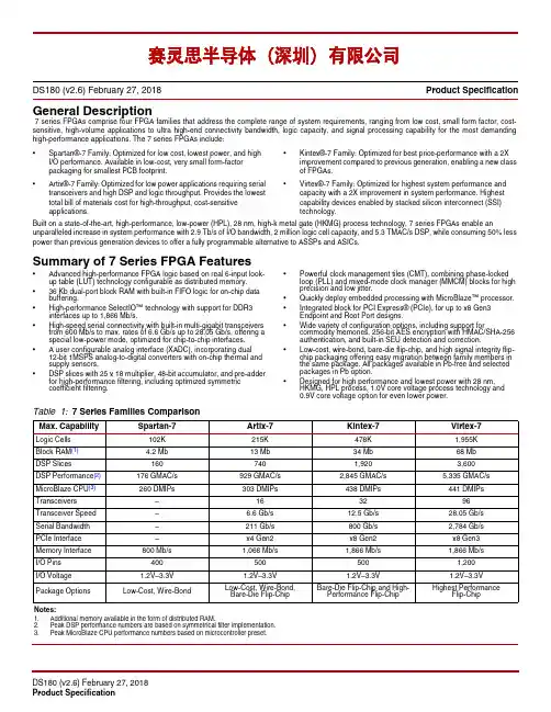
General Description7series FPGAs comprise four FPGA families that address the complete range of system requirements, ranging from low cost, small form factor, cost-sensitive, high-volume applications to ultra high-end connectivity bandwidth, logic capacity, and signal processing capability for the most demanding high-performance applications. The 7series FPGAs include:•Spartan®-7 Family: Optimized for low cost, lowest power, and high I/O performance. Available in low-cost, very small form-factorpackaging for smallest PCB footprint.•Artix®-7 Family: Optimized for low power applications requiring serial transceivers and high DSP and logic throughput. Provides the lowest total bill of materials cost for high-throughput, cost-sensitiveapplications.•Kintex®-7 Family: Optimized for best price-performance with a 2X improvement compared to previous generation, enabling a new class of FPGAs.•Virtex®-7 Family: Optimized for highest system performance and capacity with a 2X improvement in system performance. Highestcapability devices enabled by stacked silicon interconnect (SSI)technology.Built on a state-of-the-art, high-performance, low-power (HPL), 28nm, high-k metal gate (HKMG) process technology, 7series FPGAs enable an unparalleled increase in system performance with 2.9Tb/s of I/O bandwidth, 2 million logic cell capacity, and 5.3TMAC/s DSP, while consuming 50% less power than previous generation devices to offer a fully programmable alternative to ASSPs and ASICs.Summary of 7Series FPGA Features•Advanced high-performance FPGA logic based on real 6-input look-up table (LUT) technology configurable as distributed memory.•36Kb dual-port block RAM with built-in FIFO logic for on-chip data buffering.•High-performance SelectIO™ technology with support for DDR3 interfaces up to 1,866 Mb/s.•High-speed serial connectivity with built-in multi-gigabit transceivers from 600Mb/s to max. rates of 6.6Gb/s up to 28.05Gb/s, offering a special low-power mode, optimized for chip-to-chip interfaces.• A user configurable analog interface (XADC), incorporating dual 12-bit 1MSPS analog-to-digital converters with on-chip thermal and supply sensors.•DSP slices with 25x18 multiplier, 48-bit accumulator, and pre-adder for high-performance filtering, including optimized symmetriccoefficient filtering.•Powerful clock management tiles (CMT), combining phase-locked loop (PLL) and mixed-mode clock manager (MMCM) blocks for high precision and low jitter.•Quickly deploy embedded processing with MicroBlaze™ processor.•Integrated block for PCI Express® (PCIe), for up to x8 Gen3 Endpoint and Root Port designs.•Wide variety of configuration options, including support for commodity memories, 256-bit AES encryption with HMAC/SHA-256 authentication, and built-in SEU detection and correction.•Low-cost, wire-bond, bare-die flip-chip, and high signal integrity flip-chip packaging offering easy migration between family members in the same package. All packages available in Pb-free and selected packages in Pb option.•Designed for high performance and lowest power with 28nm, HKMG, HPL process, 1.0V core voltage process technology and0.9V core voltage option for even lower power.DS180 (v2.6) February 27, 2018Product SpecificationTable 1:7Series Families ComparisonMax. Capability Spartan-7Artix-7Kintex-7Virtex-7Logic Cells102K215K478K1,955KBlock RAM(1) 4.2Mb13Mb34Mb68MbDSP Slices 1607401,9203,600DSP Performance(2)176 GMAC/s929GMAC/s2,845GMAC/s5,335GMAC/s MicroBlaze CPU(3)260 DMIPs303 DMIPs438 DMIPs441 DMIPs Transceivers–163296Transceiver Speed– 6.6Gb/s12.5Gb/s28.05Gb/sSerial Bandwidth–211Gb/s800Gb/s2,784Gb/sPCIe Interface–x4 Gen2x8 Gen2x8 Gen3Memory Interface800Mb/s1,066Mb/s1,866Mb/s1,866Mb/sI/O Pins400500500 1,200I/O Voltage 1.2V–3.3V 1.2V–3.3V 1.2V–3.3V 1.2V–3.3VPackage Options Low-Cost, Wire-Bond Low-Cost, Wire-Bond,Bare-Die Flip-Chip Bare-Die Flip-Chip and High-Performance Flip-ChipHighest PerformanceFlip-ChipNotes:1.Additional memory available in the form of distributed RAM.2.Peak DSP performance numbers are based on symmetrical filter implementation.3.Peak MicroBlaze CPU performance numbers based on microcontroller preset.赛灵思半导体(深圳)有限公司质量等级领域:宇航级IC、特军级IC、超军级IC、普军级IC、禁运IC、工业级IC,军级二三极管,功率管等;应用领域:航空航天、船舶、汽车电子、军用计算机、铁路、医疗电子、通信网络、电力工业以及大型工业设备祝您:工作顺利,生活愉快!以赛灵思半导体(深圳)有限公司提供的参数为例,以下为XC7VX690T-1FFG1927C的详细参数,仅供参考赛灵思半导体(深圳)有限公司Stacked Silicon Interconnect (SSI) TechnologyThere are many challenges associated with creating high capacity FPGAs that Xilinx addresses with the SSI technology. SSI technology enables multiple super logic regions (SLRs) to be combined on a passive interposer layer, using proven manufacturing and assembly techniques from industry leaders, to create a single FPGA with more than ten thousand inter-SLR connections, providing ultra-high bandwidth connectivity with low latency and low power consumption. There are two types of SLRs used in Virtex-7 FPGAs: a logic intensive SLR used in the Virtex-7 T devices and a DSP/blockRAM/transceiver-rich SLR used in the Virtex-7 XT and HT devices. SSI technology enables the production of highercapability FPGAs than traditional manufacturing methods, enabling the highest capacity and highest performance FPGAs ever created to reach production more quickly and with less risk than would otherwise be possible. Thousands of super long line (SLL) routing resources and ultra-high performance clock lines that cross between the SLRs ensure that designs span seamlessly across these high-density programmable logic devices.CLBs, Slices, and LUTsSome key features of the CLB architecture include: •Real 6-input look-up tables (LUTs)•Memory capability within the LUT •Register and shift register functionalityThe LUTs in 7 series FPGAs can be configured as either one 6-input LUT (64-bit ROMs) with one output, or as two 5-input LUTs (32-bit ROMs) with separate outputs but common addresses or logic inputs. Each LUT output can optionally be registered in a flip-flop. Four such LUTs and their eight flip-flops as well as multiplexers and arithmetic carry logic form a slice, and two slices form a configurable logic block (CLB). Four of the eight flip-flops per slice (one per LUT) can optionally be configured as latches.Between 25–50% of all slices can also use their LUTs as distributed 64-bit RAM or as 32-bit shift registers (SRL32) or as two SRL16s. Modern synthesis tools take advantage of these highly efficient logic, arithmetic, and memory features.Clock ManagementSome of the key highlights of the clock management architecture include:•High-speed buffers and routing for low-skew clock distribution •Frequency synthesis and phase shifting •Low-jitter clock generation and jitter filteringEach 7series FPGA has up to 24 clock management tiles (CMTs), each consisting of one mixed-mode clock manager (MMCM)and one phase-locked loop (PLL).Table 11:Virtex-7 HT FPGA Device-Package Combinations and Maximum I/OsPackage (1)FLG1155FLG1931FLG1932Size (mm)35 x 3545 x 4545 x 45Ball Pitch 1.0 1.0 1.0Device GTH GTZ I/O GTH GTZ I/O GTHGTZI/O HP (2)HP (2)HP (2)XC7VH580T 248400488600XC7VH870T7216300Notes: 1.All packages listed are Pb-free with exemption 15. Some packages are available in Pb option.2.HP = High-performance I/O with support for I/O voltage from 1.2V to 1.8V.LC tank or, in the case of the GTZ, a single LC tank architecture to allow the ideal blend of flexibility and performance while enabling IP portability across the family members. The different 7series family members offer different top-end data rates. The GTP operates up to 6.6Gb/s, the GTX operates up to 12.5Gb/s, the GTH operates up to 13.1Gb/s, and the GTZ operates up to 28.05Gb/s. Lower data rates can be achieved using FPGA logic-based oversampling. The serial transmitter and receiver are independent circuits that use an advanced PLL architecture to multiply the reference frequency input by certain programmable numbers up to 100 to become the bit-serial data clock. Each transceiver has a large number of user-definable features and parameters. All of these can be defined during device configuration, and many can also be modified during operation.TransmitterThe transmitter is fundamentally a parallel-to-serial converter with a conversion ratio of 16, 20, 32, 40, 64, or 80. Additionally, the GTZ transmitter supports up to 160 bit data widths. This allows the designer to trade-off datapath width for timing margin in high-performance designs. These transmitter outputs drive the PC board with a single-channel differential output signal. TXOUTCLK is the appropriately divided serial data clock and can be used directly to register the parallel data coming from the internal logic. The incoming parallel data is fed through an optional FIFO and has additional hardware support for the 8B/10B, 64B/66B, or 64B/67B encoding schemes to provide a sufficient number of transitions. The bit-serial output signal drives two package pins with differential signals. This output signal pair has programmable signal swing as well as programmable pre- and post-emphasis to compensate for PC board losses and other interconnect characteristics. For shorter channels, the swing can be reduced to reduce power consumption.ReceiverThe receiver is fundamentally a serial-to-parallel converter, changing the incoming bit-serial differential signal into a parallel stream of words, each 16, 20, 32, 40, 64, or 80 bits. Additionally, the GTZ receiver supports up to 160 bit data widths. This allows the FPGA designer to trade-off internal datapath width versus logic timing margin.The receiver takes the incoming differential data stream, feeds it through programmable linear and decision feedback equalizers (to compensate for PC board and other interconnect characteristics), and uses the reference clock input to initiate clock recognition. There is no need for a separate clock line. The data pattern uses non-return-to-zero (NRZ) encoding and optionally guarantees sufficient data transitions by using the selected encoding scheme. Parallel data is then transferred into the FPGA logic using the RXUSRCLK clock. For short channels, the transceivers offers a special low power mode (LPM) to reduce power consumption by approximately 30%.Out-of-Band SignalingThe transceivers provide out-of-band (OOB) signaling, often used to send low-speed signals from the transmitter to the receiver while high-speed serial data transmission is not active. This is typically done when the link is in a powered-down state or has not yet been initialized. This benefits PCI Express and SATA/SAS applications.Integrated Interface Blocks for PCI Express DesignsHighlights of the integrated blocks for PCI Express include:•Compliant to the PCI Express Base Specification 2.1 or 3.0 (depending of family) with Endpoint and Root Port capability•Supports Gen1 (2.5Gb/s), Gen2 (5Gb/s), and Gen3 (8Gb/s) depending on device family•Advanced configuration options, Advanced Error Reporting (AER), and End-to-End CRC (ECRC) Advanced Error Reporting and ECRC features•Multiple-function and single root I/O virtualization (SR-IOV) support enabled through soft-logic wrappers or embedded in the integrated block depending on familyAll Artix-7, Kintex-7, and Virtex-7 devices include at least one integrated block for PCI Express technology that can be configured as an Endpoint or Root Port, compliant to the PCI Express Base Specification Revision 2.1 or 3.0. The Root Port can be used to build the basis for a compatible Root Complex, to allow custom FPGA-to-FPGA communication via the PCI Express protocol, and to attach ASSP Endpoint devices, such as Ethernet Controllers or Fibre Channel HBAs, to the FPGA. This block is highly configurable to system design requirements and can operate 1, 2, 4, or 8 lanes at the 2.5 Gb/s, 5.0 Gb/s, and 8.0Gb/s data rates. For high-performance applications, advanced buffering techniques of the block offer a flexible赛灵思半导体(深圳)有限公司7Series FPGAs Data Sheet: Overview。
38.300-无线接入网(NG-RAN)概述和总体描述英文原版

38.300-⽆线接⼊⽹(NG-RAN)概述和总体描述英⽂原版3GPP TS38.300V15.5.0(2019-03)Technical Specification3rd Generation Partnership Project;Technical Specification Group Radio Access Network;NR;NR and NG-RAN Overall Description;Stage2(Release15)The present document has been developed within the3rd Generation Partnership Project(3GPP TM)and may be further elaborated for the purposes of3GPP. The present document has not been subject to any approval process by the3GPP Organizational Partners and shall not be implemented.This Specification is provided for future development work within3GPP only.The Organizational Partners accept no liability for any use of this Specification. Specifications and Reports for implementation of the3GPP TM system should be obtained via the3GPP Organizational Partners'Publications Offices.3GPPPostal address3GPP support office address650Route des Lucioles-Sophia AntipolisValbonne-FRANCETel.:+33492944200Fax:+33493654716Internet/doc/2e6bf4e527c52cc58bd63186bceb19e8b8f6ecf2.htmlCopyright NotificationNo part may be reproduced except as authorized by written permission.The copyright and the foregoing restriction extend to reproduction in all media.2019,3GPP Organizational Partners(ARIB,ATIS,CCSA,ETSI,TSDSI,TTA,TTC).All rights reserved.UMTS?is a Trade Mark of ETSI registered for the benefit of its members3GPP?is a Trade Mark of ETSI registered for the benefit of its Members and of the3GPP Organizational Partners LTE?is a Trade Mark of ETSI registered for the benefit of its Members and of the3GPP Organizational Partners GSM?and the GSM logo are registered and owned by the GSM AssociationContentsForeword (7)1Scope (8)2References (8)3Abbreviations and Definitions (9)3.1Abbreviations (9)3.2Definitions (11)4Overall Architecture and Functional Split (11)4.1Overall Architecture (11)4.2Functional Split (12)4.3Network Interfaces (14)4.3.1.1NG User Plane (14)4.3.1.2NG Control Plane (14)4.3.2Xn Interface (15)4.3.2.1Xn User Plane (15)4.3.2.2Xn Control Plane (16)4.4Radio Protocol Architecture (16)4.4.1User Plane (16)4.4.2Control Plane (17)4.5Multi-Radio Dual Connectivity (17)5Physical Layer (17)5.1Waveform,numerology and frame structure (17)5.2Downlink (18)5.2.1Downlink transmission scheme (18)5.2.2Physical-layer processing for physical downlink shared channel (18) 5.2.3Physical downlink control channels (19)5.2.4Synchronization signal and PBCH block (20)5.2.5Physical layer procedures (20)5.2.5.1Link adaptation (20)5.2.5.2Power Control (21)5.2.5.3Cell search (21)5.2.5.4HARQ (21)5.2.5.5Reception of SIB1 (21)5.3Uplink (21)5.3.1Uplink transmission scheme (21)5.3.2Physical-layer processing for physical uplink shared channel (22) 5.3.3Physical uplink control channel (22)5.3.4Random access (23)5.3.5Physical layer procedures (23)5.3.5.1Link adaptation (23)5.3.5.2Uplink Power control (23)5.3.5.3Uplink timing control (23)5.3.5.4HARQ (24)5.4Carrier aggregation (24)5.4.1Carrier aggregation (24)5.4.2Supplementary Uplink (24)5.5Transport Channels (24)6Layer2 (25)6.1Overview (25)6.2MAC Sublayer (27)6.2.1Services and Functions (27)6.2.2Logical Channels (27)6.2.3Mapping to Transport Channels (27)6.3RLC Sublayer (28)6.3.1Transmission Modes (28)6.3.2Services and Functions (28)6.3.3ARQ (28)6.4PDCP Sublayer (29)6.4.1Services and Functions (29)6.5SDAP Sublayer (29)6.6L2Data Flow (29)6.7Carrier Aggregation (30)6.8Dual Connectivity (31)6.9Supplementary Uplink (31)6.10Bandwidth Adaptation (31)7RRC (32)7.1Services and Functions (32)7.3System Information Handling (33)7.3.1Overview (33)7.3.2Scheduling (35)7.3.3SI Modification (35)7.4Access Control (35)7.5UE Capability Retrieval framework (35)7.6Transport of NAS Messages (36)7.7Carrier Aggregation (36)7.8Bandwidth Adaptation (36)7.9UE Assistance Information (36)8NG Identities (36)8.1UE Identities (36)8.2Network Identities (37)9Mobility and State Transitions (37)9.1Overview (37)9.2Intra-NR (38)9.2.1Mobility in RRC_IDLE (38)9.2.1.1Cell Selection (38)9.2.1.2Cell Reselection (39)9.2.1.3State Transitions (39)9.2.2Mobility in RRC_INACTIVE (41)9.2.2.1Overview (41)9.2.2.2Cell Reselection (42)9.2.2.3RAN-Based Notification Area (42)9.2.2.4State Transitions (42)9.2.2.4.1UE triggered transition from RRC_INACTIVE to RRC_CONNECTED (42)9.2.2.4.2Network triggered transition from RRC_INACTIVE to RRC_CONNECTED (44) 9.2.2.5RNA update (45)9.2.3Mobility in RRC_CONNECTED (47)9.2.3.1Overview (47)9.2.3.2Handover (48)9.2.3.2.1C-Plane Handling (48)9.2.3.2.2U-Plane Handling (50)9.2.3.2.3Data Forwarding (52)9.2.3.3Re-establishment procedure (53)9.2.4Measurements (53)9.2.5Paging (56)9.2.6Random Access Procedure (56)9.2.7Radio Link Failure (57)9.2.8Beam failure detection and recovery (58)9.3Inter RAT (58)9.3.1Intra5GC (58)9.3.1.1Cell Reselection (58)9.3.1.2Handover (58)9.3.2From5GC to EPC (59)9.3.2.1Cell Reselection (59)9.3.2.2Handover and redirection (59)9.3.2.3Measurements (59)9.3.2.4Data Forwarding for the Control Plane (59)9.3.2.5Data Forwarding for the User Plane (60)9.3.3From EPC to5GC (60)9.3.3.1Data Forwarding for the Control Plane (60)9.3.3.2Data Forwarding for the User Plane (60)9.4Roaming and Access Restrictions (61)10Scheduling (61)10.1Basic Scheduler Operation (61)10.2Downlink Scheduling (61)10.3Uplink Scheduling (62)10.4Measurements to Support Scheduler Operation (62)10.5Rate Control (63)10.5.1Downlink (63)10.5.2Uplink (63)10.6Activation/Deactivation Mechanism (63)10.7E-UTRA-NR Cell Resource Coordination (64)11UE Power Saving (64)12QoS (65)12.1Overview (65)12.2Explicit Congestion Notification (67)13Security (67)13.1Overview and Principles (67)13.2Security Termination Points (69)13.3State Transitions and Mobility (70)14UE Capabilities (70)15Self-Configuration and Self-Optimisation (70)15.1Definitions (70)15.2Void (70)15.3Self-configuration (70)15.3.1Dynamic configuration of the NG-C interface (70)15.3.1.1Prerequisites (70)15.3.1.2SCTP initialization (71)15.3.1.3Application layer initialization (71)15.3.2Dynamic Configuration of the Xn interface (71)15.3.2.1Prerequisites (71)15.3.2.2SCTP initialization (71)15.3.2.3Application layer initialization (71)15.3.3Automatic Neighbour Cell Relation Function (72)15.3.3.1General (72)15.3.3.2Intra-system Automatic Neighbour Cell Relation Function (72) 15.3.3.3Void (73)15.3.3.4Void (73)15.3.3.5Inter-system Automatic Neighbour Cell Relation Function (73) 15.3.4Xn-C TNL address discovery (74)15.4Support for Energy Saving (75)15.4.1General (75)15.4.2Solution description (75)15.4.3O&M requirements (75)16Verticals Support (76)16.1URLLC (76)16.1.1Overview (76)16.1.2LCP Restrictions (76)16.2IMS Voice (77)16.2.0Support for IMS voice (77)16.2.1Support for MMTEL IMS voice and video enhancements (77) 16.2.1.1RAN-assisted codec adaptation (77)16.2.1.2MMTEL voice quality/coverage enhancements (78)16.3Network Slicing (78)16.3.1General Principles and Requirements (78)16.3.2AMF and NW Slice Selection (80)16.3.2.1CN-RAN interaction and internal RAN aspects (80)16.3.2.2Radio Interface Aspects (80)16.3.3Resource Isolation and Management (80)16.3.4Signalling Aspects (80)16.3.4.1General (80)16.3.4.2AMF and NW Slice Selection (80)16.3.4.3UE Context Handling (81)16.3.4.4PDU Session Setup Handling (81)16.3.4.5Mobility (82)16.4Public Warning System (83)16.5Emergency Services (83)16.5.1Overview (83)16.5.2IMS Emergency call (83)16.5.3eCall over IMS (84)16.5.4Fallback (84)Annex A(informative):QoS Handling in RAN (85)A.1PDU Session Establishment (85)A.2New QoS Flow with RQoS (85)A.3New QoS Flow with Explicit RRC Signalling (86)A.4New QoS Flow with Explicit NAS Signalling (87)A.5Release of QoS Flow with Explicit Signalling (88)A.6UE Initiated UL QoS Flow (88)Annex B(informative):Deployment Scenarios (90)B.1Supplementary Uplink (90)B.2Multiple SSBs in a carrier (90)Annex C(informative):I-RNTI Reference Profiles (92)Annex D(informative):SPID ranges and mapping of SPID values to cell reselection andinter-RAT/inter frequency handover priorities (93)Annex E(informative):Change history (94)ForewordThis Technical Specification has been produced by the3rd Generation Partnership Project(3GPP).The contents of the present document are subject to continuing work within the TSG and may change following formal TSG approval.Should the TSG modify the contents of the present document,it will be re-released by the TSG with an identifying change of release date and an increase in version number as follows:Version x.y.zwhere:x the first digit:1presented to TSG for information;2presented to TSG for approval;3or greater indicates TSG approved document under change control.y the second digit is incremented for all changes of substance,i.e.technical enhancements,corrections, updates,etc.z the third digit is incremented when editorial only changes have been incorporated in the document.1ScopeThe present document provides an overview and overall description of the NG-RAN and focuses on the radio interface protocol architecture of NR connected to5GC(E-UTRA connected to5GC is covered in the36series).Details of the radio interface protocols are specified in companion specifications of the38series.2ReferencesThe following documents contain provisions which,through reference in this text,constitute provisions of the present document.-References are either specific(identified by date of publication,edition number,version number,etc.)or non-specific.-For a specific reference,subsequent revisions do not apply.-For a non-specific reference,the latest version applies.In the case of a reference to a3GPP document(includinga GSM document),a non-specific reference implicitly refers to the latest version of that document in the sameRelease as the present document.[1]3GPP TR21.905:"Vocabulary for3GPP Specifications".[2]3GPP TS36.300:"Evolved Universal Terrestrial Radio Access(E-UTRA)and Evolved UniversalTerrestrial Radio Access Network(E-UTRAN);Overall description;Stage2".[3]3GPP TS23.501:"System Architecture for the5G System;Stage2".[4]3GPP TS38.401:"NG-RAN;Architecture description".[5]3GPP TS33.501:"Security Architecture and Procedures for5G System".[6]3GPP TS38.321:"NR;Medium Access Control(MAC)protocol specification".[7]3GPP TS38.322:"NR;Radio Link Control(RLC)protocol specification".[8]3GPP TS38.323:"NR;Packet Data Convergence Protocol(PDCP)specification".[9]3GPP TS37.324:"NR;Service Data Protocol(SDAP)specification".[10]3GPP TS38.304:"NR;User Equipment(UE)procedures in idle mode".[11]3GPP TS38.306:"NR;User Equipment(UE)radio access capabilities".[12]3GPP TS38.331:"NR;Radio Resource Control(RRC);Protocol specification".[13]3GPP TS38.133:"NR;Requirements for support of radio resource management".[14]3GPP TS22.168:"Earthquake and Tsunami Warning System(ETWS)requirements;Stage1".[15]3GPP TS22.268:"Public Warning System(PWS)Requirements".[16]3GPP TS38.410:"NG-RAN;NG general aspects and principles".[17]3GPP TS38.420:"NG-RAN;Xn general aspects and principles".[18]3GPP TS38.101:"NR;User Equipment(UE)radio transmission and reception".[19]3GPP TS22.261:"Service requirements for next generation new services and markets".[20]3GPP TS38.202:"NR;Physical layer services provided by the physical layer"[21]3GPP TS37.340:"NR;Multi-connectivity;Overall description;Stage-2".[22]3GPP TS23.502:"Procedures for the5G System;Stage2".[23]IETF RFC4960(2007-09):"Stream Control Transmission Protocol".[24]3GPP TS26.114:"Technical Specification Group Services and System Aspects;IP MultimediaSubsystem(IMS);Multimedia Telephony;Media handling and interaction".[25]Void.[26]3GPP TS38.413:"NG-RAN;NG Application Protocol(NGAP)".[27]IETF RFC3168(09/2001):"The Addition of Explicit Congestion Notification(ECN)to IP".[28]3GPP TS24.501:"NR;Non-Access-Stratum(NAS)protocol for5G System(5GS)".[29]3GPP TS36.331:"Evolved Universal Terrestrial Radio Access(E-UTRA);Radio ResourceControl(RRC);Protocol specification".3Abbreviations and Definitions3.1AbbreviationsFor the purposes of the present document,the abbreviations given in TR21.905[1],in TS36.300[2]and the following apply.An abbreviation defined in the present document takes precedence over the definition of the same abbreviation,if any,in TR21.905[1]and TS36.300[2].5GC5G Core Network5QI5G QoS IdentifierA-CSI Aperiodic CSIAKA Authentication and Key AgreementAMBR Aggregate Maximum Bit RateAMC Adaptive Modulation and CodingAMF Access and Mobility Management FunctionARP Allocation and Retention PriorityBA Bandwidth AdaptationBCH Broadcast ChannelBPSK Binary Phase Shift KeyingC-RNTI Cell RNTICBRA Contention Based Random AccessCCE Control Channel ElementCD-SSB Cell Defining SSBCFRA Contention Free Random AccessCMAS Commercial Mobile Alert ServiceCORESET Control Resource SetDFT Discrete Fourier TransformDCI Downlink Control InformationDL-SCH Downlink Shared ChannelDMRS Demodulation Reference SignalDRX Discontinuous ReceptionETWS Earthquake and Tsunami Warning SystemGFBR Guaranteed Flow Bit RateI-RNTI Inactive RNTIINT-RNTI Interruption RNTILDPC Low Density Parity CheckMDBV Maximum Data Burst VolumeMIB Master Information BlockMICO Mobile Initiated Connection OnlyMFBR Maximum Flow Bit RateMMTEL Multimedia telephonyMNO Mobile Network OperatorMU-MIMO Multi User MIMONCGI NR Cell Global IdentifierNCR Neighbour Cell RelationNCRT Neighbour Cell Relation TableNGAP NG Application ProtocolNR NR Radio AccessP-RNTI Paging RNTIPCH Paging ChannelPCI Physical Cell IdentifierPDCCH Physical Downlink Control ChannelPDSCH Physical Downlink Shared ChannelPO Paging OccasionPRACH Physical Random Access ChannelPRB Physical Resource BlockPRG Precoding Resource block GroupPSS Primary Synchronisation SignalPUCCH Physical Uplink Control ChannelPUSCH Physical Uplink Shared ChannelPWS Public Warning SystemQAM Quadrature Amplitude ModulationQFI QoS Flow IDQPSK Quadrature Phase Shift KeyingRA-RNTI Random Access RNTIRACH Random Access ChannelRANAC RAN-based Notification Area CodeREG Resource Element GroupRMSI Remaining Minimum SIRNA RAN-based Notification AreaRNAU RAN-based Notification Area UpdateRNTI Radio Network Temporary IdentifierRQA Reflective QoS AttributeRQoS Reflective Quality of ServiceRS Reference SignalRSRP Reference Signal Received PowerRSRQ Reference Signal Received QualitySD Slice DifferentiatorSDAP Service Data Adaptation ProtocolSFI-RNTI Slot Format Indication RNTISIB System Information BlockSI-RNTI System Information RNTISLA Service Level AgreementSMC Security Mode CommandSMF Session Management FunctionS-NSSAI Single Network Slice Selection Assistance Information SPS Semi-Persistent Scheduling SR Scheduling RequestSRS Sounding Reference SignalSS Synchronization SignalSSB SS/PBCH blockSSS Secondary Synchronisation SignalSST Slice/Service TypeSU-MIMO Single User MIMOSUL Supplementary UplinkTA Timing AdvanceTPC Transmit Power ControlUCI Uplink Control InformationUL-SCH Uplink Shared ChannelUPF User Plane FunctionURLLC Ultra-Reliable and Low Latency CommunicationsXn-C Xn-Control planeXn-U Xn-User planeXnAP Xn Application Protocol3.2DefinitionsFor the purposes of the present document,the terms and definitions given in TR21.905[1],in TS36.300[2]and the following apply.A term defined in the present document takes precedence over the definition of the same term,if any, in TR21.905[1]and TS36.300[2].Cell-Defining SSB:an SSB with an RMSI associated.CORESET#0:the control resource set for at least SIB1scheduling,can be configured either via MIB or via dedicated RRC signalling.gNB:node providing NR user plane and control plane protocol terminations towards the UE,and connected via the NG interface to the5GC.Intra-system Handover:Handover that does not involve a CN change(EPC or5GC).Inter-system Handover:Handover that involves a CN change(EPC or5GC).MSG1:preamble transmission of the random access procedure.MSG3:first scheduled transmission of the random access procedure.ng-eNB:node providing E-UTRA user plane and control plane protocol terminations towards the UE,and connected via the NG interface to the5GC.NG-C:control plane interface between NG-RAN and5GC.NG-U:user plane interface between NG-RAN and5GC.NG-RAN node:either a gNB or an ng-eNB.Numerology:corresponds to one subcarrier spacing in the frequency domain.By scaling a reference subcarrier spacing by an integer N,different numerologies can be defined.Xn:network interface between NG-RAN nodes.4Overall Architecture and Functional Split4.1Overall ArchitectureAn NG-RAN node is either:-a gNB,providing NR user plane and control plane protocol terminations towards the UE;or-an ng-eNB,providing E-UTRA user plane and control plane protocol terminations towards the UE.The gNBs and ng-eNBs are interconnected with each other by means of the Xn interface.The gNBs and ng-eNBs are also connected by means of the NG interfaces to the5GC,more specifically to the AMF(Access and Mobility Management Function)by means of the NG-C interface and to the UPF(User Plane Function)by means of the NG-U interface(see TS23.501[3]).NOTE:The architecture and the F1interface for a functional split are defined in TS38.401[4].The NG-RAN architecture is illustrated in Figure4.1-1below.Figure4.1-1:Overall Architecture4.2Functional SplitThe gNB and ng-eNB host the following functions:-Functions for Radio Resource Management:Radio Bearer Control,Radio Admission Control,Connection Mobility Control,Dynamic allocation of resources to UEs in both uplink anddownlink(scheduling);-IP header compression,encryption and integrity protection of data;-Selection of an AMF at UE attachment when no routing to an AMF can be determined from the information provided by the UE;-Routing of User Plane data towards UPF(s);-Routing of Control Plane information towards AMF;-Connection setup and release;-Scheduling and transmission of paging messages;-Scheduling and transmission of system broadcast information(originated from the AMF or OAM);-Measurement and measurement reporting configuration for mobility and scheduling;-Transport level packet marking in the uplink;-Session Management;-Support of Network Slicing;-QoS Flow management and mapping to data radio bearers;-Support of UEs in RRC_INACTIVE state;-Distribution function for NAS messages;-Radio access network sharing;-Dual Connectivity;-Tight interworking between NR and E-UTRA.The AMF hosts the following main functions(see TS23.501[3]):-NAS signalling termination;-NAS signalling security;-AS Security control;-Inter CN node signalling for mobility between3GPP access networks;-Idle mode UE Reachability(including control and execution of paging retransmission);-Registration Area management;-Support of intra-system and inter-system mobility;-Access Authentication;-Access Authorization including check of roaming rights;-Mobility management control(subscription and policies);-Support of Network Slicing;-SMF selection.The UPF hosts the following main functions(see TS23.501[3]):-Anchor point for Intra-/Inter-RAT mobility(when applicable);-External PDU session point of interconnect to Data Network;-Packet routing&forwarding-Packet inspection and User plane part of Policy rule enforcement;-Traffic usage reporting;-Uplink classifier to support routing traffic flows to a data network;-Branching point to support multi-homed PDU session;-QoS handling for user plane,e.g.packet filtering,gating,UL/DL rate enforcement;-Uplink Traffic verification(SDF to QoS flow mapping);-Downlink packet buffering and downlink data notification triggering.The Session Management function(SMF)hosts the following main functions(see TS23.501[3]): -Session Management;-UE IP address allocation and management;-Selection and control of UP function;-Configures traffic steering at UPF to route traffic to proper destination;-Control part of policy enforcement and QoS;-Downlink Data Notification.This is summarized on the figure below where yellow boxes depict the logical nodes and white boxes depict the main functions.Figure4.2-1:Functional Split between NG-RAN and5GC4.3Network Interfaces4.3.1NG Interface4.3.1.1NG User PlaneThe NG user plane interface(NG-U)is defined between the NG-RAN node and the UPF.The user plane protocol stack of the NG interface is shown on Figure4.3.1.1-1.The transport network layer is built on IP transport and GTP-U is used on top of UDP/IP to carry the user plane PDUs between the NG-RAN node and the UPF.Figure4.3.1.1-1:NG-U Protocol StackNG-U provides non-guaranteed delivery of user plane PDUs between the NG-RAN node and the UPF.Further details of NG-U can be found in TS38.410[16].4.3.1.2NG Control PlaneThe NG control plane interface(NG-C)is defined between the NG-RAN node and the AMF.The control plane protocol stack of the NG interface is shown on Figure4.3.1.2-1.The transport network layer is built on IP transport.For the reliable transport of signalling messages,SCTP is added on top of IP.The application layer signalling protocol is referred to as NGAP(NG Application Protocol).The SCTP layer provides guaranteed delivery of application layer messages.In the transport,IP layer point-to-point transmission is used to deliver the signalling PDUs.Figure4.3.1.2-1:NG-C Protocol StackNG-C provides the following functions:-NG interface management;-UE context management;-UE mobility management;-Transport of NAS messages;-Paging;-PDU Session Management;-Configuration Transfer;-Warning Message Transmission.Further details of NG-C can be found in TS38.410[16].4.3.2Xn Interface4.3.2.1Xn User PlaneThe Xn User plane(Xn-U)interface is defined between two NG-RAN nodes.The user plane protocol stack on the Xn interface is shown in Figure4.3.2.1-1.The transport network layer is built on IP transport and GTP-U is used on top of UDP/IP to carry the user plane PDUs.Figure4.3.2.1-1:Xn-U Protocol StackXn-U provides non-guaranteed delivery of user plane PDUs and supports the following functions: -Data forwarding;-Flow control.Further details of Xn-U can be found in TS38.420[17].4.3.2.2Xn Control PlaneThe Xn control plane interface(Xn-C)is defined between two NG-RAN nodes.The control plane protocol stack of the Xn interface is shown on Figure4.3.2.2-1.The transport network layer is built on SCTP on top of IP.The application layer signalling protocol is referred to as XnAP(Xn Application Protocol).The SCTP layer provides the guaranteed delivery of application layer messages.In the transport IP layer point-to-point transmission is used to deliver the signalling PDUs.Figure4.3.2.2-1:Xn-C Protocol StackThe Xn-C interface supports the following functions:-Xn interface management;-UE mobility management,including context transfer and RAN paging;-Dual connectivity.Further details of Xn-C can be found in TS38.420[17].4.4Radio Protocol Architecture4.4.1User PlaneThe figure below shows the protocol stack for the user plane,where SDAP,PDCP,RLC and MAC sublayers (terminated in gNB on the network side)perform the functions listed in subclause6.Figure4.4.1-1:User Plane Protocol Stack4.4.2Control PlaneThe figure below shows the protocol stack for the control plane,where:-PDCP,RLC and MAC sublayers(terminated in gNB on the network side)perform the functions listed in subclause6;-RRC(terminated in gNB on the network side)performs the functions listed in subclause7;-NAS control protocol(terminated in AMF on the network side)performs the functions listed in TS23.501[3]), for instance:authentication,mobility management,security control…Figure4.4.2-1:Control Plane Protocol Stack4.5Multi-Radio Dual ConnectivityNG-RAN supports Multi-Radio Dual Connectivity(MR-DC)operation whereby a UE in RRC_CONNECTED is configured to utilise radio resources provided by two distinct schedulers,located in two different NG-RAN nodes connected via a non-ideal backhaul,one providing NR access and the other one providing either E-UTRA or NR access. Further details of MR-DC operation can be found in TS37.340[21].5Physical Layer5.1Waveform,numerology and frame structureThe downlink transmission waveform is conventional OFDM using a cyclic prefix.The uplink transmission waveform is conventional OFDM using a cyclic prefix with a transform precoding function performing DFT spreading that can be disabled or enabled.Figure5.1-1:Transmitter block diagram for CP-OFDM with optional DFT-spreadingThe numerology is based on exponentially scalable sub-carrier spacing f=2µ×15kHz withµ={0,1,3,4}for PSS,SSS and PBCH andµ={0,1,2,3}for other channels.Normal CP is supported for all sub-carrier spacings,Extended CP is supported forµ=2.12consecutive sub-carriers form a Physical Resource Block(PRB).Up to275PRBs are supported on a carrier.Table5.1-1:Supported transmission numerologies.µ[kHz]f Cyclic prefix Supported for data Supported for synchµ=2?15015Normal Yes Yes130Normal Yes Yes260Normal,Extended Yes No3120Normal Yes Yes4240Normal No YesThe UE may be configured with one or more bandwidth parts on a given component carrier,of which only one can be active at a time,as described in subclauses7.8and6.10respectively.The active bandwidth part defines the UE's operating bandwidth within the cell's operating bandwidth.For initial access,and until the UE's configuration in a cell is received,initial bandwidth part detected from system information is used.Downlink and uplink transmissions are organized into frames with10ms duration,consisting of ten1ms subframes. Each frame is divided into two equally-sized half-frames of five subframes each.The slot duration is14symbols with Normal CP and12symbols with Extended CP,and scales in time as a function of the used sub-carrier spacing so that there is always an integer number of slots in a subframe. Timing Advance TA is used to adjust the uplink frame timing relative to the downlink frame timing.Figure5.1-2:Uplink-downlink timing relationOperation on both paired and unpaired spectrum is supported.5.2Downlink5.2.1Downlink transmission schemeA closed loop Demodulation Reference Signal(DMRS)based spatial multiplexing is supported for Physical Downlink Shared Channel(PDSCH).Up to8and12orthogonal DL DMRS ports are supported for type1and type2DMRS respectively.Up to8orthogonal DL DMRS ports per UE are supported for SU-MIMO and up to4orthogonal DL DMRS ports per UE are supported for MU-MIMO.The number of SU-MIMO code words is one for1-4layer transmissions and two for5-8layer transmissions.The DMRS and corresponding PDSCH are transmitted using the same precoding matrix and the UE does not need to know the precoding matrix to demodulate the transmission.The transmitter may use different precoder matrix for different parts of the transmission bandwidth,resulting in frequency selective precoding.The UE may also assume that the same precoding matrix is used across a set of Physical Resource Blocks(PRBs)denoted Precoding Resource Block Group(PRG).Transmission durations from2to14symbols in a slot is supported.Aggregation of multiple slots with Transport Block(TB)repetition is supported.5.2.2Physical-layer processing for physical downlink shared channelThe downlink physical-layer processing of transport channels consists of the following steps:-Transport block CRC attachment;-Code block segmentation and code block CRC attachment;-Channel coding:LDPC coding;-Physical-layer hybrid-ARQ processing;-Rate matching;-Scrambling;-Modulation:QPSK,16QAM,64QAM and256QAM;-Layer mapping;-Mapping to assigned resources and antenna ports.The UE may assume that at least one symbol with demodulation reference signal is present on each layer in which PDSCH is transmitted to a UE,and up to3additional DMRS can be configured by higher layers.Phase Tracking RS may be transmitted on additional symbols to aid receiver phase tracking.The DL-SCH physical layer model is described in TS38.202[20].5.2.3Physical downlink control channelsThe Physical Downlink Control Channel(PDCCH)can be used to schedule DL transmissions on PDSCH and UL transmissions on PUSCH,where the Downlink Control Information(DCI)on PDCCH includes: -Downlink assignments containing at least modulation and coding format,resource allocation,and hybrid-ARQ information related to DL-SCH;-Uplink scheduling grants containing at least modulation and coding format,resource allocation,and hybrid-ARQ information related to UL-SCH.In addition to scheduling,PDCCH can be used to for-Activation and deactivation of configured PUSCH transmission with configured grant;-Activation and deactivation of PDSCH semi-persistent transmission;。
基于神经网络量子态的横场Ising模型研究

ቤተ መጻሕፍቲ ባይዱ
北京工业大学理学硕士学位论文
4.2 平均磁矩和磁敏感度 . . . . . . . . . . . . . . . . . . . . . . . . . . . . . . 31 4.3 关联函数与关联⻓度 . . . . . . . . . . . . . . . . . . . . . . . . . . . . . . 32 5 纠缠熵的测量 · · · · · · · · · · · · · · · · · · · · · · · · · · · · · · · · · · · · · · · · · · 35 结论 · · · · · · · · · · · · · · · · · · · · · · · · · · · · · · · · · · · · · · · · · · · · · · · · · 41 参考文献 · · · · · · · · · · · · · · · · · · · · · · · · · · · · · · · · · · · · · · · · · · · · · · 43 攻读硕士期间发表的论文 · · · · · · · · · · · · · · · · · · · · · · · · · · · · · · · · · · · · 49 致谢 · · · · · · · · · · · · · · · · · · · · · · · · · · · · · · · · · · · · · · · · · · · · · · · · · 51
摘要
摘要
我们使用神经⺴络量子态表示一维与二维横场 Ising 模型的波函数,这样的波函数 相当于一种从自旋位形空间到由⺴络参数序列决定的复数域的映射,也就是说当我们 给波函数输入一种自旋位形时,它就会反馈一个复数。我们使用无监督机器学习方法 去寻找基态波函数,具体是,我们采用随机重构 (SR) 方法不断调整波函数中的⺴络参 数,使得这个波函数不断逼近基态。同时,我们还从最小作用量原理和信息几何的角度 为 SR 方法提供了一种理解方式。在找到基态波函数之后,我们根据它并且使用重要性 抽样方法计算了几种关键的热力学量,它们包括,每个格点的平均能量、两点关联函数 和关联⻓度、平均磁矩和磁敏感度。我们探究了这些物理量与外加横场强度的关系,我 们得到的结果与已有文献的结果高度一致。特别地,纠缠熵的计算不同于这些物理量, 因为在其计算过程中会面临对密度矩阵 ρ 的操作,以致无法使用简单的重要性抽样方 法计算他们的统计平均值。我们提供了一种可行的用于计算纠缠熵的近似方法,并且 其一维结果与已有解析结果高度一致,其二维结果也与已有的几种其它数值结果给出 了相近的量子相变的位置。另外,我们还讨论了⺴络参数 α 对计算精度的影响,结果 显示出 α 的值对计算精度的影响很小。 关键词:横场 Ising 模型,神经⺴络量子态,随机重构方法,纠缠熵
软件测试中英文对照

Acceptance testing | 验收测试Acceptance Testing|可接受性测试Accessibility test |软体适用性测试actual outcome|实际结果Ad hoc testing | 随机测试Algorithm analysis |算法分析algorithm|算法Alpha testing | α测试analysis|分析anomaly|异常application software|应用软件Application under test (AUT)|所测试的应用程序Architecture |构架Artifact |工件ASQ|自动化软件质量(Automated Software Quality)Assertion checking |断言检查Association |关联Audit | 审计audit trail|审计跟踪Automated Testing|自动化测试Backus—Naur Form|BNF范式baseline|基线Basic Block|基本块basis test set|基本测试集Behaviour |行为Bench test | 基准测试benchmark|标杆/指标/基准Best practise |最佳实践Beta testing | β测试Black Box Testing|黑盒测试Blocking bug |阻碍性错误Bottom—up testing |自底向上测试boundary value coverage|边界值覆盖boundary value testing|边界值测试Boundary values |边界值Boundry Value Analysis|边界值分析branch condition combination coverage|分支条件组合覆盖branch condition combination testing|分支条件组合测试branch condition coverage|分支条件覆盖branch condition testing|分支条件测试branch condition|分支条件Branch coverage |分支覆盖branch outcome|分支结果branch point|分支点branch testing|分支测试branch|分支Breadth Testing|广度测试Brute force testing| 强力测试Buddy test | 合伙测试Buffer | 缓冲Bug |错误Bug bash | 错误大扫除bug fix | 错误修正Bug report |错误报告Bug tracking system|错误跟踪系统bug|缺陷Build | 工作版本(内部小版本)Build Verfication tests(BVTs)| 版本验证测试Build-in |内置Capability Maturity Model (CMM)| 能力成熟度模型Capability Maturity Model Integration (CMMI)|能力成熟度模型整合capture/playback tool|捕获/回放工具Capture/Replay Tool|捕获/回放工具CASE|计算机辅助软件工程(computer aided software engineering)CAST|计算机辅助测试cause—effect graph|因果图certification |证明change control|变更控制Change Management |变更管理Change Request |变更请求Character Set |字符集Check In |检入Check Out |检出Closeout |收尾code audit |代码审计Code coverage |代码覆盖Code Inspection|代码检视Code page | 代码页Code rule | 编码规范Code sytle |编码风格Code Walkthrough|代码走读code-based testing|基于代码的测试coding standards|编程规范Common sense | 常识Compatibility Testing|兼容性测试complete path testing |完全路径测试completeness|完整性complexity |复杂性Component testing |组件测试Component|组件computation data use|计算数据使用computer system security|计算机系统安全性Concurrency user |并发用户Condition coverage |条件覆盖condition coverage|条件覆盖condition outcome|条件结果condition|条件configuration control|配置控制Configuration item |配置项configuration management|配置管理Configuration testing | 配置测试conformance criterion| 一致性标准Conformance Testing|一致性测试consistency |一致性consistency checker|一致性检查器Control flow graph | 控制流程图control flow graph|控制流图control flow|控制流conversion testing|转换测试Core team |核心小组corrective maintenance|故障检修correctness |正确性coverage |覆盖率coverage item|覆盖项crash|崩溃criticality analysis|关键性分析criticality|关键性CRM(change request management)|变更需求管理Customer-focused mindset | 客户为中心的理念体系Cyclomatic complexity |圈复杂度data corruption|数据污染data definition C—use pair|数据定义C—use使用对data definition P-use coverage|数据定义P-use覆盖data definition P-use pair|数据定义P-use使用对data definition|数据定义data definition—use coverage|数据定义使用覆盖data definition-use pair |数据定义使用对data definition—use testing|数据定义使用测试data dictionary|数据字典Data Flow Analysis |数据流分析data flow analysis|数据流分析data flow coverage|数据流覆盖data flow diagram|数据流图data flow testing|数据流测试data integrity|数据完整性data use|数据使用data validation|数据确认dead code|死代码Debug |调试Debugging|调试Decision condition|判定条件Decision coverage | 判定覆盖decision coverage|判定覆盖decision outcome|判定结果decision table|判定表decision|判定Defect | 缺陷defect density |缺陷密度Defect Tracking |缺陷跟踪Deployment |部署Depth Testing|深度测试design for sustainability |可延续性的设计design of experiments|实验设计design—based testing|基于设计的测试Desk checking |桌前检查desk checking|桌面检查Determine Usage Model | 确定应用模型Determine Potential Risks | 确定潜在风险diagnostic|诊断DIF(decimation in frequency)|按频率抽取dirty testing|肮脏测试disaster recovery|灾难恢复DIT (decimation in time)| 按时间抽取documentation testing |文档测试domain testing|域测试domain|域DTP DETAIL TEST PLAN详细确认测试计划Dynamic analysis |动态分析dynamic analysis|动态分析Dynamic Testing|动态测试embedded software|嵌入式软件emulator|仿真End—to—End testing|端到端测试Enhanced Request |增强请求entity relationship diagram|实体关系图Encryption Source Code Base|加密算法源代码库Entry criteria | 准入条件entry point |入口点Envisioning Phase |构想阶段Equivalence class |等价类Equivalence Class|等价类equivalence partition coverage|等价划分覆盖Equivalence partition testing |等价划分测试equivalence partition testing|参考等价划分测试equivalence partition testing|等价划分测试Equivalence Partitioning|等价划分Error |错误Error guessing |错误猜测error seeding|错误播种/错误插值error|错误Event-driven | 事件驱动Exception handlers |异常处理器exception|异常/例外executable statement|可执行语句Exhaustive Testing|穷尽测试exit point|出口点expected outcome|期望结果Exploratory testing |探索性测试Failure | 失效Fault |故障fault|故障feasible path|可达路径feature testing|特性测试Field testing |现场测试FMEA|失效模型效果分析(Failure Modes and Effects Analysis)FMECA|失效模型效果关键性分析(Failure Modes and Effects Criticality Analysis) Framework |框架FTA|故障树分析(Fault Tree Analysis)functional decomposition|功能分解Functional Specification |功能规格说明书Functional testing |功能测试Functional Testing|功能测试G11N(Globalization) | 全球化Gap analysis |差距分析Garbage characters | 乱码字符glass box testing|玻璃盒测试Glass—box testing |白箱测试或白盒测试Glossary | 术语表GUI(Graphical User Interface)| 图形用户界面Hard—coding | 硬编码Hotfix | 热补丁I18N(Internationalization)| 国际化Identify Exploratory Tests –识别探索性测试IEEE|美国电子与电器工程师学会(Institute of Electrical and Electronic Engineers)Incident 事故Incremental testing | 渐增测试incremental testing|渐增测试infeasible path|不可达路径input domain|输入域Inspection |审查inspection|检视installability testing|可安装性测试Installing testing | 安装测试instrumentation|插装instrumenter|插装器Integration |集成Integration testing |集成测试interface | 接口interface analysis|接口分析interface testing|接口测试interface|接口invalid inputs|无效输入isolation testing|孤立测试Issue |问题Iteration | 迭代Iterative development|迭代开发job control language|工作控制语言Job|工作Key concepts |关键概念Key Process Area | 关键过程区域Keyword driven testing |关键字驱动测试Kick—off meeting |动会议L10N(Localization) |本地化Lag time | 延迟时间LCSAJ|线性代码顺序和跳转(Linear Code Sequence And Jump)LCSAJ coverage|LCSAJ覆盖LCSAJ testing|LCSAJ测试Lead time |前置时间Load testing | 负载测试Load Testing|负载测试Localizability testing| 本地化能力测试Localization testing |本地化测试logic analysis|逻辑分析logic—coverage testing|逻辑覆盖测试Maintainability |可维护性maintainability testing|可维护性测试Maintenance |维护Master project schedule |总体项目方案Measurement |度量Memory leak | 内存泄漏Migration testing |迁移测试Milestone |里程碑Mock up |模型,原型modified condition/decision coverage|修改条件/判定覆盖modified condition/decision testing |修改条件/判定测试modular decomposition|参考模块分解Module testing |模块测试Monkey testing | 跳跃式测试Monkey Testing|跳跃式测试mouse over|鼠标在对象之上mouse leave|鼠标离开对象MTBF|平均失效间隔实际(mean time between failures)MTP MAIN TEST PLAN主确认计划MTTF|平均失效时间 (mean time to failure)MTTR|平均修复时间(mean time to repair)multiple condition coverage|多条件覆盖mutation analysis|变体分析N/A(Not applicable) | 不适用的Negative Testing |逆向测试, 反向测试, 负面测试negative testing|参考负面测试Negative Testing|逆向测试/反向测试/负面测试off by one|缓冲溢出错误non—functional requirements testing|非功能需求测试nominal load|额定负载N-switch coverage|N切换覆盖N-switch testing|N切换测试N-transitions|N转换Off—the—shelf software | 套装软件operational testing|可操作性测试output domain|输出域paper audit|书面审计Pair Programming |成对编程partition testing|分类测试Path coverage | 路径覆盖path coverage|路径覆盖path sensitizing|路径敏感性path testing|路径测试path|路径Peer review |同行评审Performance | 性能Performance indicator|性能(绩效)指标Performance testing |性能测试Pilot |试验Pilot testing |引导测试Portability |可移植性portability testing|可移植性测试Positive testing |正向测试Postcondition |后置条件Precondition | 前提条件precondition|预置条件predicate data use|谓词数据使用predicate|谓词Priority | 优先权program instrumenter|程序插装progressive testing|递进测试Prototype |原型Pseudo code |伪代码pseudo-localization testing|伪本地化测试pseudo—random|伪随机QC|质量控制(quality control)Quality assurance(QA)| 质量保证Quality Control(QC) |质量控制Race Condition|竞争状态Rational Unified Process(以下简称RUP)|瑞理统一工艺Recovery testing |恢复测试recovery testing|恢复性测试Refactoring |重构regression analysis and testing|回归分析和测试Regression testing |回归测试Release |发布Release note |版本说明release|发布Reliability |可靠性reliability assessment|可靠性评价reliability|可靠性Requirements management tool|需求管理工具Requirements—based testing |基于需求的测试Return of Investment(ROI)|投资回报率review|评审Risk assessment |风险评估risk|风险Robustness | 强健性Root Cause Analysis(RCA)| 根本原因分析safety critical|严格的安全性safety|(生命)安全性Sanity testing | 健全测试Sanity Testing|理智测试Schema Repository | 模式库Screen shot |抓屏、截图SDP|软件开发计划(software development plan)Security testing | 安全性测试security testing|安全性测试security.|(信息)安全性serviceability testing|可服务性测试Severity | 严重性Shipment |发布simple subpath|简单子路径Simulation |模拟Simulator | 模拟器SLA(Service level agreement)|服务级别协议SLA|服务级别协议(service level agreement)Smoke testing |冒烟测试Software development plan(SDP)| 软件开发计划Software development process|软件开发过程software development process|软件开发过程software diversity|软件多样性software element|软件元素software engineering environment|软件工程环境software engineering|软件工程Software life cycle | 软件生命周期source code|源代码source statement|源语句Specification |规格说明书specified input|指定的输入spiral model |螺旋模型SQAP SOFTWARE QUALITY ASSURENCE PLAN 软件质量保证计划SQL|结构化查询语句(structured query language)Staged Delivery|分布交付方法state diagram|状态图state transition testing |状态转换测试state transition|状态转换state|状态Statement coverage |语句覆盖statement testing|语句测试statement|语句Static Analysis|静态分析Static Analyzer|静态分析器Static Testing|静态测试statistical testing|统计测试Stepwise refinement | 逐步优化storage testing|存储测试Stress Testing |压力测试structural coverage|结构化覆盖structural test case design|结构化测试用例设计structural testing|结构化测试structured basis testing|结构化的基础测试structured design|结构化设计structured programming|结构化编程structured walkthrough|结构化走读stub|桩sub-area|子域Summary| 总结SVVP SOFTWARE Vevification&Validation PLAN| 软件验证和确认计划symbolic evaluation|符号评价symbolic execution|参考符号执行symbolic execution|符号执行symbolic trace|符号轨迹Synchronization | 同步Syntax testing |语法分析system analysis|系统分析System design | 系统设计system integration|系统集成System Testing | 系统测试TC TEST CASE 测试用例TCS TEST CASE SPECIFICATION 测试用例规格说明TDS TEST DESIGN SPECIFICATION 测试设计规格说明书technical requirements testing|技术需求测试Test |测试test automation|测试自动化Test case | 测试用例test case design technique|测试用例设计技术test case suite|测试用例套test comparator|测试比较器test completion criterion|测试完成标准test coverage|测试覆盖Test design | 测试设计Test driver |测试驱动test environment|测试环境test execution technique|测试执行技术test execution|测试执行test generator|测试生成器test harness|测试用具Test infrastructure | 测试基础建设test log|测试日志test measurement technique|测试度量技术Test Metrics |测试度量test procedure|测试规程test records|测试记录test report|测试报告Test scenario | 测试场景Test Script|测试脚本Test Specification|测试规格Test strategy | 测试策略test suite|测试套Test target | 测试目标Test ware | 测试工具Testability | 可测试性testability|可测试性Testing bed | 测试平台Testing coverage |测试覆盖Testing environment | 测试环境Testing item |测试项Testing plan |测试计划Testing procedure | 测试过程Thread testing |线程测试time sharing|时间共享time—boxed |固定时间TIR test incident report 测试事故报告ToolTip|控件提示或说明top—down testing|自顶向下测试TPS TEST PEOCESS SPECIFICATION 测试步骤规格说明Traceability | 可跟踪性traceability analysis|跟踪性分析traceability matrix|跟踪矩阵Trade—off | 平衡transaction|事务/处理transaction volume|交易量transform analysis|事务分析trojan horse|特洛伊木马truth table|真值表TST TEST SUMMARY REPORT 测试总结报告Tune System | 调试系统TW TEST WARE |测试件Unit Testing |单元测试Usability Testing|可用性测试Usage scenario | 使用场景User acceptance Test |用户验收测试User database |用户数据库User interface(UI) | 用户界面User profile | 用户信息User scenario |用户场景V&V (Verification & Validation) | 验证&确认validation |确认verification |验证version |版本Virtual user | 虚拟用户volume testing|容量测试VSS(visual source safe)|VTP Verification TEST PLAN验证测试计划VTR Verification TEST REPORT验证测试报告Walkthrough | 走读Waterfall model | 瀑布模型Web testing | 网站测试White box testing |白盒测试Work breakdown structure (WBS) |任务分解结构Zero bug bounce (ZBB)|零错误反弹。
微小米 Cortex-M1 启用 ProASIC3L 开发套件中 Core8051s 微控制器系统的

Application Note AC427July 20141© 2014 Microsemi Corporation Loading and Debugging Core8051s Application From External Flash MemoryTable of ContentsPurposeThis application note describes how to load and debug application code from external flash memory available on the Microsemi ® Cortex-M1-enabled ProASIC3L Development Kit.IntroductionA Core8051s based microcontroller system is implemented on the Microsemi M1 enabled ProASIC3L field programmable gate array (FPGA). The external flash memory is interfaced to the Core8051s microcontroller system to load and debug the application code.ReferencesThe following references are used in this document:•Core8051s Based Hardware Tutorial •Core8051s Based Software User GuidePurpose . . . . . . . . . . . . . . . . . . . . . . . . . . . . . . . . . . . . . . . . . . . . . . . . . . 1Introduction . . . . . . . . . . . . . . . . . . . . . . . . . . . . . . . . . . . . . . . . . . . . . . . . 1References . . . . . . . . . . . . . . . . . . . . . . . . . . . . . . . . . . . . . . . . . . . . . . . . 1Design Requirements . . . . . . . . . . . . . . . . . . . . . . . . . . . . . . . . . . . . . . . . . . 2Design Overview . . . . . . . . . . . . . . . . . . . . . . . . . . . . . . . . . . . . . . . . . . . . . 2Design Description . . . . . . . . . . . . . . . . . . . . . . . . . . . . . . . . . . . . . . . . . . . . 3Running the Design Example . . . . . . . . . . . . . . . . . . . . . . . . . . . . . . . . . . . . . . 13Conclusion . . . . . . . . . . . . . . . . . . . . . . . . . . . . . . . . . . . . . . . . . . . . . . . 22Appendix A – Design and Programming Files . . . . . . . . . . . . . . . . . . . . . . . . . . . . . 22List of Changes . . . . . . . . . . . . . . . . . . . . . . . . . . . . . . . . . . . . . . . . . . . . . 23Loading and Debugging Core8051s Application From External Flash Memory2Design RequirementsDesign OverviewA Core8051s IP based microcontroller system is developed with peripheral IPs such as CoreGPIO,CoreUARTapb, CoreWatchdog, CoreTimer, and CoreAPB3 that are implemented on the Microsemi Cortex-M1-enabled ProASIC3L Development Kit . An external Micron JS28F640J3D-75 flash memory is interfaced to the Core8051s microcontroller system. A simple application is loaded into the external Micron JS28F640J3D-75 flash memory to blink the on-board LEDs. Figure 1 shows the Core8051s microcontroller system.Table 1 • Design RequirementsDesign RequirementsDescriptionHardware RequirementsCortex-M1-enabled ProASIC3L Development Kit-Host PC or LaptopAny 64-bit Windows Operating System Software RequirementsLibero ® System-on-Chip (SoC)v11.3SoftConsolev3.4One of the following serial terminal emulation programs:• HyperTerminal• TeraTerm• PuTTY -Figure 1 • Core8051s Microcontroller SystemDesign Description3Design DescriptionThis design example has the following IPs that are available in Libero SoC catalog:•Core8051s : an 8-bit microcontroller IP core •CoreGPIO : provides up to 32-bit inputs and 32-bit outputs for general purpose •CoreUARTapb : a serial communication interface •CoreWatchdog : provides a means of recovering from software crashes •CoreTimer : for interrupt-generation and programmable counter •CoreAPB3: a bus component that provides advanced microcontroller bus architecture (AMBA3)advanced peripheral bus (APB3) fabric supporting up to 16 APB slavesThe following sections provide a brief description of each IP and its configuration:•Core8051s Description•Difference Between Core8051s and Core8051•CoreAPB3 Description•External Flash Memory Description•CoreTimer Description•CoreWatchdog Description•CoreUARTapb Description•CoreGPIO Description•Description of Core8051s based Microcontroller System•Memory Map•Software Development Description Core8051s DescriptionThe Core8051s is a high-performance, 8-bit microcontroller IP core. It is an 8-bit embedded controller that executes all ASM51 instructions and has the same instruction set as 80C31. It provides software and hardware interrupts. It eliminates redundant bus states and implements parallel execution of fetch and execution phases. The Core8051s uses one clock per cycle, and most of the one byte instructions are performed in a single clock cycle. Figure 2 shows the Core8051s architecture.Difference Between Core8051s and Core8051The Core8051s is smaller and more flexible than the Core8051.The microcontroller-specific features such as SFR-mapped peripherals, power management circuitry, serial channel, I/O ports and timers of the original 8051 are not present in Core8051s. The Core8051s contains the main 8051 core logic, but it does not have peripheral logic. The Core8051s has an advanced peripheral bus interface that can be used like the SFR (special function register) bus to easily expand the functionality of the core by connecting it to the existing advanced peripheral bus IPs. The Core8051s allows to configure the coreFigure 2 • Core8051s ArchitectureLoading and Debugging Core8051s Application From External Flash Memory4with the peripheral functions (timers, UARTs, I/O ports, etc.) that are required for the application.Configure the Core8051s Configurator GUI as shown in Figure 3.Refer to the Core8051s Handbook for more details.CoreAPB3 DescriptionThe CoreAPB3 is a bus component that provides advanced microcontroller bus architecture (AMBA3)advanced peripheral bus (APB3) fabric supporting up to 16 APB slaves, and a single APB master. The CoreAPB3 can be used with an APB3 master that does not have a built-in APB address decoding, such as Core8051s. A single APB3 master is connected to CoreAPB3. The master’s PSEL and PADDR signals are used within the CoreAPB3 to decode the appropriate PSELS slave select signals, and only one signal can be active at a time. This address decoding depends on the RANGESIZE hardware parameter/generic. Refer to the CoreAPB3 Handbook for more information.Figure 3 • Core8051s Configurator GUIDesign Description5Configure the CoreAPB3 Configurator GUI as shown in Figure 4.External Flash Memory DescriptionPart Number:•Micron JS28F640J3D-75Architecture: •64 Mbit (64 blocks)Performance: •75 ns Initial Access Speed, 25 ns 8-word and 4-word Asynchronous page-mode reads •32-Byte Write buffer (4 μs per Byte Effective programming time)System voltage: •VCC = 2.7 V to 3.6 V and VCCQ = 2.7 V to 3.6 V Enhanced security options for code protection:•128-bit Protection Register (64-bits unique device identifier bits, 64-bits user-programmable OTP (one time programmable) bits)•Absolute protection with VPEN = GND •Individual block locking •Block erase/program lockout during power transitions Figure 4 • CoreAPB3 Configurator GUILoading and Debugging Core8051s Application From External Flash Memory6Software:•Program and erase suspend support•Flash data integrator (FDI)•Common flash interface (CFI) compatibleThe external flash memory device can be accessed as 8- or 16-bit words. A command user interface (CUI) serves as the interface between the system processor and the internal operation of the device. A valid command sequence written to the CUI that initiates the device automation. An internal write state machine (WSM) automatically executes the algorithms and timings necessary for block erase, program, and lock-bit configuration operations.Flash operations are command-based, where command codes are first issued to the flash memory, then the flash memory performs the required operation. Refer to the flash memory Micron JS28F640J3D-75 datasheet for a list of command codes and flowcharts. Flash memory has a read-only 8-bit status register that indicates the flash memory status and operational errors. Four types of data can be read from the flash memory: array data, device information, CFI data, and device status.The flash memory is set to Read Array mode by default after power-up or reset. Executing the Read Array command sets the flash memory to Read Array mode and reads the output array data. The flash memory remains in Read Array mode until a different read command is executed. To change the flash memory to Read Array mode while it is programming or erasing, first issue the suspend command. After suspending the operation, run the Read Array command to set to Read Array mode. When the program or erase operation is subsequently resumed, the flash memory automatically sets to Read Status mode. Issuing the Read Device Information command places the flash memory in Read Device Information mode and reads the output of the device information. The flash memory remains in Read Device Information mode until a different read command is issued. Also, performing a program, erase, or block-lock operation changes the flash memory to Read Status Register mode.Array programming is performed by first issuing the single-word/byte program command. This is followed by writing the desired data at the desired array address. The read mode of the device is automatically changed to Read Status Register mode, which remains in effect until another read-mode command is issued.Erasing a block changes zeros to ones. To change ones to zeros, a program operation must be performed. Erasing is performed on a block basis - an entire block is erased each time when an erase command sequence is issued. Once a block is fully erased, all addressable locations within that block read as logical ones (FFFFh). Only one block-erase operation can occur at a time, and it is not allowed during a program suspend. To perform a block-erase operation, issue the block erase command sequence at the required block address. An erase or programming operation can be suspended to perform other operations, and then subsequently resumed. To suspend an on-going erase or a program operation, issue the suspend command to any address.All blocks are unlocked at the factory. Blocks can be locked individually by issuing the set block lock bit command sequence to any address within a block. Once locked, blocks remain locked when power cable is unplugged or when the device is reset. All locked blocks are unlocked simultaneously by issuing the clear block lock bits command sequence to any device address. The locked blocks cannot be erased or programmed.The sequence of the commands that must be given to the flash memory are written in an XML file. The XML files are provided with the SoftConsole software for the JS28F640J3D-75 flash memory located at: C:\Program Files (x86)\Microsemi\SoftConsole v3.4\Sourcery-G++\share\sprite\flash.Design Description7CoreTimer DescriptionThe CoreTimer is an APB slave that provides a functionality for the interrupt generations, and a programmable decrementing counter. It is configurable and programmable, and can be used in either continuous or one-shot modes. It is an essential element in many designs because it supports accurate generation of timing for precise application control. Refer to the CoreTimer Handbook for more information. Configure the CoreTimer Configurator GUI as shown in Figure 5.CoreWatchdog DescriptionThe CoreWatchdog is an APB slave that provides a means of recovering from software crashes. When the CoreWatchdog is enabled, the core generates a soft reset if the microprocessor fails to refresh it on a regular basis. The CoreWatchdog can be configured based on a decrementing counter, which asserts a reset signal if it is allowed to time out. The width of the decrementing counter can be configured as either 16 or 32-bits. The processor-accessible registers in CoreWatchdog provide a means to control and monitor the operation of the core. Refer to the CoreWatchdog Handbook for more information.Configure the CoreWatchdog Configurator GUI as shown in Figure 6.Figure 5 • CoreTimer Configurator GUIFigure 6 • CoreWatchdog Configurator GUILoading and Debugging Core8051s Application From External Flash Memory8CoreUARTapb DescriptionThe CoreUARTapb is a serial communications interface that is primarily used in the embedded systems.The controller can operate in either an asynchronous (UART) or a synchronous mode. In asynchronous mode, the CoreUARTapb can be used to interface directly to industry standard UARTs. The CoreUARTapb has an APB-wrapper that adds an APB interface allowing the core to be connected to the APB bus and controlled by an APB bus master. Unlike a standard 8051 UART, the CoreUARTapb includes a baud rate generator and so does not need a separate timer for the baud rate. Refer to the CoreUARTapb Handbook for more information.Configure the CoreUARTapb Configurator GUI as shown in Figure 7.Figure 7 • CoreUARTapb Configurator GUIDesign Description9CoreGPIO DescriptionThe CoreGPIO is an APB bus peripheral that provides up to 32-bit inputs and 32-bit outputs for general purpose. Refer to the CoreGPIO Handbook for more information.Configure the CoreGPIO Configurator GUI as shown in Figure 8.Figure 8 • CoreGPIO Configurator GUILoading and Debugging Core8051s Application From External Flash Memory10Description of Core8051s based Microcontroller System All the peripherals are interfaced to the Core8051s as shown in Figure 9.Refer to the Core8051s Based Hardware Tutorial for more information.Figure 9 • SmartDesign Top-Level Block DiagramDesign Description Instantiate a two port RAM on the SmartDesign top-level and configure it as shown in Figure10.Figure 10 • SRAM ConfigurationExternal memory buffer and multiplexer are configured as shown in Figure11 and Figure12.Figure 11 • External Memory Buffer ConfigurationLoading and Debugging Core8051s Application From External Flash MemoryMemory MapRight-click the Modify Memory Map to see the memory map as shown in Figure 13.Software Development DescriptionThe drivers are generated from firmware catalog for CoreTimer, CoreGPIO, CoreWatchdog, CoreTimer,and hardware abstraction layer (HAL). The HAL is used by drivers to access the hardware and also allows the control of interrupts.Refer to the Core8051s Based Software User Guide for more information.The Core8051s hardware design provides access to the external flash memory and internal SRAM. The Core8051s flash programming flow for Core8051s program memory is similar to the existing programming flow for Cortex-M1 flash program memory. The principal difference is, instead of specifying the location, size and the type of the program memory in a linker script, the program memory details are given in a text file (a memory-region-file) which uses the same syntax as the memory command section of a GCC linker script. The SoftConsole project configuration must be modified to specify the memory-region-file as an argument to the actel-map.exe helper program. Application code is written in main.c of the SoftConsole project to blink the on-board LED's.Figure 12 • Multiplexer ConfigurationFigure 13 • Memory MapRunning the Design ExampleRunning the Design ExampleTo run the design example,1.Download the design example at,/download/rsc/?f=Core8051s_ExtFlashIntSRAM_DF2.Double-click the Program Device under Program Design to program the Cortex-M1-enabledProASIC3L Development Kit in the Design Flow window, as shown in Figure14.Figure 14 • Program DeviceLoading and Debugging Core8051s Application From External Flash Memory3.Open the SoftConsole project after successfully programming the device, as shown in Figure15.Figure 15 • SoftConsole Project WindowRunning the Design Example4.Right-click the Core8051s_ExtFlashIntSRAM on the left pane and click Properties, as shown inFigure16. The Properties window is displayed as shown in Figure16.Figure 16 • Project Properties5.Double-click Settings under C/C++ Build on the left pane of Properties window.Loading and Debugging Core8051s Application From External Flash Memory6.Click Tools Settings tab on the right pane and select the Memory map generator, as shown inFigure 17.7.Enter actel-map -M../intel-28f640-1x8-code-memory.txt text in the Command field.Note:The “intel-28f640-1x8” XML file, which is at C:\Program Files (x86)\Microsemi\SoftConsolev3.4\Sourcery-G++\share\sprite\flash is used for loading and debugging the JS28F640J3D-75 flash memory.Figure 17 • Memory Map GeneratorRunning the Design Example8.Right-click Core8051s_ExtFlashIntSRAM on the left pane and click Debug As > DebugConfigurations…, as shown in Figure18. The Debug Configurations window is displayed.Figure 18 • Debug ConfigurationsLoading and Debugging Core8051s Application From External Flash Memory9.Right-click Microsemi Core8051s Target and click New to create a new debug configuration, asshown in Figure19.Figure 19 • New Debug Configuration10.Click Debug.Figure 20 • Debug ConfigurationsRunning the Design Example After launching the debug session, the flash programming operation starts. The erase and writeoperations are shown in Figure21.Figure 21 • Flash ProgrammingLoading and Debugging Core8051s Application From External Flash Memory11.Start PuTTY (with settings 57600 baud rate, 8 data bits, and No parity), and choose Resumefrom the Run menu. The LEDs are scanned on the Cortex-M1-enabled ProASIC3L Development Kit in the forward and reverse direction. The messages are displayed as shown in Figure 22.12.Terminate and relaunch the debug session.13.Set break points at 60, 115 and 149 lines of main.c.14.Choose Resume from the Run menu.15.Choose Step Over from the Run menu until it reaches the 115 line of main.c. The “RunningCore8051s Application from External Flash Memory” message is displayed as shown in Figure 23.Figure 22 • Application Running From External Flash MemoryFigure 23 • Debug CodeRunning the Design Example2116.Choose Step Over from the Run menu. While stepping over the code, the LEDs blinks on theMicrosemi Cortex-M1-enabled ProASIC3L Development Kit . The message is displayed as shown in Figure 24.Figure 24 • Step OverLoading and Debugging Core8051s Application From External Flash Memory2217.Right-click Core8051s_ExtFlashIntSRAM Debug [Microsemi Core8051 Target] and clickTerminate and Remove the debug session as shown in Figure 25.18.Choose Exit from the File menu to close the SoftConsole project.19.Unplug the USB cables and power supply cable and plug-in the power supply cable. The sameLED scanning application runs from the non-volatile external flash memory.ConclusionThis application note describes how to load and debug the Core8051s application from the external flash memory using SoftConsole. The example design serves as a starting point to other Core8051s designs.It includes a Core8051s based system, firmware drivers, and a sample LED scanning application that runs from the external flash memory.Appendix A – Design and Programming FilesYou can download the design files from the Microsemi SoC Products Group website:/download/rsc/?f=Core8051s_ExtFlashIntSRAM_DFThe design file consists of Libero project and programming file. Refer to the Readme.txt file included in the design file for directory structure and description.Figure 25 • Terminate and Remove Debug SessionList of Changes 23List of ChangesThe following table lists the critical changes that were made in the current version of the application note.DateChanges Page Revision 1(July 2014)Initial Release.NA51900295-1/7.14© 2014 Microsemi Corporation. All rights reserved. Microsemi and the Microsemi logo are trademarks of Microsemi Corporation. All other trademarks and service marks are the property of their respective owners.Microsemi Corporate HeadquartersOne Enterprise, Aliso Viejo CA 92656 USA Within the USA: +1 (800) 713-4113 Outside the USA: +1 (949) 380-6100Sales: +1 (949) 380-6136Fax: +1 (949) 215-4996E-mail:***************************Microsemi Corporation (Nasdaq: MSCC) offers a comprehensive portfolio of semiconductor and system solutions for communications, defense and security, aerospace, and industrial markets. Products include high-performance and radiation-hardened analog mixed-signal integrated circuits, FPGAs, SoCs, and ASICs; power management products; timing and synchronization devices and precise time solutions, setting the world's standard for time; voice processing devices; RF solutions; discrete components; security technologies and scalable anti-tamper products; Power-over-Ethernet ICs and midspans; as well as custom design capabilities and services. Microsemi is headquartered in Aliso Viejo, Calif. and has approximately 3,400 employees globally. Learn more at .。
几何阻挫磁体简介000
PM
阻挫磁体的判据: f
CW
TF
5
S0 / kB lnW
特征:基态存在很大的简并度 传统反铁磁体:
f
CW
TF
~1
Square Lattice:
Td ~ 2CW Td ~ 0.75CW
Triangular Lattice:
•多重简并基态
Triangular Lattice
三角晶格:6重简并 2重简并(FM) Kagome Lattice
→AFM+Spin
Liquid
→AFM
例2:ZnCr2O4
AFM → Quasispin Glass
问题1:几何阻挫磁体是否存在亚铁磁体?
First experimental realization of spin Ladder with FM Legs
问题2:几何阻挫自旋玻璃与传统自旋玻璃区别?
PRL,106, 247202 (2011
1.ACr2O4 (A=Zn,Cd,Hg) 几何阻挫磁体(Tetragonal Lattice)
•Cr3+ 占据四面体顶角
•Cr3+ 自旋占据t2g轨道, 只有自旋—晶格耦合
Cd
Cr
c
b
a
•强磁场诱导磁相变
强磁场调制“自旋—晶格”耦合
Orthorhombic(Fddd)
量子临界行为
磁场诱导量子相变
?
?
Magnetic Field-induced quantum phase transition: 概念:Noncollinear spin structure ———— Collinear spin Structure (First Order Transition) Example: Pyrochlore Lttice
inorganic chemistry de1写作模板
Inorganic ChemistryInorganic chemistry is a branch of chemistry that focuses on the study of inorganic compounds, which are substances that do not contain carbon-hydrogen bonds. It deals with the properties, structure, composition, reactions, and synthesis of inorganic compounds.IntroductionInorganic chemistry plays a crucial role in various scientific and technological fields. It encompasses the study of elements and their compounds, including minerals, metals, nonmetals, and organometallic compounds. This branch of chemistry has applications in medicine, materials science, environmental science, energy production, and many other areas.History of Inorganic ChemistryThe history of inorganic chemistry can be traced back to ancient times when humans started using metals for tools and weapons. However, the formal recognition of this field as a distinct discipline occurred during the 18th century with the discovery of new elements and the development of chemical theories.Key Concepts in Inorganic ChemistryAtomic StructureInorganic chemistry involves studying the structure of atoms and how they interact to form compounds. It explores concepts such as atomic orbitals, electron configuration, periodic trends, and chemical bonding.Coordination ChemistryCoordination chemistry is a subfield of inorganic chemistry that focuses on the study of coordination complexes. These complexes consist of a central metal ion or atom bonded to ligands. Ligands are molecules or ions that donate electron pairs to form coordinate bonds with the metal center.Solid-State ChemistrySolid-state chemistry deals with the properties and behavior of solids.It investigates crystal structures, phase transitions, defects in crystals, and various physical properties such as conductivity and magnetism.Organometallic ChemistryOrganometallic chemistry involves studying compounds that contain metal-carbon bonds. These compounds have diverse applications in catalysis, organic synthesis, and materials science.Bioinorganic ChemistryBioinorganic chemistry explores the role of inorganic elements in biological systems. It investigates the functions of metals and metalloids in biological processes, such as enzyme catalysis and oxygen transport.Techniques in Inorganic ChemistryInorganic chemists utilize various techniques to study and analyze inorganic compounds. Some commonly used techniques include:•X-ray crystallography: This technique is used to determine the arrangement of atoms in a crystal lattice.•Spectroscopy: Inorganic chemists use various spectroscopic methods, such as UV-Vis spectroscopy, infrared spectroscopy, and nuclearmagnetic resonance (NMR) spectroscopy, to study the electronic and vibrational properties of compounds.•Electrochemistry: Electrochemical methods are employed to investigate redox reactions and measure the electrochemicalproperties of compounds.•Mass spectrometry: Mass spectrometry is used to determine the molecular mass and structural information of compounds. Applications of Inorganic ChemistryInorganic chemistry has numerous applications in different fields:Materials ScienceInorganic compounds are widely used in materials science for theirunique properties. For example, semiconductors such as silicon areessential components of electronic devices. Metal alloys are used for their strength and resistance to corrosion.MedicineInorganic chemistry plays a crucial role in medicine. For instance, metal-based drugs like cisplatin are used for chemotherapy treatments. Radiopharmaceuticals containing radioactive isotopes are utilized for diagnostic imaging and cancer therapy.Environmental ScienceInorganic chemistry contributes to understanding environmental processes and pollution control. It investigates the behavior of heavy metals in water systems, air pollution caused by industrial emissions, and the development of catalysts for environmental remediation.Energy ProductionInorganic chemistry is involved in energy production technologies such as batteries, fuel cells, solar cells, and catalysts for energy conversion reactions. It seeks to develop efficient and sustainable energy sources.ConclusionInorganic chemistry is a diverse field that encompasses the study of inorganic compounds and their applications. It has contributed to advancements in various scientific and technological areas, making it a vital branch of chemistry. By understanding the fundamental principles and applying them, inorganic chemists continue to make significant contributions to society.。
A phase transition for the diameter of the configuration model Remco van der Hofstad
A phase transition for the diameter of the configuration modelRemco van der Hofstad∗Gerard Hooghiemstra†and Dmitri Znamenski‡August31,2007AbstractIn this paper,we study the configuration model(CM)with i.i.d.degrees.We establisha phase transition for the diameter when the power-law exponentτof the degrees satisfiesτ∈(2,3).Indeed,we show that forτ>2and when vertices with degree2are present withpositive probability,the diameter of the random graph is,with high probability,bounded frombelow by a constant times the logarithm of the size of the graph.On the other hand,assumingthat all degrees are at least3or more,we show that,forτ∈(2,3),the diameter of the graphis,with high probability,bounded from above by a constant times the log log of the size of thegraph.1IntroductionRandom graph models for complex networks have received a tremendous amount of attention in the past decade.See[1,22,26]for reviews on complex networks and[2]for a more expository account.Measurements have shown that many real networks share two fundamental properties. Thefirst is the fact that typical distances between vertices are small,which is called the‘small world’phenomenon(see[27]).For example,in the Internet,IP-packets cannot use more than a threshold of physical links,and if the distances in terms of the physical links would be large,e-mail service would simply break down.Thus,the graph of the Internet has evolved in such a way that typical distances are relatively small,even though the Internet is rather large.The second and maybe more surprising property of many networks is that the number of vertices with degree k falls offas an inverse power of k.This is called a‘power law degree sequence’,and resulting graphs often go under the name‘scale-free graphs’(see[15]for a discussion where power laws occur in the Internet).The observation that many real networks have the above two properties has incited a burst of activity in network modelling using random graphs.These models can,roughly speaking,be divided into two distinct classes of models:‘static’models and’dynamic’models.In static models, we model with a graph of a given size a snap-shot of a real network.A typical example of this kind of model is the configuration model(CM)which we describe below.A related static model, which can be seen as an inhomogeneous version of the Erd˝o s-R´e nyi random graph,is treated in great generality in[4].Typical examples of the‘dynamical’models,are the so-called preferential attachment models(PAM’s),where added vertices and edges are more likely to be attached to vertices that already have large degrees.PAM’s often focus on the growth of the network as a way to explain the power law degree sequences.∗Department of Mathematics and Computer Science,Eindhoven University of Technology,P.O.Box513,5600 MB Eindhoven,The Netherlands.E-mail:rhofstad@win.tue.nl†Delft University of Technology,Electrical Engineering,Mathematics and Computer Science,P.O.Box5031,2600 GA Delft,The Netherlands.E-mail:G.Hooghiemstra@ewi.tudelft.nl‡EURANDOM,P.O.Box513,5600MB Eindhoven,The Netherlands.E-mail:znamenski@eurandom.nlPhysicists have predicted that distances in PAM’s behave similarly to distances in the CM with similar degrees.Distances in the CM have attracted considerable attention(see e.g.,[14,16,17,18]), but distances in PAM’s far less(see[5,19]),which makes it hard to verify this prediction.Together with[19],the current paper takes afirst step towards a rigorous verification of this conjecture.At the end of this introduction we will return to this observation,but let usfirst introduce the CM and present our diameter results.1.1The configuration modelThe CM is defined as follows.Fix an integer N.Consider an i.i.d.sequence of random variables D1,D2,...,DN.We will construct an undirected graph with N vertices where vertex j has degreeD j.We will assume that LN =Nj=1D j is even.If LNis odd,then we will increase DNby1.Thissingle change will make hardly any difference in what follows,and we will ignore this effect.We will later specify the distribution of D1.To construct the graph,we have N separate vertices and incident to vertex j,we have D j stubs or half-edges.The stubs need to be paired to construct the graph.We number the stubs in a givenorder from1to LN .We start by pairing at random thefirst stub with one of the LN−1remainingstubs.Once paired,two stubs form a single edge of the graph.Hence,a stub can be seen as the left-or the right-half of an edge.We continue the procedure of randomly choosing and pairing the stubs until all stubs are connected.Unfortunately,vertices having self-loops,as well as multiple edges between vertices,may occur,so that the CM is a multigraph.However,self-loops are scarce when N→∞,as shown e.g.in[7].The above model is a variant of the configuration model[3],which,given a degree sequence,is the random graph with that given degree sequence.The degree sequence of a graph is the vector of which the k th coordinate equals the fraction of vertices with degree k.In our model,by the law of large numbers,the degree sequence is close to the distribution of the nodal degree D of which D1,...,DNare i.i.d.copies.The probability mass function and the distribution function of the nodal degree law are denoted byP(D=k)=f k,k=1,2,...,and F(x)= xk=1f k,(1.1)where x is the largest integer smaller than or equal to x.We pay special attention to distributions of the form1−F(x)=x1−τL(x),(1.2) whereτ>2and L is slowly varying at infinity.This means that the random variables D j obey a power law,and the factor L is meant to generalize the model.We denote the expectation of D byµ,i.e.,µ=∞k=1kf k.(1.3)1.2The diameter in the configuration modelIn this section we present the results on the bounds on the diameter.We use the abbreviation whp for a statement that occurs with probability tending to1if the number of vertices of the graph N tends to∞.Theorem1.1(Lower bound on diameter)Forτ>2,assuming that f1+f2>0and f1<1, there exists a positive constantαsuch that whp the diameter of the configuration model is bounded below byαlog N.A more precise result on the diameter in the CM is presented in[16],where it is proved that under rather general assumptions on the degree sequence of the CM,the diameter of the CM divided by log N converges to a constant.This result is also valid for related models,such as the Erd˝o s-R´e nyi random graph,but the proof is quite difficult.While Theorem1.1is substantially weaker,the fact that a positive constant times log N appears is most interesting,as we will discuss now in more detail.Indeed,the result in Theorem1.1is most interesting in the case whenτ∈(2,3).By[18, Theorem1.2],the typical distance forτ∈(2,3)is proportional to log log N,whereas we show here that the diameter is bounded below by a positive constant times log N when f1+f2>0and f1<1. Therefore,we see that the average distance and the diameter are of a different order of magnitude. The pairs of vertices where the distance is of the order log N are thus scarce.The proof of Theorem 1.1reveals that these pairs are along long lines of vertices with degree2that are connected to each other.Also in the proof of[16],one of the main difficulties is the identification of the precise length of these long thin lines.Our second main result states that whenτ∈(2,3),the above assumption that f1+f2>0is necessary and sufficient for log N lower bounds on the diameter.In Theorem1.2below,we assume that there exists aτ∈(2,3)such that,for some c>0and all x≥1,1−F(x)≥cx1−τ,(1.4) which is slightly weaker than the assumption in(1.2).We further define for integer m≥2and a real numberσ>1,CF =CF(σ,m)=2|log(τ−2)|+2σlog m.(1.5)Then our main upper bound on the diameter when(1.4)holds is as follows:Theorem1.2(A log log upper bound on the diameter)Fix m≥2,and assume that P(D≥m+1)=1,and that(1.4)holds.Then,for everyσ>(3−τ)−1,the diameter of the configuration model is,whp,bounded above by CFlog log N.1.3Discussion and related workTheorem1.2has a counterpart for preferential attachment models(PAM)proved in[19].In these PAM’s,at each integer time t,a new vertex with m≥1edges attached to it,is added to the graph. The new edges added at time t are then preferentially connected to older edges,i.e.,conditionally on the graph at time t−1,which is denoted by G(t−1),the probability that a given edge is connected to vertex i is proportional to d i(t−1)+δ,whereδ>−m is afixed parameter and d i(t−1)is the degree of vertex i at time t−1.A substantial literature exists,see e.g.[10],proving that the degree sequence of PAM’s in rather great generality satisfy a power law(see e.g.the references in [11]).In the above setting of linear preferential attachment,the exponentτis equal to[21,11]τ=3+δm.(1.6)A log log t upper bound on the diameter holds for PAM’s with m≥2and−m<δ<0,which, by(1.6),corresponds toτ∈(2,3)[19]:Theorem1.3(A log log upper bound on the diameter of the PAM)Fix m≥2andδ∈(−m,0).Then,for everyσ>13−τ,and withCG (σ)=4|log(τ−2)|+4σlog mthe diameter of the preferential attachment model is,with high probability,bounded above by CGlog log t,as t→∞.Observe that the condition m≥2in the PAM corresponds to the condition P(D≥m+1)=1 in the CM,where one half-edge is used to attach the vertex,while in PAM’s,vertices along a pathhave degree at least three when m≥2.Also note from the definition of CG and CFthat distancesin PAM’s tend to be twice as big compared to distances in the CM.This is related to the structure of the graphs.Indeed,in both graphs,vertices of high degree play a crucial role in shortest paths. In the CM vertices of high degree are often directly connected to each other,while in the PAM, they tend to be connected through a later vertex which links to both vertices of high degree.Unfortunately,there is no log t lower bound in the PAM forδ>0and m≥2,or equivalently τ>3.However,[19]does contain a(1−ε)log t/log log t lower bound for the diameter when m≥1 andδ≥0.When m=1,results exists on log t asymptotics of the diameter,see e.g.[6,24].The results in Theorems1.1–1.3are consistent with the non-rigorous physics predictions that distances in the PAM and in the CM,for similar degree sequences,behave similarly.It is an interesting problem,for both the CM and PAM,to determine the exact constant C≥0such that the diameter of the graph of N vertices divided by log N converges in probability to C.For the CM,the results in[16]imply that C>0,for the PAM,this is not known.We now turn to related work.Many distance results for the CM are known.Forτ∈(1,2) distances are bounded[14],forτ∈(2,3),they behave as log log N[25,18,9],whereas forτ>3 the correct scaling is log N[17].Observe that these results induce lower bounds for the diameter of the CM,since the diameter is the supremum of the distance,where the supremum is taken over all pairs of vertices.Similar results for models with conditionally independent edges exist,see e.g. [4,8,13,23].Thus,for these classes of models,distances are quite well understood.The authors in [16]prove that the diameter of a sparse random graph,with specified degree sequence,has,whp, diameter equal to c log N(1+o(1)),for some constant c.Note that our Theorems1.1–1.2imply that c>0when f1+f2>0,while c=0when f1+f2=0and(1.4)holds for someτ∈(2,3).There are few results on distances or diameter in PAM’s.In[5],it was proved that in the PAMand forδ=0,for whichτ=3,the diameter of the resulting graph is equal to log tlog log t (1+o(1)).Unfortunately,the matching result for the CM has not been proved,so that this does not allow us to verify whether the models have similar distances.This paper is organized as follows.In Section2,we prove the lower bound on the diameter formulated in Theorem1.1and in Section3we prove the upper bound in Theorem1.2.2A lower bound on the diameter:Proof of Theorem1.1We start by proving the claim when f2>0.The idea behind the proof is simple.Under the conditions of the theorem,one can,whp,find a pathΓ(N)in the random graph such that this path consists exclusively of vertices with degree2and has length at least2αlog N.This implies that the diameter is at leastαlog N,since the above path could be a cycle.Below we define a procedure which proves the existence of such a path.Consider the process of pairing stubs in the graph.We are free to choose the order in which we pair the free stubs,since this order is irrelevant for the distribution of the random graph.Hence,we are allowed to start with pairing the stubs of the vertices of degree2.Let N(2)be the number of vertices of degree2and SN(2)=(i1,...,i N(2))∈N N(2)the collection of these vertices.We will pair the stubs and at the same time define a permutationΠ(N)=(i∗1, (i)N(2))of SN(2),and a characteristicχ(N)=(χ1,...,χN(2))onΠ(N),whereχj is either0or1.Π(N)andχ(N)will be defined inductively in such a way that for any vertex i∗k ∈Π(N),χk=1,if and only if vertex i∗k is connected to vertex i∗k+1.Hence,χ(N)contains a substring ofat least2αlog N ones precisely when the random graph contains a pathΓ(N)of length at least 2αlog N.We initialize our inductive definition by i∗1=i1.The vertex i∗1has two stubs,we consider the second one and pair it to an arbitrary free stub.If this free stub belongs to another vertex j=i∗1 in SN(2)then we choose i∗2=j andχ1=1,otherwise we choose i∗2=i2,andχ1=0.Suppose forsome1<k≤N(2),the sequences(i∗1, (i)k )and(χ1,...,χk−1)are defined.Ifχk−1=1,then onestub of i∗k is paired to a stub of i∗k−1,and another stub of i∗kis free,else,ifχk−1=0,vertex i∗khastwo free stubs.Thus,for every k≥1,the vertex i∗k has at least one free stub.We pair this stubto an arbitrary remaining free stub.If this second stub belongs to vertex j∈SN (2)\{i∗1, (i)k},then we choose i∗k+1=j andχk=1,else we choose i∗k+1as thefirst stub in SN(2)\{i∗1, (i)k},andχk=0.Hence,we have defined thatχk=1precisely when vertex i∗k is connected to vertexi∗k+1.We show that whp there exists a substring of ones of length at least2αlog N in thefirsthalf ofχN ,i.e.,inχ12(N)=(χi∗1,...,χi∗N(2)/2).For this purpose,we couple the sequenceχ12(N)with a sequence B12(N)={ξk},whereξk are i.i.d.Bernoulli random variables taking value1withprobability f2/(4µ),and such that,whp,χi∗k ≥ξk for all k∈{1,..., N(2)/2 }.We write PNforthe law of the CM conditionally on the degrees D1,...,DN.Then,for any1≤k≤ N(2)/2 ,thePN-probability thatχk=1is at least2N(2)−CN(k)LN −CN(k),(2.1)where,as before,N(2)is the total number of vertices with degree2,and CN(k)is one plus thetotal number of paired stubs after k−1pairings.By definition of CN(k),for any k≤N(2)/2,we haveCN(k)=2(k−1)+1≤N(2).(2.2) Due to the law of large numbers we also have that whpN(2)≥f2N/2,LN≤2µN.(2.3) Substitution of(2.2)and(2.3)into(2.1)then yields that the right side of(2.1)is at leastN(2) LN ≥f24µ.Thus,whp,we can stochastically dominate all coordinates of the random sequenceχ12(N)with ani.i.d.Bernoulli sequence B12(N)of Nf2/2independent trials with success probability f2/(4µ)>0.It is well known(see e.g.[12])that the probability of existence of a run of2αlog N ones convergesto one whenever2αlog N≤log(Nf2/2) |log(f2/(4µ))|,for some0< <1.We conclude that whp the sequence B1(N)contains a substring of2αlog N ones.Since whpχN ≥B12(N),where the ordering is componentwise,whp the sequenceχNalso contains the samesubstring of2αlog N ones,and hence there exists a required path consisting of at least2αlog N vertices with degree2.Thus,whp the diameter is at leastαlog N,and we have proved Theorem 1.1in the case that f2>0.We now complete the proof of Theorem1.1when f2=0by adapting the above argument. When f2=0,and since f1+f2>0,we must have that f1>0.Let k∗>2be the smallest integer such that f k∗>0.This k∗must exist,since f1<1.Denote by N∗(2)the total number of vertices of degree k∗of which itsfirst k∗−2stubs are connected to a vertex with degree1.Thus,effectively, after thefirst k∗−2stubs have been connected to vertices with degree1,we are left with a structure which has2free stubs.These vertices will replace the N(2)vertices used in the above proof.It is not hard to see that whp N∗(2)≥f∗2N/2for some f∗2>0.Then,the argument for f2>0can be repeated,replacing N(2)by N∗(2)and f2by f∗2.In more detail,for any1≤k≤ N∗(2)/(2k∗) , the PN-probability thatχk=1is at least2N∗(2)−C∗N(k)LN −CN(k),(2.4)where C∗N(k)is the total number of paired stubs after k−1pairings of the free stubs incident to the N∗(2)vertices.By definition of C∗N(k),for any k≤N∗(2)/(2k∗),we haveCN(k)=2k∗(k−1)+1≤N∗(2).(2.5)Substitution of(2.5),N∗(2)≥f∗2N/2and the bound on LNin(2.3)into(2.4)gives us that the right side of(2.4)is at leastN∗(2) LN ≥f∗24µ.Now the proof of Theorem1.1in the case where f2=0and f1∈(0,1)can be completed as above.We omit further details. 3A log log upper bound on the diameter forτ∈(2,3)In this section,we investigate the diameter of the CM when P(D≥m+1)=1,for some integer m≥2.We assume(1.4)for someτ∈(2,3).We will show that under these assumptions CFlog log N isan upper bound on the diameter of the CM,where CFis defined in(1.5).The proof is divided into two key steps.In thefirst,in Proposition3.1,we give a bound on the diameter of the core of the CM consisting of all vertices with degree at least a certain power of log N.This argument is very close in spirit to the one in[25],the only difference being that we have simplified the argument slightly.After this,in Proposition3.4,we derive a bound on the distance between vertices with small degree and the core.We note that Proposition3.1only relies on the assumption in(1.4),while Proposition3.4only relies on the fact that P(D≥m+1)=1,for some m≥2.The proof of Proposition3.1can easily be adapted to a setting where the degrees arefixed, by formulating the appropriate assumptions on the number of vertices with degree at least x for a sufficient range of x.This assumption would replace(1.5).Proposition3.4can easily be adapted to a setting where there are no vertices of degree smaller than or equal to m.This assumption would replace the assumption P(D≥m+1)=1,for some m≥2.We refrain from stating these extensions of our results,and start by investigating the core of the CM.We takeσ>13−τand define the core CoreNof the CM to beCoreN={i:D i≥(log N)σ},(3.1)i.e.,the set of vertices with degree at least(log N)σ.Also,for a subset A⊆{1,...,N},we define the diameter of A to be equal to the maximal shortest path distance between any pair of vertices of A.Note,in particular,that if there are pairs of vertices in A that are not connected,then the diameter of A is infinite.Then,the diameter of the core is bounded in the following proposition:Proposition3.1(Diameter of the core)For everyσ>13−τ,the diameter of CoreNis,whp,bounded above by2log log N|log(τ−2)|(1+o(1)).(3.2)Proof.We note that(1.4)implies that whp the largest degree D(N)=max1≤i≤N D i satisfiesD(N)≥u1,where u1=N1τ−1(log N)−1,(3.3) because,when N→∞,P(D(N)>u1)=1−P(D(N)≤u1)=1−(F(u1))N≥1−(1−cu1−τ1)N=1−1−c(log N)τ−1NN∼1−exp(−c(log N)τ−1)→1.(3.4)DefineN (1)={i :D i ≥u 1},(3.5)so that,whp ,N (1)=∅.For some constant C >0,which will be specified later,and k ≥2we define recursively u k =C log N u k −1 τ−2,and N (k )={i :D i ≥u k }.(3.6)We start by identifying u k :Lemma 3.2(Identification of u k )For each k ∈N ,u k =C a k (log N )b k N c k ,(3.7)with c k =(τ−2)k −1τ−1,b k =13−τ−4−τ3−τ(τ−2)k −1,a k =1−(τ−2)k −13−τ.(3.8)Proof .We will identify a k ,b k and c k recursively.We note that,by (3.3),c 1=1τ−1,b 1=−1,a 1=0.By (3.6),we can,for k ≥2,relate a k ,b k ,c k to a k −1,b k −1,c k −1as follows:c k =(τ−2)c k −1,b k =1+(τ−2)b k −1,a k =1+(τ−2)a k −1.(3.9)As a result,we obtain c k =(τ−2)k −1c 1=(τ−2)k −1τ−1,(3.10)b k =b 1(τ−2)k −1+k −2 i =0(τ−2)i =1−(τ−2)k −13−τ−(τ−2)k −1,(3.11)a k =1−(τ−2)k −13−τ.(3.12)The key step in the proof of Proposition 3.1is the following lemma:Lemma 3.3(Connectivity between N (k −1)and N (k ))Fix k ≥2,and C >4µ/c (see (1.3),and (1.4)respectively).Then,the probability that there exists an i ∈N (k )that is not directly connected to N (k −1)is o (N −γ),for some γ>0independent of k .Proof .We note that,by definition,i ∈N (k −1)D i ≥u k −1|N (k −1)|.(3.13)Also,|N (k −1)|∼Bin N,1−F (u k −1) ,(3.14)and we have that,by (1.4),N [1−F (u k −1)]≥cN (u k −1)1−τ,(3.15)which,by Lemma 3.2,grows as a positive power of N ,since c k ≤c 2=τ−2τ−1<1τ−1.We use a concentration of probability resultP (|X −E [X ]|>t )≤2e −t 22(E [X ]+t/3),(3.16)which holds for binomial random variables[20],and gives that that the probability that|N(k−1)|is bounded below by N[1−F(u k−1)]/2is exponentially small in N.As a result,we obtain that for every k,and whpi∈N(k)D i≥c2N(u k)2−τ.(3.17)We note(see e.g.,[18,(4.34)]that for any two sets of vertices A,B,we have thatPN (A not directly connected to B)≤e−D A D BL N,(3.18)where,for any A⊆{1,...,N},we writeD A=i∈AD i.(3.19)On the event where|N(k−1)|≥N[1−F(u k−1)]/2and where LN≤2µN,we then obtain by(3.18),and Boole’s inequality that the PN-probability that there exists an i∈N(k)such that i is not directly connected to N(k−1)is bounded byNe−u k Nu k−1[1−F(u k−1)]2L N≤Ne−cu k(u k−1)2−τ4µ=N1−cC4µ,(3.20)where we have used(3.6).Taking C>4µ/c proves the claim. We now complete the proof of Proposition3.1.Fixk∗= 2log log N|log(τ−2)|.(3.21)As a result of Lemma3.3,we have whp that the diameter of N(k∗)is at most2k∗,because thedistance between any vertex in N(k∗)and the vertex with degree D(N)is at most k∗.Therefore,weare done when we can show thatCoreN⊆N(k∗).(3.22)For this,we note thatN(k∗)={i:D i≥u k∗},(3.23)so that it suffices to prove that u k∗≥(log N)σ,for anyσ>13−τ.According to Lemma3.2,u k∗=C a k∗(log N)b k∗N c k∗.(3.24) Because for x→∞,and2<τ<3,x(τ−2)2log x|log(τ−2)|=x·x−2=o(log x),(3.25) wefind with x=log N thatlog N·(τ−2)2log log N|log(τ−2)|=o(log log N),(3.26) implying that N c k∗=(log N)o(1),(log N)b k∗=(log N)13−τ+o(1),and C a k∗=(log N)o(1).Thus,u k∗=(log N)13−τ+o(1),(3.27)so that,by picking N sufficiently large,we can make13−τ+o(1)≤σ.This completes the proof ofProposition3.1. For an integer m≥2,we defineC(m)=σ/log m.(3.28)Proposition 3.4(Maximal distance between periphery and core)Assume that P (D ≥m +1)=1,for some m ≥2.Then,for every σ>(3−τ)−1the maximal distance between any vertex and the core is,whp ,bounded from above by C (m )log log N .Proof .We start from a vertex i and will show that the probability that the distance between i and Core N is at least C (m )log log N is o (N −1).This proves the claim.For this,we explore the neighborhood of i as follows.From i ,we connect the first m +1stubs (ignoring the other ones).Then,successively,we connect the first m stubs from the closest vertex to i that we have connected to and have not yet been explored.We call the arising process when we have explored up to distance k from the initial vertex i the k -exploration tree .When we never connect two stubs between vertices we have connected to,then the number of vertices we can reach in k steps is precisely equal to (m +1)m k −1.We call an event where a stub on the k -exploration tree connects to a stub incident to a vertex in the k -exploration tree a collision .The number of collisions in the k -exploration tree is the number of cycles or self-loops in it.When k increases,the probability of a collision increases.However,for k of order log log N ,the probability that more than two collisions occur in the k -exploration tree is small,as we will prove now:Lemma 3.5(Not more than one collision)Take k = C (m )log log N .Then,the P N -probab-ility that there exists a vertex of which the k -exploration tree has at least two collisions,before hittingthe core Core N ,is bounded by (log N )d L −2N ,for d =4C (m )log (m +1)+2σ.Proof .For any stub in the k -exploration tree,the probability that it will create a collision beforehitting the core is bounded above by (m +1)m k −1(log N )σL −1N .The probability that two stubs will both create a collision is,by similar arguments,bounded above by (m +1)m k −1(log N )σL −1N2.The total number of possible pairs of stubs in the k -exploration tree is bounded by[(m +1)(1+m +...+m k −1)]2≤[(m +1)m k ]2,so that,by Boole’s inequality,the probability that the k -exploration tree has at least two collisions is bounded by (m +1)m k 4(log N )2σL −2N .(3.29)When k = C (m )log log N ,we have that (m +1)m k 4(log N )2σ≤(log N )d ,where d is defined inthe statement of the lemma. Finally,we show that,for k = C (m )log log N ,the k -exploration tree will,whp connect to the Core N :Lemma 3.6(Connecting exploration tree to core)Take k = C (m )log log N .Then,the probability that there exists an i such that the distance of i to the core is at least k is o (N −1).Proof .Since µ<∞we have that L N /N ∼µ.Then,by Lemma 3.5,the probability that there exists a vertex for which the k -exploration tree has at least 2collisions before hitting the core is o (N −1).When the k -exploration tree from a vertex i does not have two collisions,then there are at least (m −1)m k −1stubs in the k th layer that have not yet been connected.When k = C (m )log log N this number is at least equal to (log N )C (m )log m +o (1).Furthermore,the expected number of stubs incident to the Core N is at least N (log N )σP (D 1≥(log N )σ)so that whp the number of stubs incident to Core N is at least (compare (1.4))12N (log N )σP (D 1≥(log N )σ)≥c 2N (log N )2−τ3−τ.(3.30)By(3.18),the probability that we connect none of the stubs in the k th layer of the k-exploration tree to one of the stubs incident to CoreNis bounded byexp−cN(log N)2−τ3−τ+C(m)log m2LN≤exp−c4µ(log N)2−τ3−τ+σ=o(N−1),(3.31)because whp LN /N≤2µ,and since2−τ3−τ+σ>1.Propositions3.1and3.4prove that whp the diameter of the configuration model is boundedabove by CF log log N,with CFdefined in(1.5).This completes the proof of Theorem1.2.Acknowledgements.The work of RvdH and DZ was supported in part by Netherlands Organ-isation for Scientific Research(NWO).References[1]R.Albert and A.-L.Barab´a si.Statistical mechanics of complex networks.Rev.Mod.Phys.74,47-97,(2002).[2]A.-L.Barab´a si.Linked,The New Science of Networks.Perseus Publishing,Cambridge,Mas-sachusetts,(2002).[3]B.Bollob´a s.Random Graphs,2nd edition,Academic Press,(2001).[4]B.Bollob´a s,S.Janson,and O.Riordan.The phase transition in inhomogeneous randomgraphs.Random Structures and Algorithms31,3-122,(2007).[5]B.Bollob´a s and O.Riordan.The diameter of a scale-free random binatorica,24(1):5–34,(2004).[6]B.Bollob´a s and O.Riordan.Shortest paths and load scaling in scale-free trees.Phys.Rev.E.,69:036114,(2004).[7]T.Britton,M.Deijfen,and A.Martin-L¨o f.Generating simple random graphs with prescribeddegree distribution.J.Stat.Phys.,124(6):1377–1397,(2006).[8]F.Chung and L.Lu.The average distances in random graphs with given expected degrees.A,99(25):15879–15882(electronic),(2002).[9]R.Cohen and S.Havlin.Scale free networks are ultrasmall,Physical Review Letters90,058701,(2003).[10]C.Cooper and A.Frieze.A general model of web graphs.Random Structures Algorithms,22(3):311–335,(2003).[11]M.Deijfen,H.van den Esker,R.van der Hofstad and G.Hooghiemstra.A preferential attach-ment model with random initial degrees.Preprint(2007).To appear in Arkiv f¨o r Matematik.[12]P.Erd¨o s and A.R´e nyi.On a new law of large numbers,J.Analyse Math.23,103–111,(1970).[13]H.van den Esker,R.van der Hofstad and G.Hooghiemstra.Universality forthe distance infinite variance random graphs.Preprint(2006).Available from http://ssor.twi.tudelft.nl/∼gerardh/[14]H.van den Esker,R.van der Hofstad,G.Hooghiemstra and D.Znamenski.Distances inrandom graphs with infinite mean degrees,Extremes8,111-141,2006.。
Silicon Digital Attenuator HMC1119数据手册说明书
0.25 dB LSB, 7-Bit, Silicon DigitalAttenuator, 0.1 GHz to 6.0 GHz Data Sheet HMC1119Rev. C Document FeedbackInformation furnished by Analog Devices is believed to be accurate and reliable. However, noresponsibility is assumed by Analog Devices for its use, nor for any infringements of patents or other rights of third parties that may result from its use. Specifications subject to change without notice. No license is granted by implication or otherwise under any patent or patent rights of Analog Devices. T rademarks and registered trademarks are the property of their respective owners. O ne Technology Way, P.O. Box 9106, Norwood, MA 02062-9106, U.S.A. Tel: 781.329.4700 ©2016–2018 Analog Devices, Inc. All rights reserved. Technical Support FEATURESAttenuation range: 0.25 dB LSB steps to 31.75 dBLow insertion loss:1.1 dB at 1.0 GHz1.3 dB at2.0 GHzTypical step error: less than ±0.1 dBExcellent attenuation accuracy: less than ±0.2 dBLow phase shift error: 6° phase shift at 1.0 GHzSafe state transitionsHigh linearity1 dB compression (P1dB): 31 dBm typicalInput third-order intercept (IP3): 54 dBm typicalRF settling time (0.05 dB final RF output): 250 nsSingle supply operation: 3.3 V to 5.0 VESD rating: Class 2 (2 kV human body model (HBM))24-lead, 4 mm × 4 mm LFCSP package: 16 mm2 APPLICATIONSCellular infrastructureMicrowave radios and very small aperture terminals (VSATs) Test equipment and sensorsIF and RF designsFUNCTIONAL BLOCK DIAGRAMVGND65432112962-1Figure 1.GENERAL DESCRIPTIONThe HMC1119 is a broadband, highly accurate, 7-bit digital attenuator, operating from 0.1 GHz to 6.0 GHz with 31.5 dB attenuation control range in 0.25 dB steps.The HMC1119 is implemented in a silicon process, offering very fast settling time, low power consumption, and high ESD robustness. The device features safe state transitions and is optimized for excellent step accuracy and high linearity over frequency and temperature range. The RF input and output are internally matched to 50 Ω and do not require any external matching components. The design is bidirectional; therefore, the RF input and output are interchangeable. The HMC1119 has an on-chip regulator that can support a wide supply operating range from 3.3 V to 5.0 V with no performance change in electrical characteristics. The HMC1119 incorporates a driver that supports serial (3-wire) and parallel controls of the attenuator.The HMC1119 comes in a RoHS-compliant, compact, 4 mm ×4 mm LFCSP package.A fully populated evaluation board is available.HMC1119Data SheetRev. C | Page 2 of 15TABLE OF CONTENTSFeatures .............................................................................................. 1 Applications ....................................................................................... 1 Functional Block Diagram .............................................................. 1 General Description ......................................................................... 1 Revision History ............................................................................... 2 Specifications ..................................................................................... 3 Electrical Specifications ............................................................... 3 Timing Specifications .................................................................. 4 Absolute Maximum Ratings ....................................................... 5 ESD Caution .................................................................................. 5 Pin Configuration and Function Descriptions ............................. 6 Interface Schematics..................................................................... 7 Typical Performance Characteristics ............................................. 8 Insertion Loss, Return Loss, State Error, Step Error, andRelative Phase ................................................................................8 Input Power Compression and Third-Order Intercept ......... 10 Theory of Operation ...................................................................... 11 Serial Control Interface ............................................................. 11 RF Input Output ......................................................................... 11 Parallel Control Interface .......................................................... 12 Power-Up Sequence ................................................................... 12 Applications Information .............................................................. 13 Evaluation Printed Circuit Board ............................................ 13 Packaging and Ordering Information ......................................... 15 Outline Dimensions ................................................................... 15 Ordering Guide .. (15)REVISION HISTORY4/2018—Rev. B to Rev CChanges to Figure 23 ...................................................................... 12 Change to PCB Description, Table 7 ............................................ 13 Updated Outline Dimensions . (15)9/2017—Rev. A to Rev. BChanged CP-24-16 to HCP-24-3 ................................. Throughout Updated Outline Dimensions ....................................................... 15 Changes to Ordering Guide .......................................................... 15 8/2017—Rev. 0 to Rev. AAdded Timing Specifications Section ............................................. 4 Moved Table 2 .................................................................................... 4 Changes to Figure 5 and Figure 6 .................................................... 7 Changes to Serial Control Interface Section ............................... 11 Moved Figure 22 and Table 6 ........................................................ 11 Changes to Figure 23 ...................................................................... 12 Moved Parallel Control Interface Section, Direct Parallel Mode Section, Latched Parallel Mode Section, Power-Up Sequence Section, and Power-Up States Section ......................................... 12 Updated Outline Dimensions . (15)9/2016—Revision 0: Initial VersionData SheetHMC1119Rev. C | Page 3 of 15SPECIFICATIONSELECTRICAL SPECIFICATIONSV DD = 3.3 V to 5.0 V , T A = 25°C, 50 Ω system, unless otherwise noted. Table 1.ParameterTest Conditions/Comments Min Typ Max Unit FREQUENCY RANGE0.1 6.0 GHz INSERTION LOSS 0.1 GHz to 1.0 GHz 1.1 1.8 dB 0.1 GHz to 2.0 GHz 1.3 2.0 dB 0.1 GHz to 4.0 GHz 1.6 2.3 dB0.1 GHz to 6.0 GHz 2.0 2.8 dB ATTENUATION 0.2 GHz to 6.0 GHzRange Delta between minimum and maximum attenuation states31.75dB AccuracyReferenced to insertion loss; all attenuation states−(0.05 + 4% of attenuation setting) +(0.05 + 4% of attenuation setting) dB Step Error All attenuation states±0.1 dB Overshoot Between all attenuation states ≤0.1 dB RETURN LOSSAll attenuation states ATTNIN, ATTNOUT 1.0 GHz 23 dBm 2.0 GHz 22 dBm 4.0 GHz 19 dBm6.0 GHz 17 dBm RELATIVE PHASE 1.0 GHz 6 Degrees 2.0 GHz 18 Degrees 4.0 GHz 38 Degrees6.0 GHz 58 Degrees SWITCHING CHARACTERISTICSt RISE , t FALL 10%/90% RF output60 ns t ON , t OFF50% CTL to 10%/90% RF output 150 ns Settling Time 50% CTL to 0.05 dB final RF output 250 ns50% CTL to 0.10 dB final RF output 200 ns INPUT LINEARITYAll attenuation states, 0.2 GHz to 6 GHz 0.1 dB Compression (P0.1dB) 30 dBm 1 dB Compression (P1dB)31 dBm Input Third-Order Intercept (IP3) Two-tone input power = 16 dBm/tone, ∆f = 1 MHz 54 dBm SUPPLY CURRENT (I DD ) V DD = 3.3 V 0.3 mAV DD = 5.0 V 0.6 mA CONTROL VOLTAGE THRESHOLD <1 µA typical Low V DD = 3.3 V 0 0.5 VV DD = 5.0 V 0 0.8 V High V DD = 3.3 V 2.0 3.3 VV DD = 5.0 V 3.5 5.0 V RECOMMENDED OPERATING CONDITIONS Supply Voltage Range (V DD )3.0 5.4 V Digital Control Voltage Range For P/S, CLK, SERNIN, LE, D0 to D6 pins 0 V DD V RF Input PowerAll attenuation states, T CASE = 85°C 24 dBm Case Temperature (T CASE )−40+85°CHMC1119 Data SheetTIMING SPECIFICATIONSSee Figure 23 and Figure 24 for the timing diagrams.Table 2.Parameter Description Min Typ Max Unitt SCK Minimum serial period, see Figure 23 70 nst CS Control setup time, see Figure 23 15 nst CH Control hold time, see Figure 23 20 nst LN LE setup time, see Figure 23 15 nst LEW Minimum LE pulse width, see Figure 24 10 nst LES Minimum LE pulse spacing, see Figure 23 630 nst CKN Serial clock hold time from LE, see Figure 23 0 nst PH Hold time, see Figure 24 10 nst PS Setup time, see Figure 24 2 nsRev. C | Page 4 of 15Data SheetHMC1119Rev. C | Page 5 of 15ABSOLUTE MAXIMUM RATINGSTable 3.ParameterRating RF Input Power (T CASE = 85°C) 25 dBmDigital Control Inputs (P/S, CLK, SERNIN, LE, D0 to D6) −0.3 V to V DD + 0.5 V Supply Voltage (V DD )−0.3 V to +5.5 V Continuous Power Dissipation (P DISS ) 0.31 W Thermal Resistance (at Maximum Power Dissipation) 156°C/WTemperatureChannel Temperature 135°CStorage−65°C to +150°C Maximum Reflow Temperature 260°C (MSL3 Rating) ESD Sensitivity (HBM)2 kV (Class 2)Stresses at or above those listed under Absolute Maximum Ratings may cause permanent damage to the product. This is a stress rating only; functional operation of the product at these or any other conditions above those indicated in the operational section of this specification is not implied. Operation beyond the maximum operating conditions for extended periods may affect product reliability.ESD CAUTIONHMC1119Data SheetRev. C | Page 6 of 15PIN CONFIGURATION AND FUNCTION DESCRIPTIONSV SERNIN NOTES1. THE EXPOSED PAD AND GND PINS MUST BE CONNECTED TO RF DC GROUND.CLK LE GND ATTNOUT GNDG N G N G N G N G N G N D 6D 5D 4D 3D 2D 112962-002Figure 2. Pin ConfigurationTable 4. Pin Function DescriptionsPin No. Mnemonic Description1, 19 to 24 D0, D6 to D1 Parallel Control Voltage Inputs. These pins attain the required attenuation (see Table 6). There is no internal pull-up or pull-down on these pins; therefore, these pins must always be kept at a valid logic level (V IH or V IL ) and must not be left floating. 2 V DD Supply Voltage Pin.3P/S Parallel/Serial Control Input. There is no internal pull-up or pull-down on this pin; therefore, this pin must always be kept at a valid logic level (V IH or V IL ) and must not be left floating. For parallel mode, set Pin 3 to low; for serial mode, set Pin 3 to high.4, 6 to 13, 15 GND Ground. The package bottom has an exposed metal pad that must connect to the printed circuit board (PCB) RF/dc ground. See Figure 4 for the GND interface schematic.5 ATTNIN Attenuator Input. This pin is dc-coupled and matched to 50 Ω. A blocking capacitor is required. Select the value of the capacitor based on the lowest frequency of operation. See Figure 5.14 ATTNOUT Attenuator Output. This pin is dc-coupled and matched to 50 Ω.A blocking capacitor is required. Select the value of the capacitor based on the lowest frequency of operation. See Figure 5.16 LE Serial/Parallel Interface Latch Enable Input. There is no internal pull-up or pull-down on this pin; therefore, this pin must always be kept at a valid logic level (V IH or V IL ) and must not be left floating. See the Theory of Operation section for more information.17 CLK Serial Interface Clock Input. There is no internal pull-up or pull-down on this pin; therefore, this pin must always be kept at a valid logic level (V IH or V IL ) and must not be left floating. See the Theory of Operation section for more information.18 SERNIN Serial interface Data Input. There is no internal pull-up or pull-down on this pin; therefore, this pin must always be kept at a valid logic level (V IH or V IL ) and must not be left floating. See the Theory of Operation section for more information.EPADExposed Pad. The exposed pad must be connected to RF/dc ground.Data SheetHMC1119Rev. C | Page 7 of 15INTERFACE SCHEMATICSD0TO D512962-021Figure 3. D0 to D6 Interface12962-022Figure 4. GND Interface12962-023Figure 5. ATTIN and ATTOUT InterfaceV 12962-024Figure 6. P/S, LE, CLK, and SERNIN InterfaceHMC1119Data SheetRev. C | Page 8 of 15TYPICAL PERFORMANCE CHARACTERISTICSINSERTION LOSS, RETURN LOSS, STATE ERROR, STEP ERROR, AND RELATIVE PHASE–4–3–2–1I N S E R T I O N L O S S (d B )FREQUENCY (GHz)12962-003Figure 7. Insertion Loss vs. Frequency at Various TemperaturesFREQUENCY (GHz)–50–40–30–20–100I N P U T R E T U R N L O S S (d B)12962-004Figure 8. Input Return Loss (Major States Only)–2.0–1.6–1.2–0.8–0.400.40.81.21.62.0043281216202428S T A T E E R R O R (d B )ATTENUATION STATE (dB)12962-007Figure 9. State Error vs. Attentuation State, 0.1 GHz to 0.5 GHzFREQUENCY (GHz)–35–30–25–20–15–10–50N O R M A L I Z E D A T T E N U A T I O N (d B )12962-005Figure 10. Normalized Attenuation (Major States Only)FREQUENCY (GHz)–60–50–40–30–20–10O U T P U T R E T U R N L O S S (d B )12962-006Figure 11. Output Return Loss (Major States Only)–1–0.8–0.6–0.4–0.200.20.40.60.81S T A T E E R R O R (d B )043281216202428ATTENUATION STATE (dB)12962-009Figure 12. State Error vs. Attentuation State, 1 GHz to 6 GHzData SheetHMC1119Rev. C | Page 9 of 15–2.0–1.5–1.0–0.500.51.01.52.0S T A T E E R R O R (d B )FREQUENCY (GHz)12962-008Figure 13. State Error vs. Frequency, Major States Only–60–40–20020406080R E L A T I V E P H A S E (d e g )FREQUENCY (GHz)12962-011Figure 14. Relative Phase vs. Frequency, Major States Only–1.0–0.8–0.6–0.4–0.200.20.40.60.81.0S T E P E R R O R (d B )FREQUENCY (GHz)12962-010Figure 15. Step Error vs. Frequency, Major States OnlyHMC1119Data SheetRev. C | Page 10 of 15INPUT POWER COMPRESSION AND THIRD-ORDER INTERCEPT152025303540P 1d B(d B m )FREQUENCY (GHz)12962-012Figure 16. P1dB vs. Frequency at Various Temperatures, MinimumAttentuation State, 0.05 GHz to 1 GHz152025303540P 0.1d B(d B m )FREQUENCY (GHz)12962-013Figure 17. P0.1dB vs. Frequency at Various Temperatures, MinimumAttentuation State, 0.05 GHz to 1 GHzFREQUENCY (GHz)3040506070I P 3(d B m )0.200.40.60.8 1.012962-014Figure 18. IP3 vs. Frequency at Various Temperatures, MinimumAttentuation State, 0.1 GHz to 1 GHz 152025303540P 1d B (dB m )FREQUENCY (GHz)12962-015Figure 19. P1dB vs. Frequency at Various Temperatures, MinimumAttentuation State, 0.05 GHz to 6 GHz152025303540P 0.1d B (dB m )FREQUENCY (GHz)12962-016Figure 20. P0.1dB vs. Frequency at Various Temperatures, MinimumAttentuation State, 0.05 GHz to 6 GHzFREQUENCY (GHz)3040506070I P 3(d B m )12962-017Figure 21. IP3 vs. Frequency at Various Temperatures, MinimumAttentuation State, 0.1 GHz to 6 GHzTHEORY OF OPERATIONThe HMC1119 incorporates a 7-bit fixed attenuator array that offers an attenuation range of 0.25 dB to 31.75 dB, with 0.25 dB steps. An integrated driver provides both serial and parallel mode control of the attenuator array (see Figure 22).The HMC1119 can be in either serial or parallel mode control by setting the P/S pin to high or low, respectively (see Table 5). The 7-bit data, loaded in either serial or parallel mode, then latches with the control signal, LE, to determine the attenuator value. Table 5. Mode Selection Table 1P/S Pin State Control Mode Low Parallel HighSerial1The P/S pin must always be kept at a valid logic level (V IH or V IL ) and must not be left floating.SERIAL CONTROL INTERFACEThe HMC1119 utilizes a 3-wire serial to parallel (SPI)configuration, as shown in the serial mode timing diagram (see Figure 23): serial data input (SERNIN), clock (CLK), and latch enable (LE). The serial control interface activates when the P/S pin is set to high.In serial mode, the 7-bit SERNIN data is clocked MSB first on rising CLK edges into the shift register; then, LE must betoggled high to latch the new attenuation state into the device. The LE must be set low to clock a set of 7-bit data into the shift register because CLK is masked to prevent the attenuator value from changing if LE is kept high.In serial mode operation, both the serial control inputs (LE, CLK, SERNIN) and the parallel control inputs (D0 to D6) must always be kept at a valid logic level (V IH or V IL ) and must not be left floating. It is recommended to connect the parallel control inputs to ground and to use pull-down resistors on all serial control input lines if the device driving these input lines goes high impedance during hibernation.RF INPUT OUTPUTThe attenuator in the HMC1119 is bidirectional; the ATTNIN and ATTNOUT pins are interchangeable as the RF input and output ports. The attenuator is internally matched to 50 Ω at both input and output; therefore, no external matching components are required. The RF pins are dc-coupled; therefore, dc blocking capacitors are required on RF lines.SERNIND0D1D2D3D4D5D6CLK P/S LERFOUTPUT12962-018Figure 22. Attenuator Array Functional Block DiagramTable 6. Truth TableDigital Control Input 1Attenuation State (dB) D6 D5 D4 D3 D2 D1D0 Low Low Low Low Low Low Low 0 (reference) Low Low Low Low Low Low High 0.25 Low Low Low Low Low High Low 0.5 Low Low Low Low High Low Low 1.0 Low Low Low High Low Low Low 2.0 Low Low High Low Low Low Low 4.0 Low High Low Low Low Low Low 8.0 High Low Low Low Low Low Low 16.0 HighHighHigh High HighHigh High 31.751Any combination of the control voltage input states shown in Table 6 provides an attenuation equal to the sum of the bits selected.12962-19 P/SSERNINCLKLEFigure 23. Serial Control Timing DiagramPARALLEL CONTROL INTERFACEThe parallel control interface has seven digital control input lines(D6 to D0) to set the attenuation value. D6 is the most significantbit (MSB) that selects the 16 dB attenuator stage, and D0 is theleast significant bit (LSB) that selects the 0.25 dB attenuator stage(see Figure 22).In parallel mode operation, both the serial control inputs (LE, CLK,SERNIN) and the parallel control inputs (D0 to D6) must always bekept at a valid logic level (V IH or V IL) and must not be left floating. Itis recommended to connect the serial control inputs to ground andto use pull-down resistors on all parallel control input lines ifthe device driving these input lines goes high impedance duringhibernation.Setting P/S to low enables parallel mode. There are two modes ofparallel operation: direct parallel mode and latched parallel mode.Direct Parallel ModeFor direct parallel mode, the latch enable (LE) pin must be kepthigh. Change the attenuation state using the control voltage inputs(D0 to D6) directly. This mode is ideal for manual control of theattenuator and using hardware, switches, or a jumper.Latched Parallel ModeThe latch enable (LE) pin must be low when changing thecontrol voltage inputs (D0 to D6) to set the attenuation state.When the desired state is set, LE must be toggled high to transferthe 7-bit data to the bypass switches of the attenuator array, thentoggled low to latch the change into the device (see Figure 24).LED6TO D0P/S12962-2Figure 24. Latched Parallel Mode Timing DiagramPOWER-UP SEQUENCEThe ideal power-up sequence is as follows:1.Power up GND.2.Power up V DD.3.Power up the digital control inputs (the relative order ofthe digital control inputs is not important).4.Power up the RF input.For latched parallel mode operation, LE must be toggled. Therelative order of the digital inputs is not important as long as theinputs are powered up after GND and V DD.Power-Up StatesThe logic state of the device is at maximum attenuation when, atpower up, LE is set to low. The attenuator latches in the desiredpower-up state approximately 200 ms after power up.APPLICATIONS INFORMATIONEVALUATION PRINTED CIRCUIT BOARDThe schematic of the evaluation board, EV2HMC1119LP4M , is shown in Figure 25. The PCB is four-layer material with a copper thickness of 0.7 mils on each layer. Each copper layer is separated with a dielectric material. The top dielectric material is 10-mil RO4350 with a typical dielectric constant of 3.48. The middle and bottom dielectric materials are FR-4 material, used for mechanical strength and to meet the overall board thickness of approximately 62 mils, which allows SMA connectors to beAll RF and dc traces are routed on the top copper layer. The RF transmission lines are designed using coplanar waveguide model (CPWG) with a width of 18 mils, spacing of 17 mils, and dielectric thickness of 10 mils to maintain 50 Ω characteristic impedance. The inner and bottom layers are solid ground planes. For optimal electrical and thermal performance, an ample number of vias are populated around the transmission lines and under the package exposed pad. The evaluation board layout serves as a recommenda-tion for the optimal performance on both electrical and thermal aspects.12962-026Figure 25. EV2HMC1119LP4M Evaluation PCBTable 7. Bill of MaterialsItem Value 1 DescriptionManufacturer 2 J1, J2 PCB mount SMA connector J318-pin dc connectorTP1, TP2Through hole mount test point C1, C3 100 pF Capacitor, 0402 package C6 10 μF Capacitor, 0603 package C71000 pF Capacitor, 0402 package R1 to R11 0 Ω Resistor, 0402 package R12 to R25 100 kΩ Resistor, 0402 packageSW1, SW2 SPDT four-position DIP switchU1 HMC1119 digital attenuator Analog Devices, Inc.PCB 3600-01280-00-1 evaluation PCB EV2HMC1119LP4M 4 from Analog Devices1 Blank cells in the Value column indicate that there is no specific value recommendation for the listed component.2Blank cells in the Manufacturer column indicate that there is no specific manufacturer recommendation for the listed component. 3Circuit board material is Arlon 25FR. 4Reference this number when ordering the full evaluation PCB. See the Ordering Guide section.12962-027Figure 26. Applications CircuitPACKAGING AND ORDERING INFORMATIONOUTLINE DIMENSIONS0.50BSC0.500.400.30BOTTOM VIEWTOP VIEWSIDE VIEW4.104.00 SQ 3.900.950.850.750.05 MAX 0.02 NOM0.20 REFCOPLANARITY0.08PIN 1INDICATORFOR PROPER CONNECTION OF THE EXPOSED PAD, REFER TO THE PIN CONFIGURATION AND FUNCTION DESCRIPTIONSSECTION OF THIS DATA SHEET.12-08-2017-C0.300.250.180.20 MIN2.852.70 SQ 2.55EXPOSED PAD00SEATING PLANEDETAIL A (JEDEC 95)Figure 27. 24-Lead Lead Frame Chip Scale Package [LFCSP]4 mm × 4 mm Body and 0.85 mm Package Height(HCP-24-3)Dimensions shown in millimetersORDERING GUIDEModel 1Temperature Range MSL Rating 2 Package DescriptionPackage Option HMC1119LP4ME −40°C to +85°C MSL3 24-Lead Lead Frame Chip Scale Package [LFCSP] HCP-24-3 HMC1119LP4METR −40°C to +85°C MSL3 24-Lead Lead Frame Chip Scale Package [LFCSP] HCP-24-3 EV2HMC1119LP4MEvaluation Board1 All models are RoHS compliant.2See the Absolute Maximum Ratings section.©2016–2018 Analog Devices, Inc. All rights reserved. Trademarks and registered trademarks are the property of their respective owners. D12962-0-4/18(C)。