fluent模拟泰勒弹状流
求助—那位师兄师姐做气液两相流中泰勒气泡模拟的

[本文共153字节]
快速回复主题:
求助—那位师兄师姐做气液两相流中泰勒气泡模拟的?
您目前的身份是: 客人 ,要使用其他用户身份,请输入用户名和密码。未注册客人请输入网名,密码留空。
输入用户名和密码:
用户名:
没有注册? 密码:
忘记密码?
/cgi-bin/topic.cgi?forum=17&topic=6066
职衔: 资料: 威望: +4 现金: 180 华元 存款: 29144 华元 来自: 江苏南京 发帖: 627 篇 精华: 0 篇 在线: 156 时 44 分 42 秒 注册: 2005/09/05
lz,你这样问问题, 会把你求助的人群缩小到很小很小的一个范围之内, 这样不利于解决你的问题。 因为有些fluent的模型应用可能都很类似, 比如你在模拟泰勒气泡模拟的遇到问题不是做这方面的人也用到这样 类似的模型, 如果你把具体问题拿出来, 大家一起讨论收效会更好一些。
版本: LeoBBS X
本论坛言论纯属发表者个人意见,与 清洁能源网(社区) 立场无关 当前页面执行消耗时间: 516.00 毫秒 [Gzip: On, Level: 9]
/cgi-bin/topic.cgi?forum=17&topic=6066
2008-3-13
20060323江苏扬州消息查看搜索好友复制引用回复第4楼我在模拟时用模型但在建模时我将气泡表示成一个半圆和一个长方形组成的混合体形状但是在由线组成面时我不知道是否将其与管子一起组成一个面以及气泡的边界条件怎么设置还有一个问题要请教在后处理中怎样把速度等值图保存到文档中2006032610
求助—那位师兄师姐做气液两相流中泰勒气泡模拟的? @ 计算流体力学(CFD)—... Page 1 of 4
fluent化学仿真计算
fluent化学仿真计算
Fluent 化学仿真计算是一种基于计算流体力学(CFD)的数值模拟方法,用于研究和预测涉及化学反应的流体流动和传质过程。
在 Fluent 化学仿真计算中,首先需要建立物理模型和边界条件,包括流场的几何形状、流体的性质、化学反应的类型和速率等。
然后,通过求解 Navier-Stokes 方程和质量守恒方程等控制方程,得到流场的速度、压力、温度和浓度分布等参数。
为了考虑化学反应的影响,Fluent 采用了多种化学反应模型,如有限速率反应模型、Arrhenius 反应模型、详细化学反应模型等。
这些模型可以描述不同类型的化学反应,包括均相反应、多相反应、表面反应等。
在进行 Fluent 化学仿真计算时,还需要考虑数值方法的选择和计算效率的优化。
通常采用有限体积法或有限元法进行离散化,选择合适的时间步长和空间分辨率,以保证计算的准确性和稳定性。
Fluent 化学仿真计算可以应用于许多领域,如化学工程、环境工程、燃烧工程等。
它可以帮助工程师和研究人员深入了解化学反应过程,优化反应器设计,提高反应效率,减少环境污染等。
需要注意的是,Fluent 化学仿真计算是一种数值模拟方法,其结果受到模型的准确性、输入参数的准确性和计算方法的限制。
因此,在实际应用中需要结合实验数据进行验证和修正,以确保计算结果的可靠性。
(全)Fluent数值模拟步骤
(全)Fluent数值模拟步骤Fluent数值模拟的主要步骤使用Gambit划分网格的工作:首先建立几何模型,再进行网格划分,最后定义边界条件。
Gambit中采用的单位是mm,Fluent默认的长度是m。
Fluent数值模拟的主要步骤:(1)根据具体问题选择2D或3D求解器进行数值模拟;(2)导入网格(File-Read-Case),然后选择由Gambit导出的msh文件。
(3)检查网格(Grid-Check),如果网格最小体积为负值,就要重新进行网格划分。
(4)选择计算模型(Define-Models-Solver)。
(6)(5)确定流体的物理性质(Define-Materials)。
(6)定义操作环境(Define-Operating Conditions)。
(7)指定边界条件(Define-Boundary Conditions )。
(8)求解方法的设置及其控制(Solve-Control-Solution)。
(9)流场初始化(Solve-Initialize)。
(10)打开残插图(Solve-Monitors-Residual)可动态显示残差,然后保存当前的Case和Data文件(File-Writer-Case&Data)。
(11)迭代求解(Solve-Iterate)。
(12)检查结果。
(13)保存结果(File-Writer-Case&Data),后处理等。
在运行Fluent软件包时,会经常遇到以下形式的文件:.jou文件:日志文档,可以编辑运行。
.dbs文件:Gambit工作文件,若想修改网格,可以打开这个文件进行再编辑。
.msh文件:Gambit输出的网格文件。
.cas文件:是.msh文件经过Fluent处理后得到的文件。
.dat文件:Fluent计算数据结果的数据文件。
三维定常速度场的计算实例操作步骤对于三维管道的速度场的数值模拟,首先利用Gambit画出计算区域,并且对边界条件进行相应的指定,然后导出Mesh文件。
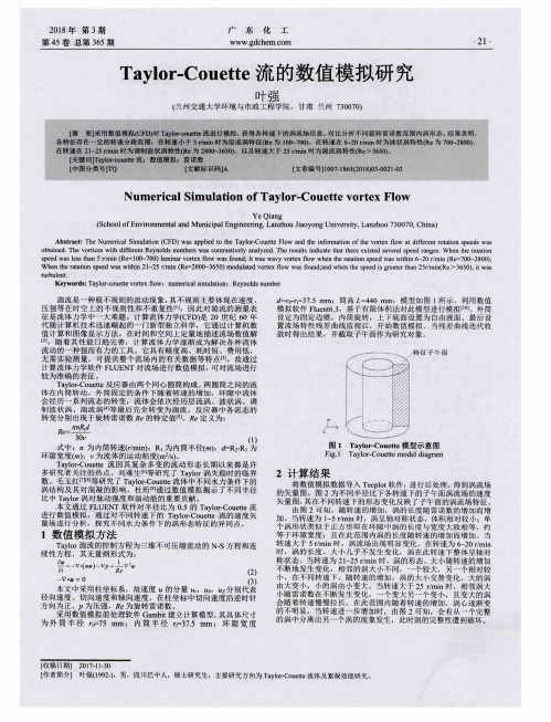
Taylor-Couette流的数值模拟研究
湍流 是 一种 极不规 则 的流动 现 象 ,其 不规 则主 要体现 在速 度 、
压 强等 在时 空 上 的不规 则性 和 不 重复 性…, 因此 对湍 流 的测 量表
1数 值 模 拟 方 法
Taylor湍流 的控 制 方程 为三 维不可 压缩 流动 的 N.S方程 和连 续性 方程 ,其无量 纲 形式 为 :
= -V.( 一 +去v 2“
一 V’Ⅳ 0
(3)
本 文 中采用 柱坐 标系 ,故 速度 “的分 量 U ,U ,U 分 别代表
径 向速 度 、切 向速度 和轴 向速度 ,在 柱坐 标 中切 向速度 沿逆 时针 方 向为 正 。P为压 强 , 为 旋转雷 诺 数 。
l,D
g l
瓣至三要
50o . 对
2s荟
啦 l392 RIr- ̄417 6 Re ̄ 97 Rt ̄ 8352 R 1113 6 P-. e= l392 3 P-.e=20 ̄ B8
Re=-2 ̄ Re=30 ̄ 4 Re ̄3340 8 R11=a176
O
Re-5568 Re= Ill
综 上所述 ,故可 将不 同水 力条 件 下 的涡形 态分 为 四个 区域 , 其转 速 范围 分别 为小 于 5 r/min、6~20 r/min、21~25 r/r ain、以及 大 于 25 r/min。
综合 对 比速度 矢量 图,与 涡对 长度 ,可 以发 现 随着 雷诺 数 的 增加 ,存 在 一定 的转 速范 围分 段 ,其 中在 同一 转速 分段 内无 论 涡 形态 还 是涡对 长度 都 具有一 定 的相似 性 ,而不 同 区段 内差别 较大 。 因此 综 合对 比分 析可 以将 其分 为 四个 区段 ,这 四个 区段 特征 分 别 符合 层流 涡 ,波 状涡 ,调制波 状 涡 以及湍 流涡特 征 。其 具体 分段 为 :当转速 为 1~5 r/min时为 波状 涡 ,转 速为 6~20 r/min时 为波状 涡 ,转速 为 21~25 r/min时 为调制 波状 涡 ,转速 大于 25 r/min为 湍 流涡 。此外 通过 对 比各特 征 线上 的切 向速 度可 以发 现切 向速 度 分 布特 征 变化 很小 ,因此 可 以得 出涡形 态特 征对 切 向速度 影 响较 小 。
fluent计算流体力学
Fluent是计算流体力学(Computational Fluid Dynamics,CFD)的一个常用软件。
CFD是用电子计算机和离散化的数值方法对流体力学问题进行数值模拟和分析的一个分支。
它结合了近代流体力学、数值数学和计算机科学,是一门具有强大生命力的边缘学科。
Fluent软件能推出多种优化的物理模型,如定常和非定常流动、层流、紊流、不可压缩和可压缩流动、传热、化学反应等。
对于每一种物理问题的流动特点,都有适合它的数值解法,用户可以选择显示或隐式差分格式,以期在计算速度、稳定性和精度等方面达到最佳。
Fluent软件之间可以方便地进行数值变换,并采用统一的前、后处理工具,这就省去了科研工作者在计算机方法、编程、前后处理等方面投入的重复、低效的劳动,而可以将主要精力和智慧用于物理问题本身的探索上。
fluent仿真计算教程
FLUENT仿真计算教程主要包含以下几个步骤:
打开FLUENT软件,选择相应的版本和求解器,然后创建新的模拟项目。
导入模型和网格文件。
在FLUENT中,可以使用Gambit或ANSYS ICEM CFD等前处理软件生成网格文件,并将其导入到FLUENT中。
在FLUENT中设置模型参数和边界条件。
例如,可以设置流体物性、流动条件(如速度、压力等)以及热力学条件等。
初始化模拟并运行模拟。
在运行模拟之前,可以设置求解器参数、迭代次数、收敛准则等。
检查模拟结果。
在模拟完成后,可以在FLUENT中查看结果,如速度场、压力场、温度场等。
同时,也可以使用后处理功能对结果进行进一步的分析和可视化。
导出模拟结果。
在FLUENT中,可以将结果导出为各种格式的文件,如ASCII、二进制等。
需要注意的是,在进行FLUENT仿真计算时,需要具备一定的流体动力学和数值计算基础,以及对所研究问题的深入理解。
同时,还需要对所使用的软件和工具进行充分的了解和熟悉。
FLUENT-6-计算模拟过程方法及步骤
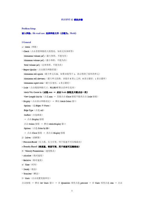
FLUENT 12 模拟步骤Problem Setup读入网格:file read case 选择网格文件(后缀为。
Mesh)1 General1)Mesh(网格)> Check(点击查看网格的大致情况,如有无负体积等)Maximum volume (m3)(最大体积,不能为负)Minimum volume (m3)(最小体积,不能为负)Total volume (m3)(总体体积,不能为负)> Report Quality(点击报告网格质量)Maximum cell squish(最大单元压扁,如果该值等于1,表示得到了很坏的单元)Maximum cell skewness(最大单元扭曲,该值在0到1之间,0表示最好,1表示最坏)Maximum aspect ratio(最大长宽比,1表示最好)> Scale(点击缩放网格尺寸,FLUENT默认的单位是米)Mesh Was Create In(点选mm →点击Scale按钮且只能点击一次)View Length Unit In(点选mm →直接点击Close按钮不能再点击Scale按钮)> Display(点击显示网格设定)→弹出Mesh Colors窗口Options(选Edges和Faces)Edge Type(点选All)Surface(点选曲面)→点击Display按钮点击Colors按钮→弹出Mesh Display窗口Options(点选Color by ID)→点击Close按钮→再点击Display按钮2)Solver(求解器)> Pressure-Based(压力基,压力可变,用于低速不可压缩流动)> Density-Based(密度基,密度可变,用于高速可压缩流动)3)Velocity Formulation(速度格式)> Absolute(绝对速度)> Relative(相对速度)4)Time(时间)> Steady(稳态)> Transient(瞬态)5)Units(点击设置变量单位)点击按钮→弹出Set Units窗口→在Quantities项里点选pressure →在Units项里点选atm →点击New按钮→点击OK按钮→点击Close按钮2 Models(物理模型)1)Multiphase(多相流模型)2)Energy(能量方程,一般要双击勾选)3)Viscous(粘性模型,一般选k-ε模型,所有参数保持默认设置)4)Radiation(辐射模型)5)Heat Exchanger(传热模型)6)Species(组分模型)7)Discrete Phase(离散相模型)8)Solidification & Melting(凝固与融化模型)9)Acoustics(声学模型,一般选择Broadband Noise Source模型,所有参数保持默认设置)3 Materials(定义材料)1)点击FLUENT Database →在FLUENT Fluid Materials里选择所需要的物质→点击Copy按钮→点击Close按钮→再点击Change/Create按钮2)点击User-Defined Database →选定写好的自定义文件→点击OK按钮3)自定义材料物性参数:在Name文本框中输入自定义材料名字gas →Chemical Formula文本框删除为空→修改Properties中各参数的值→点击Change/Create按钮→弹出Change/Create mixture and Overwrite air对话框→点击NO按钮→点击Close按钮4 Phases(相)5 Cell Zone Conditions(单元区域条件)点击Edit按钮→在Material Name项的下拉列表中选择gas(工作介质)→点击OK按钮6 Boundary Conditions(边界条件)1)Pressure-Inlet(压力进口)> Momentum(动量)Reference Frame(参考系)Gauge Total Pressure(总表压)Supersonic/Initial Gauge Pressure(初始表压或静压,一般比总表压小500Pa左右,或设为出口表压)Direction Specification Method(进口流动方向指定方法,Normal to Boundary垂直边界)Turbulence > Specification Method(湍流指定方法,Intensity and Hydraulic Diameter)Turbulent Intensity(湍流强度,一般为1)Hydraulic Diameter(水力半径,一般为管内径)> Thermal(热量)Total Temperature(总温)> Species(组分)2)Pressure -Outlet(压力出口)> Momentum(动量)Gauge Pressure(表压)Backflow Direction Specification Method(回流方向指定方法)Radial Equilibrium Pressure Distribution(径向平衡压力分布)Target Mass Flow Rate(目标质量流率)Non-Reflecting Boundary(非反射边界)Turbulence > Specification Method(湍流指定方法,点选Intensity and Hydraulic Diameter)Backflow Turbulent Intensity(回流湍流强度,一般为1)Backflow Hydraulic Diameter(回流水力半径,一般为管内径)> Thermal(热量)Backflow Total Temperature(回流总温)> Species(组分)7 Mesh Interfaces(分界面网格)8 Reference Values(参考值)9 Adapt(自适应)Adapt →Gradient(压力梯度自适应)> Options(显示选项)Refine(加密,勾选)Coarsen(粗糙,勾选)Normalize(正规化)> Method(方法)Curvature(曲率)Gradient(梯度,勾选)Iso-Value(等值)> Gradient of(梯度变量)Pressure(压力,点选)Static pressure(静压,点选)> Normalization(正常化)Standard(标准)Scale(可缩放,勾选)Normalize(使正常化)> Coarsen Threshold(粗糙比,0.3)> Refine Threshold(细化比,0.7)> Dynamic(动态)Dynamic(动态,勾选)Interval(每隔几次迭代自适应一次)→点击Mark按钮→点击Adapt按钮→(点击Compute按钮)→点击Apply按钮Solution1 Solution Methods(求解方法)1)Formulation(求解格式,默认为隐式Implicit)2)Flux Type(通量类型,默认为Roe-FDS)3)Gradient(求解格式,默认为Least Squares Cell Based)4)Flow(流动,点选二阶迎风格式Second Order Upwind)5)Turbulent Kinetic Energy(湍动能,点选二阶迎风格式Second Order Upwind)6)Turbulent Dissipation Rate(湍流耗散率,点选二阶迎风格式Second Order Upwind)2 Solution Controls1)Courant Number(库朗数,控制时间步长,瞬态计算才需要设置)2)Un-Relaxation Factors(欠松弛因子)> Turbulent Kinetic Energy(湍动能,默认为0.8)> Turbulent Dissipation Rate(湍流耗散率,默认为0.8)> Turbulent Viscosity(湍流粘度,默认为1)3)Equations(点击弹出控制方程)> Turbulence(湍流方程)> Flow(流动方程= 连续方程+ 动量方程+ 能量方程)4)Limits(点击弹出限制窗口)对某些变量使用限制值,如果计算的某个变量值小于最小限制值,则求解器就会用相应的极限取代计算值。
FLUENT喷雾模拟具体步骤

F L U E N T喷雾模拟具体
步骤
公司内部编号:(GOOD-TMMT-MMUT-UUPTY-UUYY-DTTI-
dispersion?angle?参数很重要
设置的是6?太小了
选择离散相模型DPM(拉格朗日离散粒子多相流)
Discrete Phase Model面板中的Unsteady Parameters 属性框中激活了Unsteady Tracking 选项,在瞬态流动中考虑相间耦合计算,在每一个迭代时间步长内,依据在Number Of Continuous PhaseIterations Per DPM Iteration 设定的迭代步数进行颗粒轨道的迭代计算。
液滴破碎模型:泰勒类比破碎模型
FLUENT 提供两种雾滴破碎模型:泰勒类比破碎(TAB)模型和波致破碎模型。
本文选自泰勒类比破碎模型。
Discrete Phase Model-Spray Models 下激活Droplet Breakup,TAB 模型,设置y0为0.001(初始变形值)
动态曳力模型
创建入射源:
创建喷雾模型:选择pressure-swirl-atomizer(压力旋流雾化模型)水滴颗粒相流数目:
水滴颗粒相设置:
惯性颗粒(``inert'')离散相类型(颗粒、液滴或气泡)
材料设置:
属性设置:
入射源位置
入射源轴向方向设置:流量以及时间设置:
喷嘴直径,锥角,
重力加速度设置:。
- 1、下载文档前请自行甄别文档内容的完整性,平台不提供额外的编辑、内容补充、找答案等附加服务。
- 2、"仅部分预览"的文档,不可在线预览部分如存在完整性等问题,可反馈申请退款(可完整预览的文档不适用该条件!)。
- 3、如文档侵犯您的权益,请联系客服反馈,我们会尽快为您处理(人工客服工作时间:9:00-18:30)。
Chemical Engineering Science64(2009)2941--2950Contents lists available at ScienceDirect Chemical Engineering Science journal homepage:w w w.e l s e v i e r.c o m/l o c a t e/c esOn the CFD modelling of Taylor flow in microchannels Raghvendra Gupta,David F.Fletcher∗,Brian S.HaynesSchool of Chemical and Biomolecular Engineering,The University of Sydney,Sydney,NSW,AustraliaA R T I C L E I N F O AB S T R AC TArticle history:Received22October2008Received in revised form5March2009 Accepted9March2009Available online26March2009Keywords:Taylor bubbleMicrochannelsMultiphase flowCFDMesh resolutionLiquid filmContact angle With the increasing interest in multiphase flow in microchannels and advancement in interface capturing techniques,there have recently been a number of attempts to apply computational fluid dynamics(CFD) to model Taylor flow in microchannels.The liquid film around the Taylor bubble is very thin at low Capillary number(Ca)and requires careful modelling to capture it.In this work,a methodology has been developed to model Taylor flow in microchannel using the ANSYS Fluent software package and a criterion for having a sufficiently fine mesh to capture the film is suggested.The results are shown to be in good agreement with existing correlations and previous valid modelling studies.The role played by the wall contact angle in Taylor bubble simulations is clarified.©2009Elsevier Ltd.All rights reserved.1.IntroductionWith the advancement in microfabrication techniques,the use of micro-structured devices has gained importance in a range of industrial applications.High surface-area-to-volume ratio and the small diffusion paths in such devices make them ideal candidates for heat exchangers and microreactors.The laminar nature of the flow in microchannels helps in efficient design of the micro-structured devices as no heuristic model is required to model laminar flow. Multiphase flow can further enhance the performance of these mi-crofluidic devices by providing large interfacial area(G¨unther and Jensen,2006).As a result,recently there has been an enormous inter-est in the study of two-phase adiabatic and non-adiabatic gas–liquid flow in microchannels(Suo and Griffith,1964;Barnea et al.,1983; Damianides and Westwater,1988;Barajas and Panton,1993;Fukano and Kariyasaki,1993;Mishima et al.,1993;Bao et al.,1994;Mishima and Hibiki,1996;Triplett et al.,1999;Bao et al.,2000;Zhao and Bi, 2001;Chen et al.,2002;Kawahara et al.,2002;Serizawa et al.,2002; Cubaud and Ho,2004;Pehlivan et al.,2006;Saisorn and Wongwises, 2008).Depending upon the properties and flow rates of the two flu-ids,various flow patterns such as bubbly,slug or Taylor,churn, rivulet,wavy annular,annular flow etc.occur in gas–liquid flow in microchannels.Taylor flow(also known as slug flow,Taylor bubble flow,bubble-train flow,intermittent flow,plug flow etc.)is one of the∗Corresponding author.E-mail address:d.fletcher@.au(David F.Fletcher).0009-2509/$-see front matter©2009Elsevier Ltd.All rights reserved.doi:10.1016/j.ces.2009.03.018most important flow patterns and occupies a large area on the flow-regime map(Triplett et al.,1999).Taylor flow is characterised by gas bubbles that almost fill the channel,separated by liquid slugs.A thin liquid film separates these bubbles from the wall and also connects the two successive liquid slugs separated by the gas bubble.Due to the recirculating flow in the liquid slugs,Taylor flow improves heat and mass transfer from the liquid to the wall.This flow pattern also provides a large interfacial area and thus enhances gas–liquid mass transfer.The separation of liquid slugs by the bubble also reduces axial liquid mixing.Thus,enhanced radial mass transfer and reduced axial mass transfer make Taylor flow suitable for applications which suffer from large back-mixing(Angeli and Gavriilidis,2008).Due to its interesting flow characteristics,the Taylor flow regime has received enormous attention over the years and has been stud-ied experimentally,analytically and using computational fluid dy-namics(CFD).Recently,there has been some confusion regarding the existence of the liquid film surrounding the gas bubble in various CFD modelling efforts to study Taylor flow.While some researchers acknowledge that the liquid film was not captured because a suffi-ciently refined grid was not used(Qian and Lawal,2006;Yu et al., 2007),others have carried out CFD simulations showing dry walls (no liquid film present with the gas bubble in direct contact with the wall)assuming it to be a physically acceptable result and go on to study the effect of wall contact angle on fully developed Taylor flow(He et al.,2007;Kumar et al.,2007).This work reviews the occurrence of wall dry-out during exper-imental studies and compares the observed regime with those de-scribed in numerical studies.It is shown that numerical issues,such as grid refinement,need careful attention when modelling Taylor2942R.Gupta et al./Chemical Engineering Science64(2009)2941--2950flow in microchannels and unphysical results are readily produced if sufficient care is not taken.A detailed study of the effect of various numerical practices is then presented and results are compared with widely accepted correlations.2.Literature reviewTwo-phase flow regimes in microchannels have been investi-gated experimentally by various researchers.With the exception of stratified flow,the major flow patterns that are common in macro-channels occur in microchannels,although certain flow pattern de-tails may be different from those in large channels.Fig.1shows the frequently cited flow-regime map of Triplett et al.(1999)which was developed for air–water two-phase flow in a horizontal circular channel of1.45mm inner diameter in gas superficial velocity(U GS) versus liquid superficial velocity(U LS)coordinates.Five main flow regimes were identified,as shown in Fig.1,namely bubbly,slug, churn,slug-annular and annular flow.This flow regime map is in good agreement with those reported by other researchers(Mishima and Hibiki,1996;Coleman and Garimella,1999;Yang and Shieh, 2001;Chen et al.,2002;Chung and Kawaji,2004;Pehlivan et al., 2006;Ide et al.,2007),with discrepancies generally due to a differ-ent description of the regimes.The present work is concerned with slug or Taylor flow and dry-out at the wall,and this review therefore focuses on Taylor flow and cases where wall dry-out was reported. Fig.2shows representative pictures of the slug flow pattern as observed by Triplett et al.(1999)in a1.1mm channel.This flow pattern has been referred to as slug(Suo and Griffith,1964),plug (Damianides and Westwater,1988)or bubble-train flow(Thulasidas et al.,1997).Barajas and Panton(1993)determined the flow patterns visu-ally in1.6mm horizontal channels of four different materials hav-ing different contact angles for an air–water system.Different flow patterns,such as wavy-stratified,plug,slug,annular,bubbly,rivulet etc.were observed in their experiments.Plug flow was similar to Taylor flow as defined here,while slug flow was defined as a flow pattern containing intermittent slugs of liquid blocking the entire channel cross-section.The observed flow patterns were quite simi-lar to those observed in large diameter horizontal channels(Hewitt and Hall-Taylor,1970;Coleman and Garimella,1999).Zhao and Bi(2001)investigated the air–water two-phase flow patterns in vertical equilateral triangular section channels with hy-draulic diameters of2.89,1.44and0.87mm.It was noted that,in the channel of smallest dimension,a capillary bubbly flow pattern, characterised by a train of ellipsoidal-shaped bubbles spanning al-most the entire channel cross-section,led to the side-walls being partially dry at low liquid flow rates.Serizawa et al.(2002)studied air–water two-phase flow in round tubes of20–100 m and observed different flow patterns,such as dispersed bubbly flow,gas slug flow,liquid ring flow,liquid lump flow,skewered barbecue(Yakitori)shaped flow,annular flow and rivulet flow.They also pointed out that dry and wet areas existed between the gas slug and tube wall at low velocities.Cubaud and Ho(2004)carried out experimental investigations of gas–liquid two-phase flow in200and500 m square-section mi-crochannels.In the experiments,dewetting was observed in two flow-regimes,named wedge flow and dry flow.In wedge flow they state:“For a partially wetting system,as a function of the bubble ve-locity,bubbles can dry out the center of the channel creating triple lines(liquid/gas/solid).The liquid film between the gas and the cen-ter of the channel can be considered as static,while liquid flows in the corner.”This partial dry-out of the channel walls is similar to that observed by Zhao and Bi(2001)in triangular microchannels.The dry flow occurs when the homogeneous void fraction is more than 0.995and the liquid flow is restricted to the corners of thechannel.Fig.1.Flow pattern map as observed by Triplett et al.(1999)for a1.45mm diameter circular test section.The transition lines are only indicative and are not from Triplett etal.Fig.2.Representative photograph of Taylor or slug flow in a1.1mm circular mi-crochannel as observed by Triplett et al.(1999).Taylor flow has also been studied numerically by using different approaches.Earlier studies assumed a bubble shape and simulated the flow around the bubble using a free-slip boundary condition at the bubble interface.For example,van Baten and Krishna(2004, 2005)simulated the flow in the liquid domain around the bubble and also studied mass transfer from Taylor bubbles to the liquid phase.They showed that a very fine grid(cell size smaller than 1 m for a channel of3mm diameter)was required to capture the steep concentration gradients near the bubble surface and in the liquid film.Giavedoni and Saita(1997,1999)analysed numerically the liquid flow field in the leading front and the rear part of a long bubble separately by using a finite element method which allowed the bubble interface to move.Kreutzer et al.(2005)also used a finite element method to simulate the flow around the bubble allowing the bubble interface to move.The flow of Taylor bubbles has also been studied extensively in large diameter vertical channels in the past,for example Taha and Cui(2002),Bugg and Saad(2002)and Ndinisa et al.(2005).Ndinisa et al.(2005)studied the flow of Taylor bubbles in a vertical tubular membrane of diameter19mm using different models:VOF,Eule-rian two-fluid,and a model that used a solution-adapted dispersed-phase length-scale,using ANSYS CFX-5.6.Simulations results were compared with the experimental data of Bugg and Saad(2002)and were found to be in reasonable agreement.A uniform square grid of size0.25mm was used in the simulations.It was noted that an extremely fine mesh is required to properly resolve such flows.With advances in multiphase flow modelling,various interface-capturing techniques have been used to model Taylor flow inR.Gupta et al./Chemical Engineering Science64(2009)2941--29502943microchannels:the volume-of-fluid(VOF)approach(Qian and Lawal,2006),the level-set method(Fukagata et al.,2007),or the phase-field method(He et al.,2007;He and Kasagi,2008).Com-mercial CFD codes such as ANSYS Fluent and CFD-ACE+,as well as specialised in-house codes have been used for the modelling. Commercial codes that use the VOF method,often incorporate ge-ometric reconstruction schemes(e.g.the PLIC scheme of Youngs, 1982)to capture the gas–liquid interface.Recently,Fletcher et al. (2009)reviewed CFD modelling of microchannel flows and pointed out that the main challenges in the modelling of multiphase flow in microchannels are the identification of the interface location and the occurrence of parasitic currents arising from the modelling of surface tension(Lafaurie et al.,1994;Harvie et al.,2006).Taha and Cui(2004)modelled Taylor flow in a vertical capillary for a two-dimensional,axisymmetric geometry using Fluent.A com-putational domain of length of11diameters having a grid of size 26×280was used for the simulations,with the grid being refined near the wall.The flow field was solved in a reference frame mov-ing with the bubble.A constant velocity was specified at the inlet and outflow boundary condition was used at the outlet.The results of the simulations,such as bubble velocity,diameter and velocity field around the bubble were found to be in good agreement with experimental data.Qian and Lawal(2006)used Fluent to model Taylor bubble for-mation in a T-junction microchannel for a two-dimensional planar geometry with a cross-sectional width ranging from0.25to3mm. The gas and liquid were fed from the two different legs of the T-junction.The effect of inlet configuration,gas and liquid flow rates and properties on the slug length was studied.The length of the flow domain was60tube diameters and the computational mesh contained only6600elements which is too coarse to capture the details of the flow.It was remarked,“Unfortunately,our grid reso-lution is not fine enough to capture the liquid film”.However,the results were found to be in surprisingly good agreement with the experimental data and this work is cited in numerous articles that use similarly coarse meshes.Fukagata et al.(2007)modelled two-dimensional,axisymmetric, periodic Taylor bubble flow and heat transfer(without phase change) in a20 m tube using the level-set method(Sussman et al.,1994). The void fraction,pressure gradient,bubble period and wall heat flux were used as input parameters.The bubble shape and the flow field around it were calculated and used to determine the gas and liquid superficial velocities and the two-phase frictional multiplier.They compared their results with the experimental data of Serizawa et al. (2002)and found reasonable agreement between the two.They also noticed that the bubble period has a considerable influence on the flow pattern.He et al.(2007)carried out two-dimensional axisymmetric nu-merical simulations of gas–liquid two phase flow in a channel hav-ing a radius of10 m and a length of40 m using the phase-field method.A periodic boundary condition with specified pressure drop was applied in the streamwise direction.A square grid was used with 32elements in the radial direction.Void fraction,pressure drop and initial velocity(either zero or a parabolic velocity profile)and an as-sumed bubble shape were used as the input.The final bubble shape and the superficial velocities of the gas and liquid were calculated in the simulation.The results showed that the final gas–liquid in-terface could be wall-contacting(dry)or non-wall contacting(wet) depending on the input conditions.The dry-out conditions were said to be similar to those observed in the experiments by Serizawa et al. (2002)and Cubaud and Ho(2004).However,as mentioned earlier, dry-out at the wall in the experiments of Serizawa et al.(2002)was observed at low velocities,which is not the case in the numeri-cal simulations.The dry-out mentioned by Cubaud and Ho(2004) is either typical of non-circular polygonal channels or occurs for a homogeneous void fraction greater than0.995,conditions which did not obtain in the simulations.Yu et al.(2007)studied gas–liquid flow in rectangular microchan-nels experimentally and numerically.The numerical study was car-ried out using the Lattice–Boltzmann method.The liquid film was successfully captured at capillary numbers(based on liquid prop-erties)of0.03or above.However,the film could not be captured successfully at lower values of capillary number(Ca<0.02).It was noted that this failure in capturing the liquid film could be attributed to the limited resolution of the simulations.They also pointed out,“When dry patches are formed,the flow problem becomes much more complicated,with complex moving contact lines and small droplets and bubbles sticking to the wall.This poses tremendous challenges for numerical simulation and cannot be solved by increas-ing the spatial resolution alone.”Kumar et al.(2007)studied Taylor flow numerically in curved microchannels of diameters ranging from0.25to3mm.A mesh-independence study was carried out for four different mesh densi-ties.The study showed that the gas–liquid interface became sharp as the mesh was refined,which is a direct outcome of using a re-fined mesh in the streamwise direction.However,the liquid film on the wall was not captured by even the finest mesh used,because the radial mesh was not refined sufficiently.The effect of inlet geome-try,channel diameter,curvature ratio,inlet volume fraction,surface tension,liquid viscosity and wall contact angle on slug length was studied.However,it is not possible to place any reliance on these re-sults as the hydrodynamics changes significantly with the presence of liquid film on the wall.Kashid et al.(2008)studied the hydrodynamic characteristics of liquid–liquid slug flow experimentally using the micro-PIV technique and computationally using interface capturing CFD techniques.A wall film surrounding the bubble was observed during the experi-ments.The computational studies were carried out using both the VOF and level-set methods.It was noted that the fine mesh size was one thousandth of the slug diameter.However,the wall film was not captured in the simulations.They also carried out single phase simulations by assuming the fixed interface position obtained from experimental data.Carlson et al.(2008)compared the performance of Fluent and TransAT,a high accuracy CFD code,for the simulation of multiphase flow in microchannels in the slug flow regime.The simulations in Fluent were carried out using VOF with the high order CISAM scheme used to maintain the interface sharp,while in TransAT the level-set method was used to capture the gas–liquid interface.Two-dimensional,axisymmetric simulations were carried out in a channel of1mm diameter and30mm length.The gas and liquid velocities were defined at the inlet as a uniform velocity profile.Numerical dry-out(break up of the liquid film on the tube wall,with gas in direct contact with the solid surface)was observed in the simula-tions using Fluent and the mesh near the wall needed to be refined to avoid the numerical dry-out.The bubble shape at low gas–liquid flow rates was found to be similar but the bubble frequency and the flow fields obtained from the two codes were different.At high gas–liquid flow rates,Fluent failed to capture the gas–liquid inter-face correctly.The authors pointed out that a similar deficiency in capturing the interface at a low gas–liquid flow rate was observed when the convergence criteria were relaxed.It was also observed that the choice of time integration scheme did not affect the results significantly.Lakehal et al.(2008)also used TransAT to perform a two-dimensional,axisymmetric CFD analysis of multiphase flow and heat transfer in circular horizontal miniature tube of diameter1mm, using the level-set method.The flow was modelled for a fixed liquid flow rate and different gas flow rates in the slug flow regime.By grid and domain sensitivity studies,it was shown that a channel2944R.Gupta et al./Chemical Engineering Science64(2009)2941--2950length of40diameters was required to achieve a quasi-steady state(or a fully-developed flow)for multiphase flow and around900grid elements in the axial direction were required to resolve theflow features.It was concluded that the slug flow regime in two-phase flow regime in microchannels can be modelled successfullyand qualitatively,with the flow topology captured being similar toexperimental observations.Chen et al.(2009)carried out unsteady,two-dimensional,ax-isymmetric simulations of Taylor bubble flow in a vertical channel ofdiameter1mm and length5–10mm using the level-set method.Atthe inlet,a co-flow nozzle arrangement(including nozzle wasused to inject air and octane.The fully developed circular and annularchannel velocity profiles were specified for the gas and liquid,respec-tively.At the nozzle wall,no penetration and the Navier-slip condi-tions(u slip=− (*u/*y)wall,where is the slip length)were specified for the normal and tangential velocity components,respectively.Atthe outlet,either outflow or a fully developed velocity profile with amean velocity equal to inlet two-phase velocity was specified.Bothof the outlet boundary conditions gave similar results until the bub-ble reached the outlet.A contact line model was applied to considerthe effect of hysteresis and the dynamic nature of the contact angleat the nozzle wall.The grid spacing used in the simulation was1/60th of the channel diameter.The results were compared withthe experimental data of Salman et al.(2006)and found to be ingood agreement.It was noted that the formation of Taylor bubbleswas mainly dependent on the relative magnitudes of the gas andliquid superficial velocities for a given nozzle/tube configuration.However,a change in nozzle geometry could change the size ofthe Taylor bubbles and pressure drop significantly for the samesuperficial velocities.Fang et al.(2008)studied the evolution of liquid slug flow withsidewall liquid injection in rectangular microchannels experimen-tally and numerically.A model was proposed to include the walladhesion forces by considering the effect of contact angle hysteresisand it was demonstrated that the model including hysteresis effectpredicted the liquid slug detachment in excellent agreement withthose measured in the experiments.It was also shown that the re-sults were quite different when a constant contact angle was usedin the model.This study shows that the effect of dynamic contactangle needs to be modelled accurately to capture the slug growthand detachment behaviour at the wall in the injector region.Liu and Wang(2008)investigated upward Taylor flow in verticalsquare and equilateral triangular capillaries of hydraulic diameter1mm and length16mm using Fluent.A fully developed velocity pro-file was set at the inlet and an outflow boundary condition was usedat the outlet.The simulations were carried out in a reference framemoving with the bubble.The liquid inlet velocity was iteratively ad-justed until the position and shape of the bubble were stable in thedomain.The bubble size and shape,film thickness and velocity fieldwere studied as a function of Capillary number.Although not directly related to Taylor bubbles,the numericalstudy of droplet behaviour in a sudden contraction by Rosengartenet al.(2006)highlights the role the contact angle can play whenthe film surrounding the“bubble”becomes very thin and can beinfluenced by long range van der Waal forces.Both experimentaland computational results are used to illustrate the effect of contactangle for very thin films.The above review of the literature on two-phase gas–liquid flowin microchannels shows that:•Taylor bubble flow has been observed as an important flow regime in the experimental studies to establish flow-regime maps of gas–liquid flow in microchannels.•The bubbles are almost always surrounded by the liquid.Dry-out at the wall has been observed under only very particular condi-tions,such as non-circular geometries or very high homogeneous void fraction( >0.995).This dry-out on the wall is a three-dimensional phenomenon and requires the use of three dimen-sional modelling that includes a dynamic contact angle model.•Numerous numerical studies have been carried out to model Tay-lor flow in microchannels.The liquid film at the wall has not been captured successfully in many of these studies due to poor reso-lution of the flow near the wall.This deficiency of the numerical simulation has a profound effect on frictional pressure drop and heat and mass transfer to the wall.Capturing the liquid film is crucial in the numerical modelling of Taylor flow.•Some researchers believe that the wall adhesion properties,such as wall contact angle,play an important role in Taylor flow modelling. This is not entirely true.The role of the wall contact angle is only important when both of the fluids are in contact with the wall or the film is so thin that van der Waal forces can act across the film. This may be the case in T or Y type junctions where both phases remain in contact with the wall but once a Taylor bubble flow is obtained with a liquid film at the wall,wall adhesion plays no role in determining the bubble shape.Moreover,the modelling of wall adhesion requires inclusion of the contact angle hysteresis effect to obtain meaningful results.3.Mathematical modellingThe usual approach to the modelling of multiphase flow in mi-crochannels is to compute the evolution of the gas–liquid interface (Hessel et al.,2004).This can be achieved by using a“single-fluid”formulation in which a common flow field is shared by all of the phases.The hydrodynamics of such flows can be described by the equations for the conservation of mass and momentum,together with an additional advection equation to determine the gas–liquid interface.For an incompressible,Newtonian fluid,these equations can be written as follows:Continuity:**t+∇.V=0(1) Momentum:*( V)t+∇.( V⊗V)=−∇p+∇.( (∇V+∇V T))+F s(2) Volume fraction:*t+V.∇ =0(3)where V denotes the velocity vector,p the pressure, the density and the dynamic viscosity of the fluid.F s is the surface tension force approximated as a body force in the vicinity of the interface,and is the volume fraction of one of the phases.The bulk properties,such as density and viscosity,are determined from the volume-fraction weighted average of the properties of the two fluids.In the present work,the flow field has been calculated using a two-dimensional,axisymmetric(cylindrical)geometry in order to save computational time and effort.The effect of gravity has been neglected as it plays a minor role in multiphase flow in microchan-nels(Triplett et al.,1999).Fig.3shows a schematic of the channel and the boundary conditions applied.At the inlet,the gas enters at the core and the liquid enters as an annulus around the gas core.Plug flow of the gas and the liquid is assumed.At the outlet,a constant area-averaged pressure boundary condition is applied.The usual no-slip boundary condition is applied at the wall and a zero nor-mal gradient boundary condition for all the variables is applied on the axis.R.Gupta et al./Chemical Engineering Science64(2009)2941--29502945Fig.3.Schematic representation of the geometry and boundary conditions used in the simulations.4.Solution methodologyThe Fluent commercial CFD software is used to model two-dimensional,axisymmetric,transient,two-phase Taylor flow in a microchannel.This section describes the details of various numerical schemes used.4.1.VOF MethodThe volume-of-fluid method(Hirt and Nichols,1981)is used to identify the gas–liquid interface by solving a volume fraction equa-tion(Eq.(3)above)for one of the phases.An explicit geometric re-construction scheme is used to represent the interface by using a piecewise-linear approach(Youngs,1982).The time step used for the VOF equation in Fluent is not necessarily the same as that used for the other equations but is calculated based upon the character-istic transit time of a fluid element across a control volume and is limited by a specified maximum value for the Courant number.The time taken to empty a cell is calculated by dividing the volume of each cell by the sum of the outgoing fluxes in the region near the fluid interface.The smallest such time is used as the characteris-tic time of transit for a fluid element across a control volume.The Courant number(Co)is defined by Eq.(4)asCo=tfluid(4)where x is the grid size and V fluid is the fluid velocity.A maximum Courant number of0.25is set in the present calculations and a vari-able time step based on a fixed Courant number of0.25or less was used to force the time step to be the same for all the equations. 4.2.Surface tension modelThe continuum surface force(CSF)model proposed by Brackbill et al.(1992)is used to model surface tension effects.The CSF model approximates the surface tension-induced stress by a body force, which acts throughout a small but finite fluid region surrounding the interface.The surface tension force per unit area is represented asF s= (r−r int)n(5) where is the coefficient of surface tension,j is the radius of curva-ture, (r)is the Dirac delta function and n denotes the unit normal vector on the interface.The normal n and curvature j in Eq.(5)are defined in terms of the volume fraction( )via:n=∇|∇ |(6)and=∇.n(7)This implementation of the surface tension force can induce unphys-ical velocity near the interface known as`spurious currents'(Lafaurie et al.,1994;Harvie et al.,2006).This occurs because the pressure and viscous force terms do not exactly balance the surface tension-1500-900-3003009001500Pressure (Pa)Cell-based gradientsNode-based gradientsFig.4.Pressure distribution after∼7.1ms for(a)Green–Gauss node-based gradients (b)Green–Gauss cell-based gradients for a100×2000mesh and U LS=0.255m/s andU GS=0.245m/s.The simulations for the two cases were started using the same initial conditions.The bubble interface is shown by a black line.force.The accurate calculation of gradients can help in minimising these spurious currents.A contact angle of90◦was specified in all cases.In Fluent the contact angle is used to adjust the surface normal in cells near the wall and therefore sets the curvature of the interface near the wall. Given that there is no gas–solid–liquid interface present at the inlet or when Taylor bubbles are present this model should not have any effect on the results.However,as we will see later it determines the “bubble”shape in poorly resolved simulations.In Fluent the gradient of scalars(pressure,velocity components and volume fraction)must be calculated at the cell centre from the scalar values at the cell face centroids.Two different meth-ods,namely Green–Gauss cell-based and Green–Gauss node-based, are available to calculate the cell face centroid values of scalars for structured meshes.In cell-based calculations,the cell face centroid values are computed from the arithmetic average of the values at the neighbouring cell centres,whilst in node-based calculations,cell face centroid values are computed by the arithmetic average of the nodal values on the faces.The nodal values are computed from the weighted average of the cell values surrounding the nodes.It is worth emphasising here that the gradients are computed at the cell centres for both cell-based and node-based gradient calculations. Fig.4shows the pressure contour around a bubble for calculations using the Green–Gauss cell-based and node-based gradient methods. Both the cases were run using the same discretization and numeri-cal schemes and were started using the same initial condition.In the cell-based gradient case,significant unphysical pressure oscillations are observed in the liquid film near the bubble interface.These re-sult in a very erratic velocity field in the film.It is evident from the figure that using node-based gradients helps to minimise these un-physical oscillations,although small unphysical pressure oscillation still remain at the head and tail of the bubble.4.3.Solver optionsAn implicit body force treatment(for the surface tension force in the present case)is used to take into account the partial equilib-rium of the pressure gradient and body forces,as recommended in Fluent6.3.26Users'Guide(2006).Fluent uses a co-located scheme in which pressure and velocity are stored at the cell centres.However, the calculation of pressure gradients requires the pressure values to be interpolated from cell centres to the cell faces.In the present computations,a body-force-weighted interpolation scheme is used。