An efficient joint source-channel coding for a D-dimensional array
央财金融硕士考研—金融学院

中央财经大学——金融学院“考金融,选凯程”!凯程2014中财金融硕士保录班录取8人,专业课考点全部命中,凯程在金融硕士方面具有独到优势,全日制封闭式高三集训,并且在金融硕士方面有独家讲义\独家课程\独家师资\独家复试资源,确保学生录取.其中8人中有4人是二本学生,1人是三本学生,3人是一本学生,金融硕士只要进行远程+集训,一定可以取得成功.摘要现任中央财经大学金融学院教授、院长、院学术委员会主任、国际金融研究中心主任。
毕业于中国人民大学经济学院,获经济学博士。
享受国务院政府特殊津贴,入选“新世纪百千万人才工程(国家级)”、教育部“新世纪优秀人才支持计划”、财政部“跨世纪学科带头人”。
曾在荷兰蒂尔堡大学、世界银行学院、美国国际经济研究所、哥伦比亚大学地球研究院、澳大利亚国立大学做高级访问学者。
兼任中国世界经济学会副会长、中国国际金融学会常务理事及副秘书长、中国国际经济关系学会常务理事、中国金融学会理事、中国财经教育分会金融专业协作组主任委员、亚太经济与金融论坛主席、亚洲经济专家会议(Asian Economic Panel,New York/Tokyo/Seoul)成员、中国证监会第12届发审会委员、中国人民银行货币政策委员会专家咨询组成员、X 鸿儒金融教育基金会学术委员、中国人民银行研究生部学位委员。
研究领域为国际金融和宏观经济。
曾主持国家自然科学基金项目、国家社会科学基金项目、教育部人文社科项目等课题,研究内容涉及新兴市场经济体的资本账户开放、金融自由化、全球经济失衡、国际货币体系改革、经济全球化、汇率制度和货币国际化等。
在《经济研究》、《世界经济》、《金融研究》和《国际金融研究》等学术刊物发表论文80余篇,出版学术著作10余本(包括主编和合著)。
近年来,作为亚洲经济专家会议(AEP)成员、亚欧经济论坛(AEEF)成员、德国开发研究院(GDI)中国地区协调人等,曾赴美国、英国、德国、意大利、挪威、日本、韩国、泰国、越南、印度尼西亚、马来西亚、新加坡、澳大利亚、巴西、XX和XX等国家和地区参加国际学术会议或进行公开演讲。
均相合成多重选择性的新型两亲性C22高效液相色谱固定相

第42 卷第 12 期2023 年12 月Vol.42 No.121580~1587分析测试学报FENXI CESHI XUEBAO(Journal of Instrumental Analysis)均相合成多重选择性的新型两亲性C22高效液相色谱固定相范二乐1,蒋星宇1,张加栋1*,张明亮2,韩海峰1,2,张大兵1,2,陈义1,3(1.淮阴工学院矿盐资源深度利用技术国家地方联合工程研究中心,高端矿盐功能材料智能制备国际合作联合实验室,江苏淮安223003;2.江苏汉邦科技股份有限公司,江苏淮安223000;3.中国科学院化学研究所活体分析化学科学院重点实验室,北京100190)摘要:为解决高效液相色谱(HPLC)固定相非均相合成中产物多变和重现性差等问题,该文采用均相合成新方法,制备了既含有二十二碳烷基(C22)、又嵌入脲(U)和/或酰胺(A)强极性基团的两种新型两亲性色谱固定相C22-A和C22-A/U。
通过元素分析、核磁等手段,证实制备的两种新型固定相含有碳、氮元素,且碳氮元素比例符合理论值,表明酰胺和脲基极性基团成功键合到硅胶上。
通过对多种样品进行色谱分离分析,对两种新型固定相的载体残余硅羟基屏蔽作用、疏水选择性、形状选择性和亲水性等多种性质进行了考察,证实两种新型固定相不但具备作为反相液相色谱(RPLC)的性能,同时也具备亲水相互作用色谱(HILIC)的性能。
相较于C18固定相,C22-A和C22-A/U具有更好的形状选择性,双重嵌入的极性基团极大地降低了固定相硅羟基活性。
将C22-A和C22-A/U两种固定相应用于几种碱性化合物、雌醇(酮)类化合物的分离,C22固定相在一定程度上解决了传统C18固定相上碱性化合物分离拖尾严重或保留不足的问题,成功实现了对雌醇(酮)类化合物的分离。
关键词:色谱固定相;两亲性;均相合成;药物分析;液相色谱中图分类号:O657.7;R914.1文献标识码:A 文章编号:1004-4957(2023)12-1580-08 Homogeneous Synthesis of Novel Amphiphilic C22 StationaryPhases with Multiple SelectivityFAN Er-le1,JIANG Xing-yu1,ZHANG Jia-dong1*,ZHANG Ming-liang2,HAN Hai-feng1,2,ZHANG Da-bing1,2,CHEN Yi1,3(1.International Cooperation Joint Laboratory for Intelligent Preparation of High-end Functional Mineral SaltMaterials,National & Local Joint Engineering Research Center for Mineral Salt Deep Utilization,Huaiyin Instituteof Technology,Huai’an 223003,China;2.Jiangsu Hanbon Science & Technology Co.Ltd.,Huai’an 223000,China;3.CAS Key Laboratory of Analytical Chemistry for Living Biosystems,Instituteof Chemistry,Chinese Academy of Sciences,Beijing 100190,China)Abstract:In order to solve the variable and irreproducible issues of heterogeneously synthesized chromatographic stationary phases,a new method of homogeneous synthesis was established and used to prepare two newly designed amphiphilic stationary phases,C22-A and C22-A/U,where C22 denotes a long docosyl terminal while U and A denote the strong polar insertions of urea and am⁃ide groups at the initial end,respectively. By the means of elemental analysis and nuclear magnetic spectrum,the two new stationary phases contain nitrogen elements,and the ratio of carbon and nitro⁃gen elements accords with the theoretical value,indicating that the amide and urea-based polar groups are successfully bonded to silica gel. Through the chromatographic separation and analysis of the standard sample and the real sample,the shielding effect on upported silicon hydroxyl,hydro⁃phobic selectivity,shape selectivity and hydrophilicity of the two new stationary phases were investi⁃gated.It is confirmed that the two new stationary phases have amphiphilic properties as reversed-phase liquid chromatography(RPLC)and hydrophilic interaction chromatography(HILIC).Com⁃pared with C18 stationary phases,C22-A and C22-A/U own better shape selectivity,and the dou⁃doi:10.19969/j.fxcsxb.23072402收稿日期:2023-07-24;修回日期:2023-09-15基金项目:国家自然科学基金重点项目(22134007)∗通讯作者:张加栋,博士,副教授,研究方向:化学与生物传感、色谱分离分析等,E-mail:jiadongzhang@1581第 12 期范二乐等:均相合成多重选择性的新型两亲性C22高效液相色谱固定相ble embedded polar groups greatly reduce the silica hydroxyl activity of the stationary phase. C22-A and C22-A/U were used for the separation of several alkaline compounds and estrone(ketone) com⁃pounds. The C22 stationary phase solved the problem of serious tailing or insufficient retention of al⁃kaline compounds in the traditional C18 alkyl stationary phase,and successfully realized the separa⁃tion of estrone(ketone) compounds.Key words:chromatographic stationary phase;amphiphilicity;homogeneous synthesis;drug analysis;liquid chromatography色谱固定相的性质决定了保留机理、分离效率以及适合的分离对象[1-2]。
the hydrogen bond in the solid state
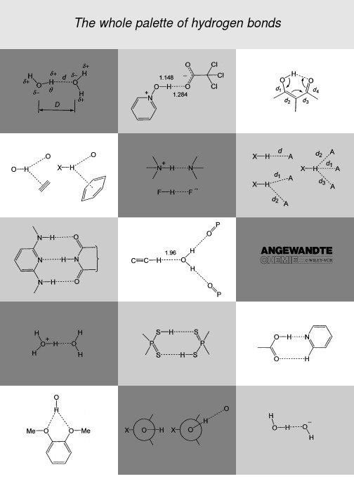
1.IntroductionThe hydrogen bond was discovered almost 100years ago,[1]but still is a topic of vital scientific research.The reason forthis long-lasting interest lies in the eminent importance ofhydrogen bonds for the structure,function,and dynamics of avast number of chemical systems,which range from inorganicto biological chemistry.The scientific branches involved arevery diverse,and one may include mineralogy,materialscience,general inorganic and organic chemistry,supramo-lecular chemistry,biochemistry,molecular medicine,andpharmacy.The ongoing developments in all these fields keepresearch into hydrogen bonds developing in parallel.In recentyears in particular,hydrogen-bond research has stronglyexpanded in depth as well as in breadth,new concepts havebeen established,and the complexity of the phenomenaconsidered has increased dramatically.This review is intendedto give a coherent survey of the state of the art,with a focus onthe structure in the solid state,and with weight put mainly on the fundamental aspects.Numerous books [2±9]and reviews on the subject have appeared earlier,so a historical outline is not necessary.Much of the published numerical material is somewhat outdated and,therefore,this review contains some numerical data that have been newly retrieved from the most relevant structural database,the Cambridge Structural Data-base (CSD).[10]It is pertinent to recall here the earlier ™classical∫view on hydrogen bonding.One may consider the directional inter-action between water molecules as the prototype of all hydrogen bonds (Scheme 1,definitions of geometric parameters are also in-cluded).The large difference in electro-negativity between the H and O atoms makes the O ÀH bonds of a water molecule inherently polar,with partial atomic charges of around 0.4on each H atom and À0.8on the O atom.Neighboring water molecules orient in such a way that local dipoles O d ÀÀH d point at negative partial charges O d À,that is,at the electron lone pairs of the filled p orbitals.In the resulting The Hydrogen Bond in the Solid StateThomas Steiner*In memory of JanKroon[*]Dr.T.SteinerInstitut f¸r Chemie–KristallographieFreie Universit‰t BerlinTakustrasse 6,14195Berlin (Germany)Fax:( 49)30-838-56702E-mail:steiner@chemie.fu-berlin.deREVIEWSREVIEWS T.SteinerOÀH¥¥¥j O interaction,the intermolecular distance is short-ened by around1äcompared to the sum of the van der Waals radii for the H and O atoms[11](1ä 100pm),which indicates there is substantial overlap of electron orbitals to form a three-center four-electron bond.Despite significant charge transfer in the hydrogen bond,the total interaction is dominantly electrostatic,which leads to pronounced flexibil-ity in the bond length and angle.The dissociation energy is around3±5kcal molÀ1.This brief outline of the hydrogen bond between water molecules can be extended,with only minor modifications,to analogous interactions XÀH¥¥¥A formed by strongly polar groups X dÀÀH d on one side,and atoms A dÀon the other (X O,N,halogen;A O,N,S,halide,etc.).Many aspects of hydrogen bonds in structural chemistry and structural biology can be readily explained at this level,and it is certainly the relative success of these views that made them dominate the perception of the hydrogen bond for decades.This dominance has been so strong in some periods that research on hydrogen bonds differing too much from the one between water molecules was effectively impeded.[8]Today,it is known that the hydrogen bond is a much broader phenomenon than sketched above.What can be called the™classical hydrogen bond∫is just one among many–a very abundant and important one,though.We know of hydrogen bonds that are so strong that they resemble covalent bonds in most of their properties,and we know of others that are so weak that they can hardly be distinguished from van der Waals interactions.In fact,the phenomenon has continuous transition regions to such different effects as the covalent bond,the purely ionic,the cation±p,and the van der Waals interaction.The electrostatic dominance of the hydrogen bond is true only for some of the occurring configurations,whereas for others it is not.The H¥¥¥A distance is not in all hydrogen bonds shorter than the sum of the van der Waals radii.For an XÀH group to be able to form hydrogen bonds,X does not need to be™very electroneg-ative∫,it is only necessary that XÀH is at least slightly polar. This requirement includes groups such as CÀH,PÀH,and some metal hydrides.XÀH groups of reverse polarity, X d ÀH dÀ,can form directional interactions that parallel hydrogen bonds(but one can argue that they should not be called so).Also,the counterpart A does not need to be a particularly electronegative atom or an anion,but only has to supply a sterically accessible concentration of negative charge. The energy range for dissociation of hydrogen bonds covers more than two factors of ten,about0.2to40kcal molÀ1,and the possible functions of a particular type of hydrogen bond depend on its location on this scale.These issues shall all be discussed in the following sections.For space reasons,it will not be possible to cover all aspects of hydrogen bonding equally well.Therefore,some important fields,for which recent guiding reviews are available,will not be discussed in great length.One example is the role of hydrogen bonds in molecular recognition patters(™supra-molecular synthons∫),[12]and the use of suitably robust motifs for the construction of crystalline archtitectures with desired properties(™crystal engineering∫).[13,14]This area includes the interplay of hydrogen bonds with other intermolecular forces, with whole arrays of such forces,and hierarchies within such an interplay.The reader interested in this complexfield is referred to the articles of Desiraju,[12,13]Leiserowitz et al.,[15] and others.[16]A further topic which could not be covered here is the symbolic description of hydrogen bond networks using tools of graph theory,[17]in particular the™graph set analy-sis∫.[18]An excellent guiding review is also available in this case.[19]For hydrogen bonding in biological structures,the interested reader is referred to the book of Jeffrey and Saenger,[5]and for theoretical aspects to the book of Scheiner[7]as well as other recent reviews.[20]Results obtained with experimental methods other than diffraction will be touched upon only briefly,and will possibly leave some readers dissatisfied.The role of hydrogen bonding in special systems will not be discussed at all,simply because there are too many of them.2.Fundamentals2.1.Definition of the Hydrogen BondBefore discussing the hydrogen bond itself,the matter of hydrogen bond definitions must be addressed.This is an important point,because definitions of terms often limit entire fields.It is,also,a problematic point because very different hydrogen bond definitions have been made,and partREVIEWS Solid-State Hydrogen Bondsof the literature relies quite uncritically on the validity(or thevalue)of the particular definition that is adhered to.Time has shown that only very general and flexibledefinitions of the term™hydrogen bond∫can do justice tothe complexity and chemical variability of the observedphenomena,and include the strongest as well as the weakestspecies of the family,and inter-as well as intramolecularinteractions.A far-sighted early definition is that of Pimenteland McClellan,who essentially wrote that™...a hydrogenbond exists if1)there is evidence of a bond,and2)there isevidence that this bond sterically involves a hydrogen atomalready bonded to another atom∫.[2]This definition leaves thechemical nature of the participants,including their polaritiesand net charges,unspecified.No restriction is made on theinteraction geometry except that the hydrogen atom must besomehow™involved∫.The crucial requirement is the existenceof a™bond∫,which is itself not easy to define.The methods totest experimentally if requirements1and2are fulfilled arelimited.For crystalline compounds,it is easy to see withdiffraction experiments whether an H atom is involved,but itis difficult to guarantee that a given contact is actually™bonding∫.A drawback of the Pimentel and McClellan definition isthat in the strict sense it includes pure van der Waals contacts(which can be clearly™bonding∫,with energies of severaltenths of a kcal molÀ1),and it also includes three-center two-electron interactions where electrons of an XÀH bond are donated sideways to an electron-deficient center(™agosticinteraction∫).From a modern viewpoint,it seems advisable tomodify point2,such as by requiring that XÀH acts as a proton (not electron)donor.Therefore,the following definition is proposed:An XÀH¥¥¥A interaction is called a™hydrogen bond∫,if 1.it constitutes a local bond,and2.XÀH acts as proton donor to A.The second requirement is related to the acid/base proper-ties of XÀH and A,and has the chemical implication that a hydrogen bond can at least in principle be understood as an incipient proton-transfer reaction from XÀH to A.It excludes, for example,pure van der Waals contacts,agostic interactions, so-called™inverse hydrogen bonds∫(see Section8),and B-H-B bridges.As a matter of fact,point2should be interpreted liberally enough to include symmetric hydrogen bonds XÀHÀX,where donor and acceptor cannot be distin-guished.The direction of formal or real electron transfer in a hydrogen bond is reverse to the direction of proton donation.Apart from general chemical definitions,there are manyspecialized definitions of hydrogen bonds that are based oncertain sets of properties that can be studied with a particulartechnique.For example,hydrogen bonds have been definedon the basis of interaction geometries in crystal structures(short distances,fairly™linear angles∫q),certain effects in IRabsorption spectra(red-shift and intensification of n XH,etc.),or certain properties of experimental electron density distri-butions(existence of a™bond critical point∫between H andA,with numerical parameters within certain ranges).All suchdefinitions are closely tied to a specific technique,and may be quite useful in the regime accessible to it.Nevertheless,theyare more or less useless outside that regime,and many amisunderstanding in the hydrogen bond literature has beencaused by applying such definitions outside their region ofapplicability.The practical scientist often requires a technical definition,and automated data treatment procedures for identifyinghydrogen bonds cannot be done without.It is not within thescope of this article to discuss any set of threshold values thata™hydrogen bond∫must pass in any particular type oftechnical definition.It is only mentioned that the™van derWaals cutoff∫definition[21]for identifying hydrogen bonds ona structural basis(requiring that the H¥¥¥A distance issubstantially shorter than the sum of the van der Waals radiiof H and A)is far too restrictive and should no longer beapplied.[5,6,8]If distance cutoff limits must be used,XÀH¥¥¥A interactions with H¥¥¥A distances up to3.0or even3.2äshould be considered as potentially hydrogen bonding.[6]Anangular cutoff can be set at>908or,somewhat moreconservatively,at>1108.A necessary geometric criterionfor hydrogen bonding is a positive directionality preference,that is,linear XÀH¥¥¥A angles must be statistically favored over bent ones(this is a consequence of point2of the above definition).[22]2.2.Further TerminologyA large part of the terminology concerning hydrogen bonds is not uniformly used in the literature,and still today, terminological discrepancies lead to misunderstanding be-tween different authors.Therefore,some of the technical terms used in this review need to be explicitly defined.In a hydrogen bond XÀH¥¥¥A,the group XÀH is called the donor and A is called the acceptor(short for™proton donor∫and™proton acceptor∫,respectively).Some authors prefer the reverse nomenclature(XÀH electron acceptor,Y electron donor),which is equally justified.In a simple hydrogen bond,thedonor interacts with one acceptor(Scheme2a).Since the hydro-gen bond has a long range,adonor can interact with two andthree acceptors simultaneously(Scheme2b,c).Hydrogen bondswith more than three acceptorsare possible in principle,but areonly rarely found in practice be-cause they require very highspatial densities of acceptors.The terms™bifurcated∫and™tri-furcated∫are commonly used todescribe the arrangements inScheme2b and c,respectively.The term™two-centered∫hydro-gen bond is an alternative descrip-tor for XÀH¥¥¥A(Scheme2a)where the H-atom is bonded totwo other atoms,and is itself notX H AX HAX H AAAAb)c)a)dd1d2d1d2d3Scheme2.Different typesof hydrogen bridges.a)Nor-mal hydrogen bond with oneacceptor.b)Bifurcated hy-drogen bond;if the twoH¥¥¥A separations are dis-tinctly different,the shorterinteraction is called majorcomponent,and the longerone the minor component ofthe bifurcated bond.c)Tri-furcated hydrogen bond.REVIEWST.Steiner counted as a center.Consequently,the arrangements in Scheme 2b and 2c may be called ™three-∫and ™four-centered∫hydrogen bonds,respectively.[5,6]This terminology is logical,but leads to confusion from the point of view of regarding hydrogen bonds O ÀH ¥¥¥O as ™three-center four-electron∫interactions,where the H-atom is counted as a center.A bifurcated hydrogen bond (Scheme 2b)is then termed ™three-centered∫,but also represents a ™four-center six-electron∫interaction.To avoid such ambiguities,the older term ™bifurcated∫is used here.There is particular confusion concerning the terms attrac-tive and repulsive .Some authors use these terms to character-ize forces,and others to characterize energies.In the latter case,an ™attractive interaction∫is taken as a synonym for ™bonding interaction∫,that is,one that requires the input of energy to be broken.Following well-founded recommenda-tions,[23]the terms ™attractive∫and ™repulsive∫are used here exclusively to describe forces.Negative and positive bond energies are indicated by the terms ™stabilizing∫(or ™bond-ing∫)and ™destabilizing∫,respectively.The schematic hydro-gen bond potential in Figure 1shows that a stabilizing interaction (that is,with E <0)is associated with a repulsive force if it is shorter than the equilibrium distance (see figure legend for further details).[8]Figure 1.Schematic representation of a typical hydrogen bond potential.[8]A hydrogen bond length differing from d 0implies a force towards a geometry of lower energy,that is,by attraction if d >d 0and repulsion if d <d 0.Note that the interaction can at the same time be ™stabilizing∫(or ™bonding∫)and ™repulsive∫!The distortions from d 0occurring in practice are limited by the energy penalties that have to be paid,and in crystals,only a few hydrogen bonds have energies differing by more than 1kcal mol À1from optimum.Hydrogen bonds are sometimes called ™nonbonded inter-actions∫.At least to this author,this appears a contradiction in terms which should be avoided.2.3.Constituent InteractionsThe hydrogen bond is a complexinteraction composed of several constituents that are different in their natures.[6,7]Most popular are partitioning modes that essentially follow those used by Morokuma.[24]The total energy of a hydrogen bond (E tot )is split into contributions from electrostatics (E el ),polarization (E pol ),charge transfer (E ct ),dispersion (E disp ),and exchange repulsion (E er ),somewhat different,but still related,partitioning schemes are also in use.The distance and angular characteristics of these constituents are very different.The electrostatic term is directional and of long range (diminishing only slowly as Àr À3for dipole ±dipole and as Àr À2for dipole ±monopole interactions).Polarization de-creases faster (Àr À4)and the charge-transfer term decreases even faster,approximately following e Àr .According to natural bond orbital analysis,[25]charge transfer occurs from an electron lone pair of A to an antibonding orbital of X ÀH,that is n A 3s *XH .The dispersion term is isotropic with a distance dependence of Àr À6.The exchange repulsion term increases sharply with reducing distance (as r À12).The dispersion and exchange repulsion terms are often combined into an isotropic ™van der Waals∫contribution that is approx-imately described by the well-known Lennard ±Jones poten-tial (E vdW $A r À12ÀB r À6).Depending on the particular chem-ical donor ±acceptor combination,and the details of the contact geometry,all these terms contribute with different weights.It cannot be globally stated that the hydrogen bond as such is dominated by this or that term in any case.Some general conclusions can be drawn from the overall distance characteristics.In particular,it is important that of all the constituents,the electrostatic contribution reduces slowest with increasing distance.The hydrogen bond potential for any particular donor ±acceptor combination (Figure 1)is,there-fore,dominated by electrostatics at long distances,even if charge transfer plays an important role at optimal geometry.Elongation of a hydrogen bond from optimal geometry always makes it more electrostatic in nature.In ™normal∫hydrogen bonds E el is the largest term,but a certain charge-transfer contribution is also present.The van der Waals terms too are always present,and for the weakest kinds of hydrogen bonds dispersion may contribute as much as electrostatics to the total bond energy.Purely ™electrostatic plus van der Waals∫models can be quite successful despite their simplicity for hydrogen bonds of weak to intermediate strengths.[26]Such simple models fail for the strongest types of hydrogen bonds,for which their quasi-covalent nature has to be fully considered (see Section 7).2.4.Energies The energy of hydrogen bonds in the solid state cannot be directly measured,and this circumstance leaves open ques-tions in many structural putational chemistry,on the other hand,produces results on hydrogen bond energies at an inflationary rate,[7,20]many obtained at high levels of theory and even more in rather routine calculations using black-box methods.Theoretical studies are not the topic of the present review,but an idea of typical results can be gained from the collection of calculated values listed in Table 1.[27]It appears that hydrogen bond energies cover more than two orders of magnitude,about À0.2to À40kcal mol À1.On a logarithmic scale,the bond energy of the water dimer is roughly in the middle.REVIEWS Solid-State Hydrogen BondsThe values in Table1are computed for dimers in optimal geometry undisturbed by their surroundings.In the solid state, hydrogen bonds are practically never in optimal geometry, and are always influenced by their environment.There are numerous effects from the close and also from the remote surrounding that may considerably increase or lower hydro-gen bond energies(™crystal-field effects∫).Hydrogen bonds do not normally occur as isolated entities but form networks. Within these networks,hydrogen bond energies are not additive(see Section4).In such cases,it is not reasonable to split up the network into individual hydrogen bonds and to calculate energies for each one.In this sense,calculated hydrogen bond energies should always be taken with caution.2.5.Transition to Other Interaction TypesAs outlined previously,the hydrogen bond is composed of several constituent interactions which are variant in their contributing weights.Chemical variation of donor and/or acceptor,and possibly also of the environment,can gradually change a hydrogen bond to another interaction type.This shall be detailed here for the most important cases.The transition to pure van der Waals interaction is very common.The polarity of XÀH or A(or both)in the array X dÀÀH d ¥¥¥A dÀcan be reduced by suitable variation of X or A.This reduces the electrostatic part of the interaction, whereas the van der Waals component is much less affected. In consequence,the van der Waals component gains relative weight,and the angular characteristics gradually change from directional to isotropic.Since the polarities of X dÀÀH d or A dÀcan be reduced to zero continuously,the resulting transition of the interaction from hydrogen bond to van der Waals type is continuous too.Such a behavior was actually demonstrated for the directionality of CÀH¥¥¥O C interactions,which gradually disappears when the donor is varied from C CÀH to C CH2to CÀCH3(see Figure8,Section3.2).[22]At the acceptor side of a hydrogen bond,sulfur is typical of an atom that allows continuous variation of the partial charge from S dÀto S d .Therefore,one can create a continuum of chemical situations between the S atom acting as a fairly strong hydrogen bond acceptor,and being inert to hydrogen bonding (the extreme cases are ionic species such as XÀSÀand X S ÀY).At the other end of the energy scale,there is a continuous transition to covalent bonding.[28]In the so-called symmetric hydrogen bonds XÀHÀX,where an H atom is equally shared between two chemically identical atoms X,no distinction can be made between a donor and an acceptor,or a™covalent∫XÀH and™noncovalent∫H¥¥¥X bond(found experimentally for X F,O,and possibly N).In fact,this situation can be conveniently described as a hydrogen atom forming two covalent bonds with bond orders s 1³2.In crystals(and also in solution),all intermediate cases exist between the extremes XÀH¥¥¥¥¥¥IX and XÀHÀX.Strongly covalent hydrogen bonds will be discussed in greater detail in Section7,and the bond orders(™valences∫)of H¥¥¥O over the whole distance range will be given in Section9(Table7).There is also a gradual transition from hydrogen bonding to purely ionic interactions.If in an interaction X dÀÀH d ¥¥¥Y dÀÀH d the net charges on XÀH and YÀH are zero,the electrostatics are of the dipole±dipole type.In general, however,the net charges are not zero.Alcoholic OÀH groups have a partial negative charge in addition to their dipole moment,ammonium groups have a positive net charge,and so on.This situation leads to ionic interactions between the charge centers with the energy having a rÀ1distance depend-ence.If the charges are large,the ionic behavior may become dominant.For fully charged hydrogen bond partners,ener-getics are typically dominated by the Coulombic interaction between the charge centers,but the total interaction still remains directional,with XÀH not oriented at random but pointing at A.An important example are the so-called salt-bridges between primary ammonium and carboxylate groups in biological structures,[5]N ÀH¥¥¥OÀ.If weakly polar XÀH groups are attached to a charged atom,such as the methyl groups in the N Me4ion,they are often involved in short contacts to an approaching counterion,N ÀXÀH¥¥¥AÀ.[8] Although these interactions are directional and may still be classified as a kind of hydrogen bond,their dominant part is certainly the ionic bond N ¥¥¥AÀ.Finally,there is a transition region between the hydrogen bond and the cation±p interaction.In the pure cation±p interaction a spherical cation such as K contacts the negative charge concentration of a p-bonded moiety such as a phenyl ring.This can be considered an electrostatic monopole±quadrupole interaction.The bond energy isÀ19.2kcal molÀ1 for the example of K ¥¥¥benzene.[29]A pure p-type hydrogen bond X dÀÀH d ¥¥¥Ph is formally a dipole±quadrupole inter-action with much lower energies of only a few kcal molÀ1 (Table1).If charged hydrogen bond donors such as NH4 interact with p-electron clouds,local dipoles are oriented atTable1.Calculated hydrogen bond energies(kcal molÀ1)in some gas-phase dimers.[a]Dimer Energy Ref.[FÀHÀF]À39[27a] [H2OÀHÀOH2] 33[27b] [H3NÀHÀNH3] 24[27b] [HOÀHÀOH]À23[27a]NH4 ¥¥¥OH219[27c]NH4 ¥¥¥Bz17[27d] HOH¥¥¥ClÀ13.5[27c]O CÀOH¥¥¥O CÀOH7.4[27e] HOH¥¥¥OH2 4.7;5.0[27f,g]N CÀH¥¥¥OH2 3.8[27h] HOH¥¥¥Bz 3.2[27i]F3CÀH¥¥¥OH2 3.1[27j]MeÀOH¥¥¥Bz 2.8[27k]F2HCÀH¥¥¥OH2 2.1;2.5[27f,j] NH3¥¥¥Bz 2.2[27i]HC CH¥¥¥OH2 2.2[27h]CH4¥¥¥Bz 1.4[27i]FH2CÀH¥¥¥OH2 1.3[27f,j] HC CH¥¥¥C CHÀ 1.2[27l] HSH¥¥¥SH2 1.1[27m]H2C CH2¥¥¥OH2 1.0[27l]CH4¥¥¥OH20.3;0.5;0.6;0.8[27f,n±p] C CH2¥¥¥C C0.5[27l]CH4¥¥¥FÀCH30.2[27q] [a]For computational details,see the original literature.Bz benzyl.REVIEWS T.Steinerthe p face,[30]but the energetics are dominated by the charge±quadrupole interaction[27d](NH4 ¥¥¥Bz experimentally:À19.3kcal molÀ1).[29]If the XÀH groups of the cation are only weakly polar,they may also orient at the p face and cause some modulation of the dominant cation±p interaction,but this modulation fades to zero with decreasing XÀH polarity.2.6.Incipient Proton Transfer ReactionA very important way of looking at hydrogen bonds is to regard them as incipient proton-transfer reactions. From this viewpoint,a stable hydrogen bond XÀH¥¥¥Y is a ™frozen∫stage of the reaction XÀH¥¥¥Y>XÀ¥¥¥HÀÀ Y(orX ÀH¥¥¥Y>X¥¥¥HÀÀ Y,etc.).This means that a partial bond H¥¥¥Y is already established and the XÀH bond is concomitantly weakened.[31]In the case of strong hydrogen bonds,the stage of proton transfer can be quite advanced.In some hydrogen bonds the proton position is not stable at X or Y,but proton transfer actually takes place with high rates.In other cases these rates are small or negligible.The interpretation of hydrogen bonds as an incipient chemical reaction is complementary to electrostatic views on hydrogen bonding.It brings into play acid±base consid-erations,proton affinities,the partially covalent nature of the H¥¥¥Y bond,and turns out to be a very powerful concept for understanding the stronger types of hydrogen bonds in particular.For example,the partial H¥¥¥Y bond can only become strong if its orientation roughly coincides with the orientation of the full HÀY bond that would be formed upon proton transfer.Approach in different orientations may still be favorable in electrostatic terms,but results only in moderately strong hydrogen bonds.This view also helps in deciding whether a particular type of XÀH¥¥¥A interaction may be classified as a hydrogen bond or not(compare the definition in Section2.1).Only if it may be thought of as a frozen proton-transfer reaction,may it be called a hydrogen bond.2.7.Location of the H AtomAn atom is constituted of a nucleus and its electron shell. Normally,the centers of gravity of the nucleus and electron shell coincide well,and this common center is called the ™location∫of the atom.For H atoms,however,this is generally not the case.In a covalent bond with a more electronegative atom,the average position of the single electron of the H atom is displaced towards that other atom. The centers of gravity of the nucleus and electron no longer coincide,and this leads to a conceptual problem:what should be taken as the™location∫of the atom?It is not chemically reasonable to consider one of the two centers of gravity as the ™right∫location of the atom,and the other as™wrong∫,but one must accept that a point-atom model is simplistic in this situation.[32,33]In practice,this leads to unpleasant complica-tions.X-ray diffraction experiments determine electron-density distributions and locate the electron-density maxima of the atoms.Neutron diffraction,on the other hand,locates the nuclei.The results of the two techniques for H atoms often differ by more than0.1ä.[34]Neither of the two results is more true than the other,but they are complementary and both represent useful pieces of information.Nevertheless,neutron diffraction results are much more precise and reliable,and allow the proton positions to be located as accurately as other nuclei.It has become a practice in the analysis of X-ray diffraction results to™normalize∫the XÀH bonds by shifting the position found for the H atom(that is,the position of the electron center of gravity)along the XÀH vector to the average neutron-determined internuclear distance,namely,to the approximate position of the proton.[35]This theoretical position is then used for the calculation of hydrogen bond parameters.The currently used standard bond lengths are: OÀH 0.983,NÀH 1.009,CÀH 1.083,BÀH 1.19,and SÀH 1.34ä;a more complete list can be found in ref.[8]. The normalization procedure is generally reasonable,well suited to smooth out the large experimental uncertainty of X-ray diffraction data,and is particularly useful in statistical database analysis.Nevertheless,one must be aware that it is not a correction in the strict sense,instead it replaces a certain structural feature(the location of the electron center of gravity)by a chemically different one(the proton position). Furthermore,the internuclear XÀH bond length is fairly constant only in weak and moderate hydrogen bonds,whereas it is significantly elongated in strong ones.In the latter situation,the elongation should at least in principle be taken into account in the normalization.This requires,however, knowledge of the relationship between the relevant XÀH and H¥¥¥A distances(see Section3.6).[36]2.8.Charge Density PropertiesThe precise mapping of the distribution of charge density in hydrogen-bonded systems is a classical topic in structural chemistry,[37]with a large number of individual studies reported.[38]Currently,Baders quantum theory of atoms in molecules(AIM)is the most frequently used formalism in theoretical analyses of charge density.[39]Each point in space is characterized by a charge density1(r),and further quantities such as the gradient of1(r),the Laplacian function of1(r), and the matrixof the second derivatives of1(r)(Hessian matrix).The relevant definitions and the topology of1(r)in a molecule or molecular complexcan be best understood with the help of an illustration(Figure2;see figure legend for details).[40]The thin lines represent lines of steepest ascent through1(r)(trajectories).If there is a chemical bond between two atoms(such as a hydrogen bond),they are directly connected by a trajectory called the™bond path∫.The point with the minimal1value along the bond path is called the™bond critical point∫(BCP).It represents a saddle point of 1(r)(strictly speaking,trajectories terminate at the BCP,so that the bond path represents a pair of trajectories each of which connects a nucleus with the BCP).Different kinds of chemical bonds have different numerical properties at the BCP,such as different electron density1BCP and different。
MBA英语考试复习

(2) Industry policy The national government identifies key domestic industries critical to the country’s future economic growth, and then formulates programs that promote their competitiveness.
(3) Maintenance of existing jobs Well-established firms and their workers, particularly in high-wage countries, are often threatened by imports from low-wage countries.
Barriers to international trade (1) Tariffs ad valorem fixed tariff
(2) Non-tariff barriers characteristic: A. Flexibility B. Validity C. Discriminately
Contract Manufacturing - advantages
Low financial risks Minimise resources devoted to manufacturing Focus firm’s resources on other elements of the value chain Avoid tariffs, barriers to trade, restrictions on foreign investment
FDI - Disadvantages
consistency regularization 出处 -回复

consistency regularization 出处-回复Consistency Regularization: An Overview and ApplicationsIntroductionConsistency regularization has emerged as a powerful technique in machine learning, specifically in the field of deep learning. It aims to improve the generalization and robustness of models by encouraging consistency in their predictions. This regularization technique has found applications in various domains, including image classification, natural language processing, and speech recognition. In this article, we will provide an overview of consistency regularization, discuss its theoretical foundations, and explore its applications in different areas.Theoretical FoundationsConsistency regularization is rooted in the principle of encouraging smoothness and stability in model predictions. The underlying assumption is that small changes in the input should not significantly alter the output of a well-trained model. This principle is particularly relevant in scenarios where the training data maycontain noisy or ambiguous samples.One of the commonly used methods for achieving consistency regularization is known as consistency training. In this approach, two different input transformations are applied to the same sample, creating two augmented versions. The model is then trained to produce consistent predictions for the transformed samples. Intuitively, this process encourages the model to focus on the underlying patterns in the data rather than being influenced by specific input variations.Consistency regularization can be formulated using several loss functions. One popular choice is the mean squared error (MSE) loss, which measures the discrepancy between predictions of the original input and transformed versions. Other approaches include cross-entropy loss and Kullback-Leibler divergence.Applications in Image ClassificationConsistency regularization has yielded promising results in image classification tasks. One notable application is semi-supervised learning, where the goal is to leverage a small amount of labeleddata with a larger set of unlabeled data. By applying consistent predictions to both labeled and unlabeled data, models can effectively learn from the unlabeled data and improve their performance on the labeled data. This approach has been shown to outperform traditional supervised learning methods in scenarios with limited labeled samples.Additionally, consistency regularization has been explored in the context of adversarial attacks. Adversarial attacks attempt to fool a model by introducing subtle perturbations to the input data. By training models with consistent predictions for both original and perturbed inputs, their robustness against such attacks can be significantly improved.Applications in Natural Language ProcessingConsistency regularization has also demonstrated promising results in natural language processing (NLP) tasks. In NLP, models often face the challenge of understanding and generating coherent sentences. By applying consistency regularization, models can be trained to produce consistent predictions for different representations of the same text. This encourages the model tofocus on the meaning and semantics of the text rather than being influenced by superficial variations, such as different word order or sentence structure.Furthermore, consistency regularization can be used in machine translation tasks, where the goal is to translate text from one language to another. By enforcing consistency between translations of the same source text, models can generate more accurate and consistent translations.Applications in Speech RecognitionSpeech recognition is another domain where consistency regularization has found applications. One of the key challenges in speech recognition is handling variations in pronunciation and speaking styles. By training models with consistent predictions for different acoustic representations of the same speech utterance, models can better capture the underlying patterns and improve their accuracy in recognizing speech in different conditions. This can lead to more robust and reliable speech recognition systems in real-world scenarios.ConclusionConsistency regularization has emerged as an effective technique for improving the generalization and robustness of models in various machine learning tasks. By encouraging consistency in predictions, models can better learn the underlying patterns in the data and generalize well to unseen examples. This regularization technique has been successfully applied in image classification, natural language processing, and speech recognition tasks, among others. As research in consistency regularization continues to advance, we can expect further developments and applications in the future.。
宣传物流的短视频脚本模板

宣传物流的短视频脚本模板Title: Unlocking the Power of Logistics[Opening scene: A catchy and energetic background score plays as vibrant visuals of transportation modes like ships, trains, trucks, and planes are shown]Narrator: Whether it's delivering a package to your doorstep or ensuring goods reach international markets, logistics plays a vital role in connecting businesses and people across the globe.[Scene transition: A small business owner struggling to manage his inventory]Narrator: Meet Mike, a small business owner who is facing difficulties managing his inventory and delivering products to his customers on time.[Scene transition: A solution brought in]Narrator: But little does he know, there's a solution that can solve all his logistics worries.[Scene: Introduction of a logistics professional]Narrator: Introducing Lucy, a highly experienced logistics professional. Let's see how she helps Mike revolutionize his business with the power of logistics.[Scene: Lucy discussing with Mike about his current challenges]Lucy: Hey Mike! I see you're facing challenges with inventory management and timely deliveries. Don't worry, I'm here to help you by unlocking the power of logistics.[Scene: Visual representation of logistics process]Narrator: But wait, what exactly is logistics?[Scene transition: Graphics illustrating the three key stages of logistics - procurement, production, and distribution]Narrator: Logistics encompasses the seamless coordination of procurement, production, and distribution to ensure goods flow smoothly from suppliers to consumers.[Scene: Lucy explaining the benefits of logistics]Lucy: By implementing effective logistics practices, you can streamline your operations, save costs, and improve customer satisfaction.[Scene transition: Lucy and Mike brainstorming]Lucy: Let's dive into how we can optimize your inventory management by using smart technology and data analysis to forecast demand accurately.[Scene: Introduction of technology solutions]Narrator: With advancements in technology, logistics has become more efficient than ever before.[Scene: Visual representation of technology solutions like inventory management software, tracking systems, etc.]Narrator: Mike learns how the latest inventory management software and tracking systems can enhance his business operations.[Scene transition: Lucy explaining international logistics]Lucy: Mike, expanding your business to international markets can be challenging. But with our international logistics expertise, your products can reach customers worldwide faster and more efficiently.[Scene: Visual representation of international transportation modes and customs clearance process]Narrator: From customs clearance to choosing the right transportation modes, Lucy guides Mike through the complexities of international logistics.[Scene transition: Showcasing the benefits of logistics]Narrator: By leveraging the power of logistics, Mike witnesses a transformation in his business.[Scene: Mike's business thriving]Narrator: His inventory is well-managed, deliveries are on time, and customer satisfaction is at an all-time high.[Scene transition: Highlighting customer testimonials] Narrator: But don't just take our word for it. Here's what Mike's delighted customers have to say.[Scene: Happy customers expressing satisfaction]Customer 1: The products always arrive on time, and the packaging is impeccable!Customer 2: I've never had a smoother online shopping experience. The company's logistics game is on point![Scene: Conclusion]Narrator: The power of logistics has transformed Mike's business, and it can do the same for you too.[Scene: Lucy and Mike shaking hands]Lucy: Are you ready to unlock the power of logistics and take your business to new heights?Mike: Absolutely! Thank you, Lucy, for showing me the way. [Closing scene: High-energy background music playing as visuals of Mike's thriving business are shown]Narrator: Unlock the power of logistics and witness the transformation in your business.[Closing shot: A strong call to action with the company's contact information displayed on the screen]Narrator: Contact us now to unleash the true potential of your business with logistics.[Background music fades out as the video ends]。
超声骨刀英文版护理课件

02
Preoperational care
Patient assessment
Physical condition
Assess the patient's general physical condition, including vital signs, weight, height, and body mass index
within normal limits
Monitor respiration
03
Monitor respiration regularly to ensure that it remains
within normal limits
Prevention of applications
Prevent infection
Prevent thromboembolism
Thromboembolism is a serious complication that can occur during surgery, so the number should ensure that all necessary measures are taken to
Assist the surgeon in sterilizing the surgical field
The nurse should assist the surgeon in sterilizing the surgical field and ensuring that all surgical instruments and equipment are sterile before the
Training and education
低频活动漂浮潜水船声探测系统(LFATS)说明书

LOW-FREQUENCY ACTIVE TOWED SONAR (LFATS)LFATS is a full-feature, long-range,low-frequency variable depth sonarDeveloped for active sonar operation against modern dieselelectric submarines, LFATS has demonstrated consistent detection performance in shallow and deep water. LFATS also provides a passive mode and includes a full set of passive tools and features.COMPACT SIZELFATS is a small, lightweight, air-transportable, ruggedized system designed specifically for easy installation on small vessels. CONFIGURABLELFATS can operate in a stand-alone configuration or be easily integrated into the ship’s combat system.TACTICAL BISTATIC AND MULTISTATIC CAPABILITYA robust infrastructure permits interoperability with the HELRAS helicopter dipping sonar and all key sonobuoys.HIGHLY MANEUVERABLEOwn-ship noise reduction processing algorithms, coupled with compact twin line receivers, enable short-scope towing for efficient maneuvering, fast deployment and unencumbered operation in shallow water.COMPACT WINCH AND HANDLING SYSTEMAn ultrastable structure assures safe, reliable operation in heavy seas and permits manual or console-controlled deployment, retrieval and depth-keeping. FULL 360° COVERAGEA dual parallel array configuration and advanced signal processing achieve instantaneous, unambiguous left/right target discrimination.SPACE-SAVING TRANSMITTERTOW-BODY CONFIGURATIONInnovative technology achievesomnidirectional, large aperture acousticperformance in a compact, sleek tow-body assembly.REVERBERATION SUPRESSIONThe unique transmitter design enablesforward, aft, port and starboarddirectional transmission. This capabilitydiverts energy concentration away fromshorelines and landmasses, minimizingreverb and optimizing target detection.SONAR PERFORMANCE PREDICTIONA key ingredient to mission planning,LFATS computes and displays systemdetection capability based on modeled ormeasured environmental data.Key Features>Wide-area search>Target detection, localization andclassification>T racking and attack>Embedded trainingSonar Processing>Active processing: State-of-the-art signal processing offers acomprehensive range of single- andmulti-pulse, FM and CW processingfor detection and tracking. Targetdetection, localization andclassification>P assive processing: LFATS featuresfull 100-to-2,000 Hz continuouswideband coverage. Broadband,DEMON and narrowband analyzers,torpedo alert and extendedtracking functions constitute asuite of passive tools to track andanalyze targets.>Playback mode: Playback isseamlessly integrated intopassive and active operation,enabling postanalysis of pre-recorded mission data and is a keycomponent to operator training.>Built-in test: Power-up, continuousbackground and operator-initiatedtest modes combine to boostsystem availability and accelerateoperational readiness.UNIQUE EXTENSION/RETRACTIONMECHANISM TRANSFORMS COMPACTTOW-BODY CONFIGURATION TO ALARGE-APERTURE MULTIDIRECTIONALTRANSMITTERDISPLAYS AND OPERATOR INTERFACES>State-of-the-art workstation-based operator machineinterface: Trackball, point-and-click control, pull-down menu function and parameter selection allows easy access to key information. >Displays: A strategic balance of multifunction displays,built on a modern OpenGL framework, offer flexible search, classification and geographic formats. Ground-stabilized, high-resolution color monitors capture details in the real-time processed sonar data. > B uilt-in operator aids: To simplify operation, LFATS provides recommended mode/parameter settings, automated range-of-day estimation and data history recall. >COTS hardware: LFATS incorporates a modular, expandable open architecture to accommodate future technology.L3Harrissellsht_LFATS© 2022 L3Harris Technologies, Inc. | 09/2022NON-EXPORT CONTROLLED - These item(s)/data have been reviewed in accordance with the InternationalTraffic in Arms Regulations (ITAR), 22 CFR part 120.33, and the Export Administration Regulations (EAR), 15 CFR 734(3)(b)(3), and may be released without export restrictions.L3Harris Technologies is an agile global aerospace and defense technology innovator, delivering end-to-endsolutions that meet customers’ mission-critical needs. The company provides advanced defense and commercial technologies across air, land, sea, space and cyber domains.t 818 367 0111 | f 818 364 2491 *******************WINCH AND HANDLINGSYSTEMSHIP ELECTRONICSTOWED SUBSYSTEMSONAR OPERATORCONSOLETRANSMIT POWERAMPLIFIER 1025 W. NASA Boulevard Melbourne, FL 32919SPECIFICATIONSOperating Modes Active, passive, test, playback, multi-staticSource Level 219 dB Omnidirectional, 222 dB Sector Steered Projector Elements 16 in 4 stavesTransmission Omnidirectional or by sector Operating Depth 15-to-300 m Survival Speed 30 knotsSize Winch & Handling Subsystem:180 in. x 138 in. x 84 in.(4.5 m x 3.5 m x 2.2 m)Sonar Operator Console:60 in. x 26 in. x 68 in.(1.52 m x 0.66 m x 1.73 m)Transmit Power Amplifier:42 in. x 28 in. x 68 in.(1.07 m x 0.71 m x 1.73 m)Weight Winch & Handling: 3,954 kg (8,717 lb.)Towed Subsystem: 678 kg (1,495 lb.)Ship Electronics: 928 kg (2,045 lb.)Platforms Frigates, corvettes, small patrol boats Receive ArrayConfiguration: Twin-lineNumber of channels: 48 per lineLength: 26.5 m (86.9 ft.)Array directivity: >18 dB @ 1,380 HzLFATS PROCESSINGActiveActive Band 1,200-to-1,00 HzProcessing CW, FM, wavetrain, multi-pulse matched filtering Pulse Lengths Range-dependent, .039 to 10 sec. max.FM Bandwidth 50, 100 and 300 HzTracking 20 auto and operator-initiated Displays PPI, bearing range, Doppler range, FM A-scan, geographic overlayRange Scale5, 10, 20, 40, and 80 kyd PassivePassive Band Continuous 100-to-2,000 HzProcessing Broadband, narrowband, ALI, DEMON and tracking Displays BTR, BFI, NALI, DEMON and LOFAR Tracking 20 auto and operator-initiatedCommonOwn-ship noise reduction, doppler nullification, directional audio。
- 1、下载文档前请自行甄别文档内容的完整性,平台不提供额外的编辑、内容补充、找答案等附加服务。
- 2、"仅部分预览"的文档,不可在线预览部分如存在完整性等问题,可反馈申请退款(可完整预览的文档不适用该条件!)。
- 3、如文档侵犯您的权益,请联系客服反馈,我们会尽快为您处理(人工客服工作时间:9:00-18:30)。
a r X i v :c o n d -m a t /0308308v 1 [c o n d -m a t .s t a t -m e c h ] 15 A u g 2003An efficient joint source-channel coding for a D-dimensional arrayIdo Kanter,Haggai Kfir and Shahar KerenMinerva Center and the Department of Physics,Bar-Ilan University,Ramat-Gan 52900,Israel(July 2003)An efficient joint source-channel (S/C)decoder based on the side information of the source andon the MN-Gallager Code over Galois fields,q ,is presented.The dynamical posterior probabilitiesare derived either from the statistical mechanical approach for calculation of the entropy for thecorrelated sequences,or by the Markovian joint S/C algorithm.The Markovian joint S/C decoderhas many advantages over the statistical mechanical approach,among them:(a)there is no need forthe construction and the diagonalization of a q ×q matrix and for a solution to saddle point equationsin q dimensions;(b)a generalization to a joint S/C coding of an array of two-dimensional bits (orhigher dimensions)is achievable;(c)using parametric estimation,an efficient joint S/C decoderwith the lack of side information is discussed.Besides the variant joint S/C decoders presented,wealso show that the available sets of autocorrelations consist of a convex volume,and its structurecan be found using the Simplex algorithm.I.INTRODUCTION Source coding is a process for removing redundant information from the source information symbol stream.Suppose we have a bitmapped image,then converting the bitmap image to GIF,JPEG or any of the familiar image formats used on the web is a source coding process.Not only can images be coded,but also sound,video frames,etc.,and compressing the stream of information is source coding.Channel coding is a procedure for adding redundancy as protection into the information stream which is to be transmitted;in other words,channel coding can be regarded as adding protection to the transmission process.For example,a wireless communication channel is affected by many factors such as distance,speed at which either party is moving,weather,buildings,other users’unintentional interference,etc.,so errors cannot be avoided.During the last decade engineers and also physicists have designed efficient error correction techniques such as Low-Density-Parity-Check-Codes (LDPC)[1–4]or Turbo [5]codes that nearly saturate Shannon’s limit.In a typical scenario of a communication channel there are two major resources which are highly limited.The first is power,which includes both transmitter power and receiver power.The second is bandwidth (channel capacity)indicating the speed at which the channel can transmit information,or more exactly,how many bps (bits per second).Both of these determine the capability of a channel.For example,by increasing the power we can reduce the error,but the power is limited.On the other hand,if the channel capacity is unlimited,we can just go ahead and add a large amount of protection (low rate),but again we cannot afford that since channel capacity is a commodity which in many scenarios is even more precious than power.The main tradeoffin communication is the following:given a fixed capacity channel and a fixed amount of power,how should we allocate them between the source and the channel to get the best result,i.e,the smallest distortion?We know that a certain amount of channel capacity is allocated to the source and the rest is used for protection,but what is the ratio between them?Shannon separation theorem states that source coding (compression)and channel coding (error protection)can be performed separately and sequentially,while maintaining optimality [6–9].However,this is true only in the case of asymptotically long block lengths of data and point-to-point transmission.In many practical applications,the conditions of the Shannon’s separation theorem neither holds,nor can it be used as a good approximation.Thus,considerable interest has developed in various schemes of joint source-channel (S/C)coding,where compression and error correction are combined into one mechanism (see,for instance,the following selected publications [10–15]).The paper is organized as follows.In Section II Statistical Mechanical (SM)joint S/C coding is introduced,whereasin Section III the threshold of the code is calculated using scaling behavior for the required number of messages passing for the convergence of the algorithm [4,16,17].In Section IV the efficiency of the SM joint S/C coding is compared to various separation schemes.A degradation in the performance of the SM joint S/C coding is examined in Section V as a function of the spectrum of the eigenvalues of the transfer matrix.In Section VI the Simplex algorithm is used to calculate the available space of a possible set of autocorrelations.The drawbacks of the SM joint S/C coding are discussed in Section VII,and advanced S/C coding is presented in Section VIII.The Markovian joint S/C coding and its efficiency are discussed in Section IX.Based on the parametric estimation methods the Markovian joint S/Cdecoder with the lack of side information is discussed in Section X.Its extension to higher dimensions is discussed in Section XI.The paper closes with some concluding remarks.II.JOINT S/C CODING-STATISTICAL MECHANICAL APPROACHIn our recent papers[18,17]a particular scheme based on a SM approach for the implementation of the joint S/C coding was presented and the main steps are briefly summarized below.The original boolean source isfirst mapped to a binary source[19,20]{x i±1}i=1,...,L,and is characterized by afinite set of autocorrelations bounded by the length k0C k1,...,k m=1ln2[1H2({C k1,...,k m})−H2(P b)(6)where f is the channel bit error rate and p b is a bit error rate.The saddle point solutions derived from eq.4indicate that the equilibrium properties of the one-dimensional Ising spin system(x i=±1)with up to order k0multi-spin interactions[24]H=− i k0 k=1y k1,...,k mq j=1γj n(10)where l/r/c denotes the state of the left/right/center(n−1/n+1/n)block respectively and q l L/q r R are their posterior probabilities.S I(c)=e−βH I stands for the Gibbs factor of the inner energy of a block,k0successive binary variables spins,characterized by an energy H I at a state c,see eq.7.Similarly S L(l,c)(S R(c,r))stands for the Gibbs factor of consecutive Left/Center(Center/Right)blocks at a state l,c(c,r)[17,18].The complexity of the calculation of the block prior probabilities is O(Lq2/log q)where L/log q is the number of blocks.The decoder complexity per iteration of the MN codes over afinitefield q can be reduced to order O(Lqu)[2,29],where u stands for the average number of checks per block.Hence the total complexity of the DBP decoder is of the order of O(Lqu+Lq2/log q). Another way to represent the dynamical behavior of the SM joint S/C decoder is in the framework of message passing on a graph.Typically,the graph is bipartite and consists of variable nodes and check nodes.A message from variables to checks is a horizontal pass,and a message from checks to variables is a vertical pass.In the SM joint S/C decoder there are three layers,as presented in Fig.1.Thefirst layer represents the checks and the second layer represents the variables,where each variable and check stands for a block of k0bits.The size of the third layer,denoted as dynamical block posterior probabilities derived from the Transfer Matrix(TM)method,is equal to the size of the source in blocks,L0=L/k0.Each element in the third layer receives two arrows,representing the posterior probabilities of the neighboring blocks,and sends one output arrow to the center block,representing the current updated dynamical posterior probabilities which are then used for the vertical pass.FIG.1.A message passing in the SM joint S/C decoder is represented by a graph with the following three layers.The check blocks are represented by full squares,the full/open circles denote source/noise block variables and the open diamonds denote the calculators for the dynamical block posterior probabilities for the source block variables.Each one of these calculators receives an input message from its two neighbors (module L 0)and sends its output message to its block.For simplification of the discussion below,in almost all of the simulation results we concentrate on rate 1/3and the construction of the matrices A and B follow reference [4]which is sketched in Fig. 2.The advantage of this construction is that the matrices A and B are very sparse,but the threshold of the code for large blocks is only 1−3%from the channel capacity [4,16].Furthermore,since B has a systematic structure,the complexity of the encoder scales linearly with L although B −1is dense [30,31].Of course,codes with higher thresholds exist (for instance in references [1,2]),hence the performance of the joint S/C algorithm reported below should be interpreted as a lower bound.(Results for a limited example with rate greater than one,R >1,are briefly discussed in reference [35])We conclude this section with the comment that the extension of the SM joint S/C algorithm in the framework of the MN-Gallager decoder to the Gallager decoder [32]is in question.In the Gallager decoder we first solve L 0(1/R −1)equations for the noise variables,and only in the final step is the message recovered.Since the noise is not spatially correlated,we do not see a simple way to incorporate in the Gallager case the side information about the spatial correlations among the message variables.The equivalence between these two (MN-Gallager and Gallager)similar decoders is in question.B -1B A M 1.75 NM ...........N ..N N N 1 bit per row/column 3 bits per row/column M 3 bits per row/column FIG.2.The structure of the matrices A and B for the MN decoder taken from reference citeKS,for rate 1/3.The black dots (area)denote the non-zero elements of the matrices A,B,B −1For illustration,in Fig.3we present results for rate R =1/3,L =10,000,q =4and 8where the decoding is based on the dynamical block posterior probabilities,eq.10,and with the following parameters.For q =4(open circles)C 1=0.55,C 2=0.5,C 12=0.4(y 1=0.275,y 2=0.291,y 12=0.422)and H 2=0.683.Shannon’s lower bound,eq.6,is denoted by the double dotted line,where for p b =0the channel noise level is f c =0.227.For q =8(open diamonds)C 1=0.77,C 2=0.69,C 3=0.56,C 123=0.7(y 1=0.349,y 2=0.36,y 3=0.211,y 123=0.443)and H 2=0.453.Shannon’s lower bound is denoted by the dashed line,where for p b =0the channel noise level is f c =0.275.Each point was averaged over at least 1,000messages.These results for both q =4and 8indicate that the threshold of the presented decoder with L =10,000is ∼15%−20%below the channel capacity for infinite sourcemessages.FIG.3.Simulation results for ratecircles)C1=0.55,C2=0.5,C12=eq.6,is denoted by the double dotted line.For q=8(open diamonds)C1=0.77,C2=0.69,C3=0.56,C123=0.7 (y1=0.349,y2=0.36,y3=0.211,y123=0.443)and H2=0.453.Shannon’s lower bound is denoted by the dashed line.Each point was averaged over at least1,000source messages with the desired set of autocorrelations.III.THE THRESHOLD OF THE CODEAn interesting question is to measure the efficiency of the decoder,eq.10,as a function of the maximal correlation length taken k0,the strength of the correlations,the size of thefinitefields q and to compare the efficiency with the separation schemes.A direct answer to the questions raised is to implement exhaustive simulations on increasing source length,variousfinitefields q,and sets of autocorrelations,which result in the bit error probability versus the flip rate f.Besides the enormous computational time required,the conclusions would be controversial since it is unclear how to compare,for instance,the performance as a function of q;with the same number of transmitted blocks or with the same number of transmitted bits.In order to overcome these difficulties,for a given MN-Gallager code and with DBP decoding over GF(q)and a set of autocorrelations,the threshold f c for L→∞is estimated from the scaling argument of the convergence time, which was previously observed for q=2[4,16].The median number of message passing steps,t med,necessary for the convergence of the MN-DBP algorithm is assumed to diverge as the level of noise approaches f c from below.More precisely,we found that the scaling for the divergence of t med is independent of q and is consistent withAt med=FIG.4.Theflip rate f as a The lines are a result of a linear regressionfit.The c of N. All simulation results presented below are derived for rate1/3and the construction of the matrices A and B of the MN code are taken from[4].In all examined sets of autocorrelations,103≤L≤5×10⁴and4≤q≤64,the scaling for the median convergence time was indeed recovered.For illustration,in Fig.5,we present the scaling behavior for the amount of message passing for the two examined cased presented in Fig.3.(Note that this decoder can be extended to rate R>1and results for a limited example are presented in reference[35])FIG.5.Theflip rate f as a for q=4,8 is0.223,0.265,which are aboutFor a given set of autocorrelations,{C k1,...,k m}where k m≤k0,the MN decoder,eq.10,can be implementedwith anyfield q≥2k0.In order to optimize the complexity of the decoder it is clear that one has to work with the minimal allowedfield,q=2k0.However,when the goal is to optimize the threshold of the code,the selection of the optimalfield,q,is in question.To answer this question we present in Fig.6results for k0=2(C1=C2=0.86)and q=4,16,64.It is clear that the threshold,f c,increases as a function of q as was previously found for the case of i.i.d sources.[26,27]More precisely,the estimated thresholds for q=4,16,64are∼0.293,0.3,0.309,respectively, and the corresponding Ratios(≡f c/f Sh)are0.913,0.934,0.962,where Shannon’s lower bound f Sh=0.321.Note that the extrapolation of f c for large q appears asymptotically to be consistent with f c(q)∼0.316−0.18/q.FIG.6.The scaling behavior,f are a re-sult of a linear regressionfit.TheRatio≡f c/f Sh=0.913,0.934,0.962,where f Sh=0.321.PARISON BETWEEN JOINT AND SEPARATION SCHEMESResults of simulations for q=4,8,16and32and selected sets of autocorrelations are summarized in Table I(Fig.7)and the definition of the symbols is:{C k}denotes the imposed values of two-point autocorrelations as defined in eqs.1and2;{y k}are the interaction strengths,eq.7;H represents the entropy of sequences with the given set of autocorrelations,eq.5;f c is the estimated threshold of the MN decoder with the DBP derived from the scaling behavior of t med,eq.11;f Sh is Shannon’s lower bound,eq.6;Ratio is the efficiency of our code,f c/f Sh;Z R indicates the gzip compression rate averaged overfiles of the sizes105−106bits with the desired set of autocorrelations. We assume that the compression rate with L=106achieves its asymptotic ratio,as was indeed confirmed in the compression offiles with different L;1/R⋆indicates the ideal(minimal)ratio between the transmitted message and the source signal after implementing the following two steps:compression of thefile using gzip and then using an ideal optimal encoder/decoder,for a given BSC with f c.A number greater than(less than)3in this column indicates that the MN joint S/C decoder is more efficient(less efficient)in comparison to the channel separation method using the standard gzip compression.The last four columns of Table I(Fig.7)are devoted to the comparison of the presented joint S/C decoder with advanced compression methods.P P M R and AC R represent the compression rate offiles of the size105−106bits with the desired autocorrelations using the Prediction by Partial Match[36]and for the Arithmetic Coder[37],respectively.Similarly to the gzip case,1/R P P M and1/R AC denote the optimal(minimal) rate required for the separation process(first a compression and then an ideal optimal encoder/decoder)assuming a BSC with f c.FIG.7.Results for q=4,8,16,32and selected sets of two-point autocorrelations{C k}Table I indicates the following main results:(a)For q=4(the upper part of Table I)a degradation in the performance is observed as the correlations are enhanced,and as a result the entropy decreases.The degradation appears to be significant as the entropy is below∼0.3(or for the test case R=1/3,f c≥0.3).[38]A similar degradation was also observed for larger values of q as the entropy decreases.(b)The efficiency of our joint S/C coding technique is superior to the alternative standard gzip compression in the S/C separation technique.For high entropy the gain of the MN decoder is about5−10%.This gain disappears as the entropy and the performance of thepresented decoder,eq.10,are decreased.(c)In comparison to the standard gzip,the compression rate is improved by 2−5%using the AC method.A further improvement of a few percent is achieved by the PPM compression.This latter improvement appears to be significant in the event of low entropy.(d)With respect to the performance,the presented joint S/C decoder,eq.10,appears to be comparable with the presented separation methods,but for low entropy it appears that the PPM compression is superior.However,one should bear in mind a better threshold for the MN code can be found by optimizing the code[1].(e)With respect to the computational time of the S/C coding,our limited experience indicates that the joint S/C decoder is faster than the AC separation method and the PPM separation method is substantially slower.Finally,we note that using the side information,the set of autocorrelations,one can design a special compression procedure which may overcome the disadvantages of the abovementioned compression methods[42].V.THE ROLE OF THE SPECTRUM OF EIGENV ALUESFor a given q,there are many sets of autocorrelations,{C k1,...,k m},in q dimensions obeying the same entropy(seethe discussion in section VI below).An interesting question is whether the performance of the presented MN decoder measured by the Ratio(≡f c/f Sh)is a function of the entropy only.Our numerical simulations indicate that the entropy is not the only parameter which controls the performance of the algorithm.For the same entropy and q the Ratio canfluctuate widely among different sets of correlations.For illustration,in Table II(Fig.8)results for two sets of autocorrelations with the same entropy are summarized for each q=4,8,16and32.It is clear that as the Ratio(≡f c/f Sh)is much degradated the gzip performance is superior(the second example with q=8and32in Table II(Fig.8)where the Ratio is0.8and0.72,respectively).The crucial question is tofind the criterion to classify the performance of the algorithm among all sets of autocorrelations obeying the same entropy.Our generic criterion is the decay of the correlation function over distances beyond two successive blocks.However,before examination of this criterion,we return to some aspects of statistical physics.The entropy of sequences with a given set of autocorrelations bounded by a distance k0=log2(q)is determined via the effective Hamiltonian consisting of q interactions,eq.7.As a result the entropy of these sequences is thesame as the entropy of the effective Hamiltonian,H{y k1,...,k m},at the inverse temperatureβ=1,eq.5.As for theusual scenario of the transfer matrix method,the leading order of quantities such as free energy and entropy are a function of the largest eigenvalue of the transfer matrix only.On the other hand the decay of the correlation function is a function of the whole spectrum of the q=2k0eigenvalues(and eigenvectors)[23].Asymptotically,the decay of the correlation function is determined from the ratio between the second largest eigenvalue,λ2,and the largest eigenvalue,λ2/λmax.From the statistical mechanical point of view,one may wonder why thefirst q correlations can be determined using the information ofλmax only.The answer is that once the transfer matrix is defined as afunction of{y k1,...,k m},eqs.3-7,all eigenvalues are determined as well asλmax.There is no way to determineλmaxindependently of all other eigenvalues.In Table II(Fig.8)results of the MN decoder,eq.10,for q=4,8,16,32are presented.For each q,two different sets of autocorrelations characterized by the same entropy and threshold f Sh are examined.The practical method we used to generate different sets of autocorrelations with the same entropy was a simple Monte Carlo over the space of{C k1,...,k m}[39].The additional column in Table II(in comparison with Table I)is the ratio betweenλ2/λmax,whichcharacterizes the decay of the correlation function over large distances.It is clear that for a given entropy asλ2/λmax increases/decreases,the performance of the joint S/C decoder measured by the Ratio f c/f Sh is degradated/enhanced, independent of q.The new criterion to classify the performance of the decoder among all sets of autocorrelations obeying the same entropy is the decay of the correlation function.This criterion is consistent with the tendency that as thefirst k0two-points autocorrelations are increased/decreased a degradation/enhancement in the performance is observed(see Table I).The physical intuition is that as the correlation length increases,the relaxation time to the equilibrium macroscopic state increases,andflips on larger scales than nearest neighbor blocks are required.Finally, we note that in the general scenario,thefirst two largest eigenvalues are not sufficient to approximate the correlation function on short length scales and the comparison of the efficiency of the decoder should take into account the entire spectrum of eigenvalues and the eigenvectors[23].FIG.8.Results for q=4,8,16,32and different sets of two-point autocorrelations.For each q,two different sets of two-point autocorrelations characterized by the same entropy and threshold f Sh are examined.Asλ2/λmax increases/decreases, the performance of the joint S/C decoder measured by the Ratio f c/f Sh is degradated/enhanced.Note that the decay of the correlation function in the intermediate region of a small number of blocks is a function of all the2k0eigenvalues.Hence,in order to enhance the effect of the fast decay of the correlation function in the case of smallλ2/λmax,we also try to enforce in our Monte Carlo search that all other2k0−2eigenvalues be less than Aλmax with the minimal possible constant A.This additional constraint was easily fulfilled for q=4with A=0.1, but for q=32the minimal A was around0.5.VI.POSSIBLE SETS OF AUTOCORRELATIONS AND THE SIMPLEX ALGORITHMThe entropy of correlated sequences can be calculated from eq.5.For the simplest case of sequences obeying only C1and C2the numerical solution of the saddle point equations indicate that the entropy is non-zero only in the regime−(1+C2)/2≤C1≤(1+C2)/2(12) where out of this regime the entropy is zero.The boundaries,C1=|(1+C2)/2|,are characterized by the following phenomena:(a)the entropy falls abruptly to zero at the boundary,and(b)y1and−y2diverge at the boundary(the one-dimensional Hamiltonian,eq.7consists of frustrated loops).These limited results obtained from the numerical solutions of the saddle point equations suffer from the followinglimitations:(a)finding the boundaries of the regime in the spaces of{C k1,...,k m}with afinite entropy is very sensitiveto the numerical precision since on the boundary{|y i|}diverge;(b)it is unclear whether the available space consists of a connected regime;(c)the question of whether out of the space with afinite entropy,there are afinite or infinite number of sequences(for instance e√For a given C1and C2,these15equations and inequalities can be solved for the minimum and the maximum available C3using the Simplex method.The Simplex solution indicates:(a)the available solution in the three-dimensional box (−1:1,−1:1,−1:1)for(C1,C2,C3)is a connected region bounded by a few plans whose detailed equations will be given elsewhere[40];(b)the fraction of the volume of the box with a positive number of sequences obeying the three constants is∼0.222.Preliminary results indicate that for4(C i,i=1,2,3,4)and5(C i,i=1,2,3,4,5)constraints the available volume is∼0.085,0.034,respectively.The fraction of possible sets of autocorrelations appears to decrease as the number of constraints increases.However, the question of whether the fraction of available autocorrelations drops exponentially with the number of constraints as well as its detailed spatial shape is the subject of our current research[40].We conclude the discussion in this section with the following general result[42].The available volume for thegeneral case of q constraints{C k1,...,k m}k m<log2(q)is convex.The main idea is that one can verify that the set ofequalities can be written in a matrix representation in the following formM P=C(13)where M is a matrix with elements±1;P represents the marginal probabilities P(±,±,....)and C represents the desired correlations or a normalization constant(for instance C1/2,C2/2and1/2,for the case of eq.15).The inequalities force the probabilities into the range[0:1].Clearly if P1(±,±,...)and P2(±,±,...)are two sets of probabilities obeying eq.13thenλP1+(1−λ)P2(14)is also a solution of the set of the equalities(0≤λ≤1).Hence,the available volume is convex.P(−,−,+)+P(−,−,−)−P(+,−,+)−P(+,−,−)=C1/2P(+,−,−)+P(−,−,−)−P(+,−,+)−P(−,−,+)=C1/2P(−,−,+)+P(−,−,−)+P(+,−,+)+P(+,−,−)=1/2P(+,−,+)+P(−,−,−)−P(+,−,−)+P(−,−,+)=C2/20≤P(±,−,±)≤1(15)P(+,+,−,+)+P(+,+,−,−)+P(−,−,−,+)+P(−,−,−,−)−P(+,−,−,+)−P(+,−,−,−)−P(−,+,−,+)−P(−,+,−,−)=C1/2P(+,−,−,+)+P(+,−,−,−)+P(−,−,−,+)+P(−,−,−,−)−P(+,+,−,+)−P(+,+,−,−)−P(−,+,−,+)−P(−,+,−,−)=C1/2P(+,+,−,−)+P(+,−,−,−)+P(−,+,−,−)+P(−,−,−,−)−P(+,+,−,+)−P(+,−,−,+)−P(−,+,−,+)−P(−,−,−,+)=C1/2P(−,+,−,+)+P(−,+,−,−)+P(−,−,−,+)+P(−,−,−,−)−P(+,+,−,+)−P(+,+,−,−)−P(+,−,−,+)−P(+,−,−,−)=C2/2P(+,+,−,+)+P(+,−,−,−)+P(−,+,−,+)+P(−,−,−,−)−P(+,+,−,−)−P(+,−,−,+)−P(−,+,−,−)−P(−,−,−,+)=C2/2P(+,+,−,+)+P(+,−,−,+)+P(−,+,−,−)+P(−,−,−,−)−P(+,+,−,−)−P(+,−,−,−)−P(−,+,−,+)−P(−,−,−,+)=C3/2P(+,+,−,+)+P(+,−,−,−)+P(−,+,−,+)+P(−,−,−,−)+P(+,+,−,−)+P(+,−,−,+)+P(−,+,−,−)+P(−,−,−,+)=1/20≤P(±,±,−,±)≤1(16)VII.DRA WBACKS OF THE SM APPROACHThe presented joint S/C decoder based on the SM approach suffers from the following drawbacks:(a)For each transmitted block one must calculate a q×q matrix,where each element of this matrix is a function of all q autocorre-lations,{C k1,...,k m}.Hence,the naive complexity of the construction of the transfer matrix is O(q4).Furthermore,foreach transmitted block the complexity of the calculation of the leading eigenvalue of the transfer matrix is of O(q3).(b)The required memory is of the order O(q2),where,for instance,for K0=20it results in a1Mega Bytes.(c) The solution of the saddle point equations,eqs.4-5,requires the calculation many times and with high precision of the leading eigenvalue of q×q matrix.From our experience,the calculation with high precision of the saddle pointequations in q=2k0dimensions,{y k1,...,k m}is a heavy numerical task for k0≥4.(d)The extension of the decoderbased on the SM approach to include an array of bits in two or a higher number of dimensions is impossible,since the trace in eq.2can be done only for very limited two-dimensional cases[23].VIII.JOINT S/C DECODER WITH ADV ANCED THRESHOLDIn order to overcome some of the abovementioned difficulties we present in this section a decoder with an advanced threshold,where the decoder gains fromfluctuations among differentfinite source messages.For a given sequence of L bits,{x1,x2,...,x L},and k m≤k0,there are L0=L/k0blocks,denoted by{A1,A2,...,A L}.For a given finitefield q=2k0we denote the number of possible different blocks by B m m=1,2,...,q.In thefirst step of the algorithm,the probability of occurrence of all three possible successive blocks is calculatedˆP(Bi ,B j,B k)≡1q b=1ˆP(B i,b,B j)q i m−1q j m+1(18)ˆP B mn=γB mn。