11.Nonlinear Equations
涉及非体积功的热力学基本方程
第49卷第8期2021年4月广州化工Guangzhou Chemical IndustryVol.49No.8Apr.2021涉及非体积功的热力学基本方程杨嫣,陈山川,谢娟,张改(西安工业大学材料与化工学院,陕西西安710021)摘要:热力学基本方程是物理化学课程中一个重要的知识点。
现行物理化学教材中重点阐述了仅含有体积功的热力学基本方程,而对涉及非体积功的热力学基本方程介绍很少。
对材料类专业的学生来说,学习和研究材料热力学,经常会涉及到非体积功。
因此,学习涉及非体积功的热力学基本方程非常必要。
本文重点讨论了涉及非体积功的表面系统、弹性杆、电、磁介质中的热力学基本方程的推导和应用,并总结了处理这类问题的方法。
关键词:物理化学;热力学;基本方程;非体积功中图分类号:G642文献标志码:A文章编号:1001-9677(2021)08-0139-04 Fundamental Equations in Thermodynamics Involving Non-expansion Work*YANG Yan,CHEN Shan-chuan,XIE Juan,ZHANG Gai(School of Material Science and Chemical Engineering,Xi9an Technological University,Shaanxi Xi'an710021,China) Abstract:Fundamental equation in thermodynamics is one of the key points of Physical Chemistry course・In current Physical Chemistry textbooks,the fundamental equations containing only expansionwork are mainly described, while the ones involving non-expansionwork are rarely introduced.For the students majoring in materials,non-expansionwork is often involved in the processes of studyand research.Therefore,it is necessary to study the fundamental equations in involving non-expansion work.The derivations and applications of the fundamental equations in surface systems,elastic rods,electric and magnetic media were discussed.Moreover,the way to deal with this kind of problem was summarized.Key words:Physical Chemistry;thermodynamics;the fundamental equation;non-expansion work热力学基本方程在处理平衡态热力学问题时非常有用,是物理化学课程内容的重点之一。
数学专业英语词汇(N)

数学专业英语词汇(N)n ary relation n元关系n ball n维球n cell n维胞腔n chromatic graph n色图n coboundary n上边缘n cocycle n上循环n connected space n连通空间n dimensional column vector n维列向量n dimensional euclidean space n维欧几里得空间n dimensional rectangular parallelepiped n维长方体n dimensional row vector n维行向量n dimensional simplex n单形n dimensional skeleton n维骨架n disk n维圆盘n element set n元集n fold extension n重扩张n gon n角n graph n图n homogeneous variety n齐次簇n person game n人对策n simplex n单形n sphere bundle n球丛n th member 第n项n th partial quotient 第n偏商n th power operation n次幂运算n th root n次根n th term 第n项n times continuously differentiable n次连续可微的n times continuously differentiable function n次连续可微函数n tuple n组n tuply connected domain n重连通域n universal bundle n通用丛nabla 倒三角算子nabla calculation 倒三角算子计算nabla operator 倒三角算子napier's logarithm 讷代对数natural boundary 自然边界natural boundary condition 自然边界条件natural coordinates 自然坐标natural equation 自然方程natural equivalence 自然等价natural exponential function 自然指数函数natural frequency 固有频率natural geometry 自然几何natural injection 自然单射natural isomorphism 自然等价natural language 自然语言natural logarithm 自然对数natural mapping 自然映射natural number 自然数natural oscillation 固有振荡natural sine 正弦真数natural transformation 自然变换naught 零necessary and sufficient conditions 必要充分的条件necessary and sufficient statistic 必要充分统计量necessary condition 必要条件necessity 必然性negation 否定negation sign 否定符号negation symbol 否定符号negative 负数negative angle 负角negative binomial distribution 负二项分布negative complex 负复形negative correlation 负相关negative definite form 负定型negative definite hermitian form 负定埃尔米特形式negative definite quadratic form 负定二次形式negative function 负函数negative number 负数negative operator 负算子negative parity 负电阻negative part 负部分negative particular proposition 否定特称命题negative proposition 否定命题negative rotation 反时针方向旋转negative semidefinite 半负定的negative semidefinite eigenvalue problem 半负定特盏问题negative semidefinite form 半负定型negative semidefinite quadratic form 半负定二次形式negative sign 负号negative skewness 负偏斜性negative variation 负变差negligible quantity 可除量neighborhood 邻域neighborhood base 邻域基neighborhood basis 邻域基neighborhood filter 邻域滤子neighborhood retract 邻域收缩核neighborhood space 邻域空间neighborhood system 邻域系neighborhood topology 邻域拓扑neighboring vertex 邻近项点nephroid 肾脏线nerve 神经nested intervals 区间套net 网net function 网格函数net of curves 曲线网net of lines 直线网network 网络network analysis 网络分析network flow problem 网络潦题network matrix 网络矩阵neumann boundary condition 诺伊曼边界条件neumann function 诺伊曼函数neumann problem 诺伊曼问题neumann series 诺伊曼级数neutral element 零元素neutral line 中线neutral plane 中性平面neutral point 中性点newton diagram 牛顿多边形newton formula 牛顿公式newton identities 牛顿恒等式newton interpolation polynomial 牛顿插值多项式newton method 牛顿法newton potential 牛顿位势newtonian mechanics 牛顿力学nice function 佳函数nil ideal 零理想nil radical 幂零根基nilalgebra 幂零代数nilpotency 幂零nilpotent 幂零nilpotent algebra 幂零代数nilpotent element 幂零元素nilpotent group 幂零群nilpotent ideal 幂零理想nilpotent matrix 幂零矩阵nilpotent radical 幂零根基nine point circle 九点圆nine point finite difference scheme 九点有限差分格式niveau line 等位线niveau surface 等位面nodal curve 结点曲线nodal line 交点线nodal point 节点node 节点node locus 结点轨迹node of a curve 曲线的结点noetherian category 诺特范畴noetherian object 诺特对象nomogram 算图nomographic 列线图的nomographic chart 算图nomography 图算法non additivity 非加性non archimedean geometry 非阿基米德几何non archimedean valuation 非阿基米德赋值non countable set 不可数集non critical point 非奇点non denumerable 不可数的non denumerable set 不可数集non developable ruled surface 非可展直纹曲面non enumerable set 不可数集non euclidean geometry 非欧几里得几何学non euclidean motion 非欧几里得运动non euclidean space 非欧几里得空间non euclidean translation 非欧几里得平移non euclidean trigonometry 非欧几里得三角学non homogeneity 非齐non homogeneous chain 非齐次马尔可夫链non homogeneous markov chain 非齐次马尔可夫链non isotropic plane 非迷向平面non linear 非线性的non negative semidefinite matrix 非负半正定阵non oriented graph 无向图non parametric test 无分布检验non pascalian geometry 非拍斯卡几何non ramified extension 非分歧扩张non rational function 无理分数non relativistic approximation 非相对性近似non reversibility 不可逆性non singular 非奇的non stationary random process 不平稳随机过程non steady state 不稳定状态non symmetric 非对称的non symmetry 非对称non zero sum game 非零和对策nonabsolutely convergent series 非绝对收敛级数nonagon 九边形nonassociate 非结合的nonassociative ring 非结合环nonbasic variable 非基本变量noncentral chi squre distribution 非中心分布noncentral f distribution 非中心f分布noncentral t distribution 非中心t分布noncentrality parameter 非中心参数nonclosed group 非闭群noncommutative group 非交换群noncommutative ring 非交换环noncommutative valuation 非交换赋值noncommuting operators 非交换算子noncomparable elements 非可比元素nondegeneracy 非退化nondegenerate collineation 非退化直射变换nondegenerate conic 非退化二次曲线nondegenerate critical point 非退化临界点nondegenerate distribution 非退化分布nondegenerate set 非退化集nondense set 疏集nondenumerability 不可数性nondeterministic automaton 不确定性自动机nondiagonal element 非对角元nondiscrete space 非离散空间nonexistence 不存在性nonfinite set 非有限集nonholonomic constraint 不完全约束nonhomogeneity 非齐性nonhomogeneous 非齐次的nonhomogeneous linear boundary value problem 非齐次线性边值问题nonhomogeneous linear differential equation 非齐次线性微分方程nonhomogeneous linear system of differential equations 非齐次线性微分方程组nonisotropic line 非迷向线nonlimiting ordinal 非极限序数nonlinear equation 非线性方程nonlinear functional analysis 非线性泛函分析nonlinear lattice dynamics 非线性点阵力学nonlinear operator 非线性算子nonlinear optimization 非线性最优化nonlinear oscillations 非线性振动nonlinear problem 非线性问题nonlinear programming 非线性最优化nonlinear restriction 非线性限制nonlinear system 非线性系统nonlinear trend 非线性瞧nonlinear vibration 非线性振动nonlinearity 非线性nonlogical axiom 非逻辑公理nonlogical constant 非逻辑常数nonmeager set 非贫集nonmeasurable set 不可测集nonnegative divisor 非负除数nonnegative number 非负数nonnumeric algorithm 非数值的算法nonorientable contour 不可定向周线nonorientable surface 不可定向的曲面nonorthogonal factor 非正交因子nonparametric confidence region 非参数置信区域nonparametric estimation 非参数估计nonparametric method 非参数法nonparametric test 非参数检定nonperfect set 非完备集nonperiodic 非周期的nonperiodical function 非周期函数nonplanar graph 非平面图形nonprincipal character 非重贞nonrandom sample 非随机样本nonrandomized test 非随机化检验nonrational function 非有理函数nonremovable discontinuity 非可去不连续点nonrepresentative sampling 非代表抽样nonresidue 非剩余nonsense correlation 产生错觉相关nonsingular bilinear form 非奇双线性型nonsingular curve 非奇曲线nonsingular linear transformation 非退化线性变换nonsingular matrix 非退化阵nonspecial group 非特殊群nonstable 不稳定的nonstable homotopy group 非稳定的同伦群nonstandard analysis 非标准分析nonstandard model 非标准模型nonstandard numbers 非标准数nonsymmetric relation 非对称关系nonsymmetry 非对称nontangential 不相切的nontrivial element 非平凡元素nontrivial solution 非平凡解nonuniform convergence 非一致收敛nonvoid proper subset 非空真子集nonvoid set 非空集nonzero vector 非零向量norm 范数norm axioms 范数公理norm form 范形式norm of a matrix 阵的范数norm of vector 向量的模norm preserving mapping 保范映射norm residue 范数剩余norm residue symbol 范数剩余符号norm topology 范拓朴normability 可模性normal 法线normal algorithm 正规算法normal basis theorem 正规基定理normal bundle 法丛normal chain 正规链normal cone 法锥面normal congruence 法汇normal coordinates 正规坐标normal correlation 正态相关normal curvature 法曲率normal curvature vector 法曲率向量normal curve 正规曲线normal density 正规密度normal derivative 法向导数normal dispersion 正常色散normal distribution 正态分布normal distribution function 正态分布函数normal equations 正规方程normal error model 正规误差模型normal extension 正规开拓normal family 正规族normal force 法向力normal form 标准型normal form problem 标准形问题normal form theorem 正规形式定理normal function 正规函数normal homomorphism 正规同态normal integral 正规积分normal linear operator 正规线性算子normal mapping 正规映射normal matrix 正规矩阵normal number 正规数normal operator 正规算子normal order 良序normal plane 法面normal polygon 正规多角形normal polynomial 正规多项式normal population 正态总体normal probability paper 正态概率纸normal process 高斯过程normal sequence 正规序列normal series 正规列normal set 良序集normal simplicial mapping 正规单形映射normal solvable operator 正规可解算子normal space 正规空间normal surface 法曲面normal tensor 正规张量normal to the surface 曲面的法线normal valuation 正规赋值normal variate 正常变量normal variety 正规簇normal vector 法向量normality 正规性normalization 标准化normalization theorem 正规化定理normalize 正规化normalized basis 正规化基normalized function 规范化函数normalized variate 正规化变量normalized vector 正规化向量normalizer 正规化子normalizing factor 正则化因数normed algebra 赋范代数normed linear space 赋范线性空间normed space 赋范线性空间northwest corner rule 北午角规则notation 记法notation free from bracket 无括号记号notation of backus 巴科斯记号notion 概念nought 零nowhere convergent sequence 无处收敛序列nowhere convergent series 无处收敛级数nowhere dense 无处稠密的nowhere dense set 无处稠密点集nowhere dense subset 无处稠密子集nuclear operator 核算子nuclear space 核空间nucleus of an integral equation 积分方程的核null 零null class 零类null divisor 零因子null ellipse 零椭圆null function 零函数null hypothesis 虚假设null line 零线null matrix 零矩阵null method 衡消法null plane 零面null point 零点null ray 零射线null relation 零关系null representation 零表示null sequence 零序列null set 空集null solution 零解null system 零系null transformation 零变换null vector 零向量nullity 退化阶数nullring 零环nullspace 零空间number 数number defined by cut 切断数number defined by the dedekind cut 切断数number field 数域number interval 数区间number line 数值轴number notation 数记法number of partitions 划分数number of repetitions 重复数number of replications 重复数number of sheets 叶数number sequence 数列number set 数集number system 数系number theory 数论number variable 数变量numeration 计算numerator 分子numeric representation of information 信息的数值表示numerical 数值的numerical algorithm 数值算法numerical axis 数值轴numerical calculation 数值计算numerical coding 数值编码numerical coefficient 数字系数numerical computation 数值计算numerical constant 数值常数numerical data 数值数据numerical determinant 数字行列式numerical differentiation 数值微分numerical equality 数值等式numerical equation 数字方程numerical error 数值误差numerical example 数值例numerical function 数值函数numerical inequality 数值不等式numerical integration 数值积分法numerical invariant 不变数numerical mathematics 数值数学numerical method 数值法numerical model 数值模型numerical operator 数字算子numerical quadrature 数值积分法numerical series 数值级数numerical solution 数值解numerical solution of linear equations 线性方程组的数值解法numerical stability 数值稳定性numerical table 数表numerical value 数值numerical value equation 数值方程nutation 章动。
amc词汇pdf
AMC是American Mathematics Competition的缩写,中文为美国数学竞赛。
以下是AMC数学竞赛中常见的数学词汇:1.代数式(Algebraic Expression):由数字、字母通过有限次的四则运算得到的数学式子。
2.代数方程(Algebraic Equation):含有未知数的等式。
3.代数数(Algebraic Number):满足某个代数方程的数。
4.代数恒等式(Algebraic Identity):形式上左右两边相等的代数式。
5.代数不等式(Algebraic Inequality):形式上左右两边不相等的代数式。
6.代数函数(Algebraic Function):由代数式表示的函数。
7.代数方程组(System of Algebraic Equations):多个代数方程合在一起。
8.二次方程(Quadratic Equation):未知数的最高次数为2的方程。
9.二次函数(Quadratic Function):由二次方程简化来的函数。
10.分式方程(Fractional Equation):方程中含有分数的方程。
11.对数方程(Logarithmic Equation):含有对数的方程。
12.三角函数(Trigonometric Function):如sin、cos、tan 等。
13.解析几何(Analytic Geometry):用代数方法研究几何问题的一门学科。
14.平面几何(Plane Geometry):研究平面图形的一门学科。
15.立体几何(Solid Geometry):研究空间图形的一门学科。
16.极坐标(Polar Coordinates):用角度和距离表示点的坐标的方法。
17.参数方程(Parametric Equations):描述变量之间关系的方程组,其中一个变量用其他变量表示。
18.向量(Vector):既有大小又有方向的量。
InternationalJournalofNonlinearScience:国际非线性科学杂志
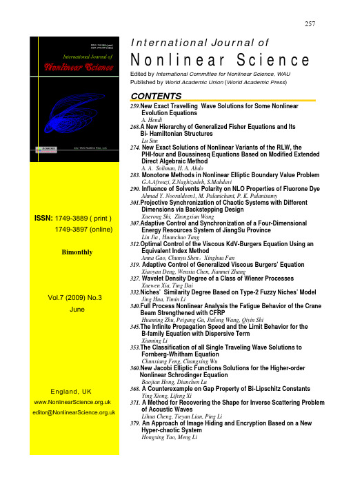
257ISSN: 1749-3889 ( print ) 1749-3897 (online)BimonthlyVol.7 (2009) No.3JuneEngland, UK ***************************.uk International Journal ofN o n l i n e a r S c i e n c e Edited by International Committee for Nonlinear Science, WAUPublished by World Academic Union (World Academic Press)CONTENTS259.New Exact Travelling Wave Solutions for Some Nonlinear Evolution EquationsA. Hendi268.A New Hierarchy of Generalized Fisher Equations and Its Bi- Hamiltonian StructuresLu Sun274.New Exact Solutions of Nonlinear Variants of the RLW, the PHI-four and Boussinesq Equations Based on Modified Extended Direct Algebraic MethodA. A. Soliman, H. A. Abdo283. Monotone Methods in Nonlinear Elliptic Boundary Value ProblemG.A.Afrouzi, Z.Naghizadeh, S.Mahdavi290. Influence of Solvents Polarity on NLO Properties of Fluorone Dye Ahmad Y. Nooraldeen1, M. Palanichant, P. K. Palanisamy301.Projective Synchronization of Chaotic Systems with Different Dimensions via Backstepping DesignXuerong Shi, Zhongxian Wang307.Adaptive Control and Synchronization of a Four-Dimensional Energy Resources System of JiangSu ProvinceLin Jia , Huanchao Tang312.Optimal Control of the Viscous KdV-Burgers Equation Using an Equivalent Index MethodAnna Gao, Chunyu Shen,Xinghua Fan319.Adaptive Control of Generalized Viscous Burgers’ Equation Xiaoyan Deng, Wenxia Chen, Jianmei Zhang327. Wavelet Density Degree of a Class of Wiener Processes Xuewen Xia, Ting Dai332.Niches’ Similarity Degree Based on Type-2 Fuzzy Niches’ Model Jing Hua, Yimin Li340.Full Process Nonlinear Analysis the Fatigue Behavior of the Crane Beam Strengthened with CFRPHuaming Zhu, Peigang Gu, Jinlong Wang, Qiyin Shi345.The Infinite Propagation Speed and the Limit Behavior for the B-family Equation with Dispersive TermXiuming Li353.The Classification of all Single Traveling Wave Solutions to Fornberg-Whitham EquationChunxiang Feng, Changxing Wu360.New Jacobi Elliptic Functions Solutions for the Higher-orderNonlinear Schrodinger EquationBaojian Hong, Dianchen Lu368.A Counterexample on Gap Property of Bi-Lipschitz Constants Ying Xiong, Lifeng Xi371.A Method for Recovering the Shape for Inverse Scattering Problem of Acoustic WavesLihua Cheng, Tieyan Lian, Ping Li379.An Approach of Image Hiding and Encryption Based on a New Hyper-chaotic SystemHongxing Yao, Meng Li258International Journal of Nonlinear Science (IJNS)BibliographicISSN: 1749-3889 (print), 1749-3897 (online), BimonthlyEdited by International Editorial Committee of Nonlinear Science, WAUPublished by World Academic Union (World Academic Press)Publisher Contact:Academic House, 113 Mill LaneWavertree Technology Park, Liverpool L13 4AH, England, UKEmail:******************.uk,*********************************URL: www. World Academic Union .comContribution enquiries and submittingThe paper(s) could be submitted to the managing editor ***************************.uk. Author also can contact our editorial offices by mail or email at addresses below directly.For more detail to submit papers please visit Editorial BoardEditor in Chief: Boling Guo, Institute of Applied Physics and Computational Mathematics, Beijing, 100088, China;************.cnCo-Editor in Chief: Lixin Tian, Nonlinear Scientific Research Center, Faculty of Science, Jiangsu University, Zhenjiang, Jiangsu,212013;China;**************.cn,************.cnStanding Members of Editorial Board:Ghasem Alizahdeh Afrouzi, Department ofMathematics, Faculty of Basic Sciences, Mazandaran University,Babolsar,Iran;**************.ir Stephen Anco, Department of Mathematics, Brock University, 500 Glenridge Avenue St. Catharines, ON L2S3A1,Canada;***************Adrian Constantin ,Department of Mathematics, Lund University,22100Lund,****************.seSweden;*************************.se,Ying Fan, Department of Management Science, Institute of Policy and Management, ChineseAcademy of Sciences, Beijing 100080,China,**************.cn.Juergen Garloff, University of Applied Sciences/ HTWG Konstanz, Faculty of Computer Science, Postfach100543, D-78405 Konstanz, Germany;************************Tasawar Hayat, Department of mathematics,Quaid-I-AzamUniversity,Pakistan,*****************Y Jiang, William Lee Innovation Center, University of Manchester, Manchester, M60 1QD UK;*******************Zhujun Jing,Institute of Mathematics, Academy of Mathematics and Systems Sciences, ChineseAcademy of Science, Beijing, 100080,China;******************Yue Liu,Department of Mathematics, University of Texas, Arlington,TX76019,USA;************Zengrong Liu,Department of Mathematics, Shanghai University, Shanghai, 201800,China;******************.cnNorio Okada, Disaster Prevention Research Institute, KyotoUniversity,****************.kyoto-u.ac.jp Jacques Peyriere,Université Paris-Sud, Mathématique, bˆa t. 42591405 ORSAY Cedex , France;************************,****************************.frWeiyi Su, Department of Mathematics, NanjingUniversity, Nanjing,Jiangsu, 210093,China;*************.cnKonstantina Trivisa ,Department of Mathematics, University of Maryland College Park,MD20472-4015,USA;****************.eduYaguang Wang,Department of Mathematics, Shanghai Jiao Tong University, Shanghai, 200240,China;***************.cnAbdul-Majid Wazwaz, 3700 W. 103rd Street Department of Mathematics and Computer Science, Saint Xavier University, Chicago, IL 60655 ,USA;**************Yiming Wei, Institute of Policy and management, Chinese Academy of Science, Beijing, 100080,China;*****************Zhiying Wen,Department of Mathematics, Tsinghua University, Beijing, 100084, China;*******************Zhenyuan Xu, Faculty of Science, Southern Yangtze University, Wuxi , Jiangsu 214063 ,China;*********************Huicheng Yi n, Department of Mathematics, Nanjing University, Nanjing, Jiangsu, 210093, China;****************.cnPingwen Zhang, School of Mathematic Sciences, Peking University, Beijing, 100871, China;**************.cnSecretary: Xuedi Wang, Xinghua FanEditorial office:Academic House, 113 Mill Lane Wavertree Technology Park Liverpool L13 4AH, England, UK Email:***************************.uk **************************.uk ************.cn。
微积分介值定理的英文
微积分介值定理的英文The Intermediate Value Theorem in CalculusCalculus, a branch of mathematics that has revolutionized the way we understand the world around us, is a vast and intricate subject that encompasses numerous theorems and principles. One such fundamental theorem is the Intermediate Value Theorem, which plays a crucial role in understanding the behavior of continuous functions.The Intermediate Value Theorem, also known as the Bolzano Theorem, states that if a continuous function takes on two different values, then it must also take on all values in between those two values. In other words, if a function is continuous on a closed interval and takes on two different values at the endpoints of that interval, then it must also take on every value in between those two endpoint values.To understand this theorem more clearly, let's consider a simple example. Imagine a function f(x) that represents the height of a mountain as a function of the distance x from the base. If the function f(x) is continuous and the mountain has a peak, then theIntermediate Value Theorem tells us that the function must take on every height value between the base and the peak.Mathematically, the Intermediate Value Theorem can be stated as follows: Let f(x) be a continuous function on a closed interval [a, b]. If f(a) and f(b) have opposite signs, then there exists a point c in the interval (a, b) such that f(c) = 0.The proof of the Intermediate Value Theorem is based on the properties of continuous functions and the completeness of the real number system. The key idea is that if a function changes sign on a closed interval, then it must pass through the value zero somewhere in that interval.One important application of the Intermediate Value Theorem is in the context of finding roots of equations. If a continuous function f(x) changes sign on a closed interval [a, b], then the Intermediate Value Theorem guarantees that there is at least one root (a value of x where f(x) = 0) within that interval. This is a powerful tool in numerical analysis and the study of nonlinear equations.Another application of the Intermediate Value Theorem is in the study of optimization problems. When maximizing or minimizing a continuous function on a closed interval, the Intermediate Value Theorem can be used to establish the existence of a maximum orminimum value within that interval.The Intermediate Value Theorem is also closely related to the concept of connectedness in topology. If a function is continuous on a closed interval, then the image of that interval under the function is a connected set. This means that the function "connects" the values at the endpoints of the interval, without any "gaps" in between.In addition to its theoretical importance, the Intermediate Value Theorem has practical applications in various fields, such as economics, biology, and physics. For example, in economics, the theorem can be used to show the existence of equilibrium prices in a market, where supply and demand curves intersect.In conclusion, the Intermediate Value Theorem is a fundamental result in calculus that has far-reaching implications in both theory and practice. Its ability to guarantee the existence of values between two extremes has made it an indispensable tool in the study of continuous functions and the analysis of complex systems. Understanding and applying this theorem is a crucial step in mastering the powerful concepts of calculus.。
newton迭代法11-12

若f(a)f(x0)<0 成立,则根必在区间(a, x0)内,取a1=a,b1= x0;否则 必在区间(x0,b)内,取a1= x0,b1=b,
这样,得到新区间(a1,b1),其长度为[a,b]的一半,如此继续下去,进 行k次等分后,得到一组不断缩小的区间,[a,b],[a1,b1],......[ak,bk].
( x*)
2!
( x x*) 2
( p1) ( x*)
( p 1)!
( x x*)p1
( p ) ( x*)
p!
( x x*)p
如果( x*) ( x*) ( p1) ( x*) 0
而 ( p ) ( x*) 0
解三:迭代格式 xk+1=(xk3-5)/2 令x0=2.5,得迭代序列: x1=5.3125, x2=72.46643066, X3=190272.0118, x4=3.444250536 1016, x5=2.042933398 1046, 计算x6时溢出
同样的方程不同的迭代格式有不同的结果 迭代函数的构造有关
L Lk xk x * xk xk 1 x1 x0 1 L 1 L
xk x * x * xk 1 xk xk 1 g'( ) xk x * xk xk+1
因此: 1 xk x * xk xk+1 1 L
证毕.
定理1指出,
例1 用简单迭代法求区间(2,3)内方程x3-2x-5=0的根 lim x 解一 将方程两边同加2x+5,再开三次方,得式同解方程 x= 3 2 x 5 作迭代格式 xk+1= 3 2 xk 5 , k=0,1,
SAT考试备考数学题目19. nonlinear equation graphs

17. An exponential function is graphed in the xy-plane below. Which of the following equations could represent the graph?
A. f(x) =5(x−2)2+3 B. f(x) =5(x+2)2+3 C. f(x) =−5(x−2)2+3 D. f(x) =−5(x+2)2+3
Correct Answer: D Difficult Level: 3
20. Which of the following shows the graph of the equation y=2(x+1)2−5?
Correct Answer: C Difficult Level: 2
12.
The functions f(x)=√ 3 −4 and g(x)= √ above. What is the value of b?
3+b are graphed in the xy-plane
Correct Answer: 5 13.
8.
The system of equations represented by the graph above is: y=−(x+3)2+5 y=x+6
If (−5,b) is a solution to the system, then what is the value of b?
Correct Answer: 1 Difficult Level: 2 9. The functions y=3(x+2)2−4 and y=−3(x+2)2−4 are graphed in the xy-plane. Which of the following must be true of the graphs of the vertexes and axes of symmetry of the two functions? Please choose from one of the following options. A. The functions will have different vertexes. B. The functions will have different axes of symmetry. C. The function y=3(x+2)2−4 will have a minimum value, and the function y=−3(x+2)2−4 will have a maximum value. D. The function y=3(x+2)2−4 will have a maximum value, and the graph of y=3(x+2)2-4 will have a minimum value.
nonlinear systems
CPx
= UCP, CPt = VCP,
(2.1b)
where the Jost function cP and U and Vare complex matrix functions of the field q, its derivatives, independent variables x and t, and the spectral parameter A. The integrability of (2.1a), which is equivalent to the flatness condition, requires that the following two-form e should vanish: (2.2a) where A denotes exterior product. In component form the compatibility condition CPxt = CPtx' which is equivalent to (2.2a), is given by
II. GAUGE EQUIVALENCE OF NONLINEAR EVOLUTIONARY SYSTEMS
where d denotes exterior differentiation, fl is a I-form matrix valued on the Lie algebra of some matrix group G, and u is the matrix O-form. In (1 + 1) space-time, Eq. (2.1a) in the component form looks as
e=
dfl - fl A fl = 0 ,
- 1、下载文档前请自行甄别文档内容的完整性,平台不提供额外的编辑、内容补充、找答案等附加服务。
- 2、"仅部分预览"的文档,不可在线预览部分如存在完整性等问题,可反馈申请退款(可完整预览的文档不适用该条件!)。
- 3、如文档侵犯您的权益,请联系客服反馈,我们会尽快为您处理(人工客服工作时间:9:00-18:30)。
C H A P T E R11 Nonlinear EquationsIn many applications we do not need to optimize an objective function explicitly,but rather tofind values of the variables in a model that satisfy a number of given relationships.When these relationships take the form of n equalities—the same number of equality conditions as variables in the model—the problem is one of solving a system of nonlinear equations. We write this problem mathematically asr(x) 0,(11.1)C H A P T E R11.N O N L I N E A R E Q U A T I O N S271 where r:I R n→I R n is a vector function,that is,r(x) ⎡⎢⎢⎢⎢⎢⎣r1(x)r2(x)...r n(x)⎤⎥⎥⎥⎥⎥⎦.In this chapter,we assume that each function r i:I R n→I R,i 1,2,...,n,is smooth.A vector x∗for which(11.1)is satisfied is called a solution or root of the nonlinear equations.A simple example is the systemr(x)x22−1sin x1−x20,which is a system of n 2equations with infinitely many solutions,two of which are x∗ (3π/2,−1)T and x∗ (π/2,1)T.In general,the system(11.1)may have no solutions, a unique solution,or many solutions.The techniques for solving nonlinear equations overlap in their motivation,analysis, and implementation with optimization techniques discussed in earlier chapters.In both optimization and nonlinear equations,Newton’s method lies at the heart of many important algorithms.Features such as line searches,trust regions,and inexact solution of the linear algebra subproblems at each iteration are important in both areas,as are other issues such as derivative evaluation and global convergence.Because some important algorithms for nonlinear equations proceed by minimizing a sum of squares of the equations,that is,min xni 1r2i(x),there are particularly close connections with the nonlinear least-squares problem discussed in Chapter10.The differences are that in nonlinear equations,the number of equations equals the number of variables(instead of exceeding the number of variables,as is typically the case in Chapter10),and that we expect all equations to be satisfied at the solution,rather than just minimizing the sum of squares.This point is important because the nonlinear equations may represent physical or economic constraints such as conservation laws or consistency principles,which must hold exactly in order for the solution to be meaningful.Many applications require us to solve a sequence of closely related nonlinear systems, as in the following example.272C H A P T E R11.N O N L I N E A R E Q U A T I O N S❏E XAMPLE11.1(R HEINBOLDT;SEE[212])An interesting problem in control is to analyze the stability of an aircraft in response to the commands of the pilot.The following is a simplified model based on force-balance equations,in which gravity terms have been neglected.The equilibrium equations for a particular aircraft are given by a system of5equations in8unknowns of the formF(x)≡Ax+φ(x) 0,(11.2) where F:I R8→I R5,the matrix A is given byA ⎡⎢⎢⎢⎢⎢⎢⎣−3.9330.1070.1260−9.990−45.83−7.64 0−0.9870−22.950−28.37000.0020−0.23505.670−0.921−6.5101.00−1.00−0.1680000−1.00−0.1960−0.00710⎤⎥⎥⎥⎥⎥⎥⎦,and the nonlinear part is defined byφ(x) ⎡⎢⎢⎢⎢⎢⎢⎢⎣−0.727x2x3+8.39x3x4−684.4x4x5+63.5x4x20.949x1x3+0.173x1x5−0.716x1x2−1.578x1x4+1.132x4x2−x1x5x1x4⎤⎥⎥⎥⎥⎥⎥⎥⎦.Thefirst three variables x1,x2,x3,represent the rates of roll,pitch,and yaw,respec-tively,while x4is the incremental angle of attack and x5the sideslip angle.The last three variables x6,x7,x8are the controls;they represent the deflections of the elevator,aileron, and rudder,respectively.For a given choice of the control variables x6,x7,x8we obtain a system of5equations and5unknowns.If we wish to study the behavior of the aircraft as the controls are changed, we need to solve a system of nonlinear equations with unknowns x1,x2,...,x5for each setting of the controls.❐Despite the many similarities between nonlinear equations and unconstrained and least-squares optimization algorithms,there are also some important differences.To ob-tain quadratic convergence in optimization we require second derivatives of the objective function,whereas knowledge of thefirst derivatives is sufficient in nonlinear equations.C H A P T E R11.N O N L I N E A R E Q U A T I O N S273Figure11.1The function r(x) sin(5x)−x has three roots.Quasi-Newton methods are perhaps less useful in nonlinear equations than in optimiza-tion.In unconstrained optimization,the objective function is the natural choice of merit function that gauges progress towards the solution,but in nonlinear equations various merit functions can be used,all of which have some drawbacks.Line search and trust-region tech-niques play an equally important role in optimization,but one can argue that trust-region algorithms have certain theoretical advantages in solving nonlinear equations.Some of the difficulties that arise in trying to solve nonlinear equations can be illustrated by a simple scalar example(n 1).Suppose we haver(x) sin(5x)−x,(11.3)as plotted in Figure11.1.From thisfigure we see that there are three solutions of the problem r(x) 0,also known as roots of r,located at zero and approximately±0.519148.This situation of multiple solutions is similar to optimization problems where,for example,a function may have more than one local minimum.It is not quite the same,however:Inthe case of optimization,one of the local minima may have a lower function value thanthe others(making it a“better”solution),while in nonlinear equations all solutions are equally good from a mathematical viewpoint.(If the modeler decides that the solution274C H A P T E R11.N O N L I N E A R E Q U A T I O N Sfound by the algorithm makes no sense on physical grounds,their model may need to be reformulated.)In this chapter we start by outlining algorithms related to Newton’s method and examining their local convergence properties.Besides Newton’s method itself,these in-clude Broyden’s quasi-Newton method,inexact Newton methods,and tensor methods.We then address global convergence,which is the issue of trying to force convergence toa solution from a remote starting point.Finally,we discuss a class of methods in whichan“easy”problem—one to which the solution is well known—is gradually transformed into the problem F(x) 0.In these so-called continuation(or homotopy)methods,we track the solution as the problem changes,with the aim offinishing up at a solution of F(x) 0.Throughout this chapter we make the assumption that the vector function r is con-tinuously differentiable in the region D containing the values of x we are interested in.In other words,the Jacobian J(x)(the matrix offirst partial derivatives of r(x)defined in the Appendix and in(10.3))exists and is continuous.We say that x∗satisfying r(x∗) 0is a degenerate solution if J(x∗)is singular,and a nondegenerate solution otherwise.11.1LOCAL ALGORITHMSNEWTON’S METHOD FOR NONLINEAR EQUATIONSRecall from Theorem2.1that Newton’s method for minimizing f:I R n→I R forms a quadratic model function by taking thefirst three terms of the Taylor series approximation of f around the current iterate x k.The Newton step is the vector that minimizes this model.In the case of nonlinear equations,Newton’s method is derived in a similar way,but with a linear model,one that involves function values andfirst derivatives of the functions r i(x),i 1,2,...,m at the current iterate x k.We justify this strategy by referring to the followingmultidimensional variant of Taylor’s theorem.Theorem11.1.Suppose that r:I R n→I R n is continuously differentiable in some convex open set D and that x and x+p are vectors in D.We then have that1r(x+p) r(x)+J(x+tp)p dt.(11.4)We can define a linear model M k(p)of r(x k+p)by approximating the second term on the right-hand-side of(11.4)by J(x)p,and writingM k(p)def r(x k)+J(x k)p.(11.5)11.1.L O C A L A L G O R I T H M S275 Newton’s method,in its pure form,chooses the step p k to be the vector for which M k(p k)0,that is,p k −J(x k)−1r(x k).We define it formally as follows.Algorithm11.1(Newton’s Method for Nonlinear Equations).Choose x0;for k 0,1,2,...Calculate a solution p k to the Newton equationsJ(x k)p k −r(x k);(11.6) x k+1←x k+p k;end(for)We use a linear model to derive the Newton step,rather than a quadratic model as in unconstrained optimization,because the linear model normally has a solution and yields an algorithm with rapid convergence properties.In fact,Newton’s method for unconstrained optimization(see(2.15))can be derived by applying Algorithm11.1to the nonlinear equations∇f(x) 0.We see also in Chapter18that sequential quadratic programmingfor equality-constrained optimization can be derived by applying Algorithm11.1to the nonlinear equations formed by thefirst-order optimality conditions(18.3)for this problem. Another connection is with the Gauss–Newton method for nonlinear least squares;the formula(11.6)is equivalent to(10.23)in the usual case in which J(x k)is nonsingular.When the iterate x k is close to a nondegenerate root x∗,Newton’s method converges superlinearly,as we show in Theorem11.2below.Potential shortcomings of the method include the following.•When the starting point is remote from a solution,Algorithm11.1can behaveerratically.When J(x k)is singular,the Newton step may not even be defined.•First-derivative information(the Jacobian matrix J)may be difficult to obtain.•It may be too expensive tofind and calculate the Newton step p k exactly when n islarge.•The root x∗in question may be degenerate,that is,J(x∗)may be singular.An example of a degenerate problem is the scalar function r(x) x2,which has a single degenerate root at x∗ 0.Algorithm11.1,when started from any nonzero x0,generates the sequence of iteratesx k 12x0,which converges to the solution0,but only at a linear rate.As we show later in this chapter,Newton’s method can be modified and enhanced in various ways to get around most of these problems.The variants we describe form the basis of much of the available software for solving nonlinear equations.276C H A P T E R11.N O N L I N E A R E Q U A T I O N SWe summarize the local convergence properties of Algorithm11.1in the following theorem.For part of this result,we make use of a Lipschitz continuity assumption on the Jacobian,by which we mean that there is a constantβL such thatJ(x0)−J(x1) ≤βL x0−x1 ,(11.7) for all x0and x1in the domain in question.Theorem11.2.Suppose that r is continuously differentiable in a convex open set D⊂I R n.Let x∗∈D be a nondegenerate solution of r(x) 0,and let{x k}be the sequence of iterates generated by Algorithm11.1.Then when x k∈D is sufficiently close to x∗,we havex k+1−x∗ o( x k−x∗ ),(11.8) indicating local Q-superlinear convergence.When r is Lipschitz continuously differentiable near x∗,we have for all x k sufficiently close to x∗thatx k+1−x∗ O( x k−x∗ 2),(11.9) indicating local Q-quadratic convergence.P ROOF.Since r(x∗) 0,we have from Theorem11.1thatr(x k) r(x k)−r(x∗) J(x k)(x k−x∗)+w(x k,x∗),(11.10) wherew(x k,x∗) 1J(x k+t(x∗−x k))−J(x k)(x k−x∗).(11.11)From(A.12)and continuity of J,we havew(x k,x∗)1[J(x∗+t(x∗−x k))−J(x k)](x k−x∗)dt≤ 1J(x∗+t(x∗−x k))−J(x k) x k−x∗ dt(11.12)o( x k−x∗ ).Since J(x∗)is nonsingular,there is a radiusδ>0and a positive constantβ∗such that for all x in the ball B(x∗,δ)defined byB(x∗,δ) {x| x−x∗ ≤δ},(11.13)11.1.L O C A L A L G O R I T H M S277we have thatJ(x)−1 ≤β∗and x∈D.(11.14) Assuming that x k∈B(x∗,δ),and recalling the definition(11.6),we multiply both sides of (11.10)by J(x k)−1to obtain−p k (x k−x∗)+ J(x k)−1 o( x k−x∗ ),⇒x k+p k−x∗ o( x k−x∗ ),⇒x k+1−x∗ o( x k−x∗ ),(11.15) which yields(11.8).When the Lipschitz continuity assumption(11.7)is satisfied,we can obtain a sharper estimate for the remainder term w(x k,x∗)defined in(11.11).By using(11.7)in(11.12),we obtainw(x k,x∗) O( x k−x∗ 2).(11.16)By multiplying(11.10)by J(x k)−1as above,we obtain−p k−(x k−x∗) J(x k)−1w(x k,x∗),so the estimate(11.9)follows as in(11.15).INEXACT NEWTON METHODSInstead of solving(11.6)exactly,inexact Newton methods use search directions p kthat satisfy the conditionr k+J k p k ≤ηk r k ,for someηk∈[0,η],(11.17) whereη∈[0,1)is a constant.As in Chapter7,we refer to{ηk}as the forcing sequence. Different methods make different choices of the forcing sequence,and they use different algorithms forfinding the approximate solutions p k.The general framework for this classof methods can be stated as follows.Framework11.2(Inexact Newton for Nonlinear Equations).Givenη∈[0,1);Choose x0;for k 0,1,2,...Choose forcing parameterηk∈[0,η];Find a vector p k that satisfies(11.17);x k+1←x k+p k;end(for)278C H A P T E R11.N O N L I N E A R E Q U A T I O N SThe convergence theory for these methods depends only on the condition(11.17) and not on the particular technique used to calculate p k.The most important methods in this class,however,make use of iterative techniques for solving linear systems of the form J p −r,such as GMRES(Saad and Schultz[273],Walker[302])or other Krylov-space methods.Like the conjugate-gradient algorithm of Chapter5(which is not directly applicable here,since the coefficient matrix J is not symmetric positive definite),these methods typically require us to perform a matrix–vector multiplication of the form Jd for some d at each iteration,and to store a number of work vectors of length n.GMRES requires an additional vector to be stored at each iteration,so must be restarted periodically(often every10or20iterations)to keep memory requirements at a reasonable level.The matrix–vector products Jd can be computed without explicit knowledge of the Jacobian J.Afinite-difference approximation to Jd that requires one evaluation of r(·) is given by the formula(8.11).Calculation of Jd exactly(at least,to within the limits of finite-precision arithmetic)can be performed by using the forward mode of automatic differentiation,at a cost of at most a small multiple of an evaluation of r(·).Details of this procedure are given in Section8.2.We do not discuss the iterative methods for sparse linear systems here,but refer the interested reader to Kelley[177]and Saad[272]for comprehensive descriptions and implementations of the most interesting techniques.We prove a local convergence theorem for the method,similar to Theorem11.2.Theorem11.3.Suppose that r is continuously differentiable in a convex open set D⊂I R n.Let x∗∈D be a nondegenerate solution of r(x) 0,and let{x k}be the sequence of iterates generated by the Framework11.2.Then when x k∈D is sufficiently close to x∗,the following are true:(i)Ifηin(11.17)is sufficiently small,the convergence of{x k}to x∗is Q-linear.(ii)Ifηk→0,the convergence is Q-superlinear.(iii)If,in addition,J(·)is Lipschitz continuous in a neighborhood of x∗andηk O( r k ), the convergence is Q-quadratic.P ROOF.Wefirst rewrite(11.17)asJ(x k)p k+r(x k) v k,where v k ≤ηk r(x k) .(11.18) Since x∗is a nondegenerate root,we have as in(11.14)that there is a radiusδ>0such that J(x)−1 ≤β∗for some constantβ∗and all x∈B(x∗,δ).By multiplying both sides of(11.18)by J(x k)−1and rearranging,wefind thatp k+J(x k)−1r(x k)J(x k)−1v k≤β∗ηk r(x k) .(11.19)11.1.L O C A L A L G O R I T H M S 279As in (11.10),we have thatr (x ) J (x )(x −x ∗)+w (x ,x ∗),(11.20)where ρ(x )def w (x ,x ∗) / x −x ∗ →0as x →x ∗.By reducing δif necessary,we have from this expression that the following bound holds for all x ∈B (x ∗,δ):r (x ) ≤2 J (x ∗) x −x ∗ +o ( x −x ∗ )≤4 J (x ∗) x −x ∗ .(11.21)We now set x x k in (11.20),and use (11.19)and (11.21)to obtainx k +p k −x ∗ p k +J (x k )−1(r (x k )−w (x k ,x ∗))≤β∗ηk r (x k ) + J (x k )−1 w (x k ,x ∗) ≤ 4 J (x ∗) β∗ηk +β∗ρ(x k ) x k −x ∗ .(11.22)By choosing x k close enough to x ∗that ρ(x k )≤1/(4β∗),and choosing η 1/(8 J (x ∗) β∗),we have that the term in square brackets in (11.22)is at most 1/2.Hence,since x k +1 x k +p k ,this formula indicates Q-linear convergence of {x k }to x ∗,proving part (i).Part (ii)follows immediately from the fact that the term in brackets in (11.22)goes to zero as x k →x ∗and ηk →0.For part (iii),we combine the techniques above with the logic of the second part of the proof of Theorem 11.2.Details are left as an exercise.BROYDEN’S METHODSecant methods,also known as quasi-Newton methods,do not require calculation of the Jacobian J (x ).Instead,they construct their own approximation to this matrix,updating it at each iteration so that it mimics the behavior of the true Jacobian J over the step just taken.The approximate Jacobian,which we denote at iteration k by B k ,is then used to construct a linear model analogous to (11.5),namelyM k (p ) r (x k )+B k p .(11.23)We obtain the step by setting this model to zero.When B k is nonsingular,we have the following explicit formula (cf.(11.6)):p k −B −1k r (x k ).(11.24)The requirement that the approximate Jacobian should mimic the behavior of the true Jacobian can be specified as follows.Let s k denote the step from x k to x k +1,and let y k280C H A P T E R11.N O N L I N E A R E Q U A T I O N Sbe the corresponding change in r,that is,s k x k+1−x k,y k r(x k+1)−r(x k).(11.25) From Theorem11.1,we have that s k and y k are related by the expressiony k 1J(x k+ts k)s k dt≈J(x k+1)s k+o( s k ).(11.26)We require the updated Jacobian approximation B k+1to satisfy the following equation, which is known as the secant equation,y k B k+1s k,(11.27) which ensures that B k+1and J(x k+1)have similar behavior along the direction s k.(Note the similarity with the secant equation(6.6)in quasi-Newton methods for unconstrained optimization;the motivation is the same in both cases.)The secant equation does not say anything about how B k+1should behave along directions orthogonal to s k.In fact,we can view(11.27)as a system of n linear equations in n2unknowns,where the unknowns are the components of B k+1,so for n>1the equation(11.27)does not determine all the components of B k+1uniquely.(The scalar case of n 1gives rise to the scalar secant method;see(A.60).)The most successful practical algorithm is Broyden’s method,for which the update formula isB k+1 B k+(y k−B k s k)s T ks Tks k.(11.28)The Broyden update makes the smallest possible change to the Jacobian(as measured by the Euclidean norm B k−B k+1 2)that is consistent with(11.27),as we show in the following Lemma.Lemma11.4(Dennis and Schnabel[92,Lemma8.1.1]).Among all matrices B satisfying Bs k y k,the matrix B k+1defined by(11.28)minimizes the difference B−B k .P ROOF.Let B be any matrix that satisfies Bs k y k.By the properties of the Euclidean norm(see(A.10))and the fact that ss T/s T s 1for any vector s(see Exercise11.1),we haveB k+1−B k(y k−B k s k)s T ks Tks k(B−B k)s k s T ks Tks k≤ B−Bks k s T ks Tks kB−Bk .11.1.L O C A L A L G O R I T H M S281 Hence,we have thatB k+1∈arg minB:y k Bs kB−B k ,and the result is proved.In the specification of the algorithm below,we allow a line search to be performed along the search direction p k,so that s k αp k for someα>0in the formula(11.25).(See below for details about line-search methods.)Algorithm11.3(Broyden).Choose x0and a nonsingular initial Jacobian approximation B0;for k 0,1,2,...Calculate a solution p k to the linear equationsB k p k −r(x k);(11.29)Chooseαk by performing a line search along p k;x k+1←x k+αk p k;s k←x k+1−x k;y k←r(x k+1)−r(x k);Obtain B k+1from the formula(11.28);end(for)Under certain assumptions,Broyden’s method converges superlinearly,that is,x k+1−x∗ o( x k−x∗ ).(11.30)This local convergence rate is fast enough for most practical purposes,though not as fast asthe Q-quadratic convergence of Newton’s method.We illustrate the difference between the convergence rates of Newton’s and Broyden’s method with a small example.The function r:I R2→I R2defined byr(x)(x1+3)(x32−7)+18sin(x2e x1−1)(11.31)has a nondegenerate root at x∗ (0,1)T.We start both methods from the point x0 (−0.5,1.4)T,and use the exact Jacobian J(x0)at this point as the initial Jacobian approximation B0.Results are shown in Table11.1.Newton’s method clearly exhibits Q-quadratic convergence,which is characterized by doubling of the exponent of the error at each iteration.Broyden’s method takes twice as282C H A P T E R11.N O N L I N E A R E Q U A T I O N STable11.1Convergence of Iterates in Broydenand Newton Methodsx k−x∗ 2Iteration k Broyden Newton00.64×1000.64×10010.62×10−10.62×10−120.52×10−30.21×10−330.25×10−30.18×10−740.43×10−40.12×10−1550.14×10−660.57×10−970.18×10−1180.87×10−15Table11.2Convergence of Function Norms inBroyden and Newton Methodsr(x k) 2Iteration k Broyden Newton00.74×1010.74×10110.59×1000.59×10020.20×10−20.23×10−230.21×10−20.16×10−640.37×10−30.22×10−1550.12×10−560.49×10−870.15×10−1080.11×10−18many iterations as Newton’s,and reduces the error at a rate that accelerates slightly towards the end.The function norms r(x k) approach zero at a similar rate to the iteration errors x k−x∗ .As in(11.10),we have thatr(x k) r(x k)−r(x∗)≈J(x∗)(x k−x∗),so by nonsingularity of J(x∗),the norms of r(x k)and(x k−x∗)are bounded above and below by multiples of each other.For our example problem(11.31),convergence of the sequence of function norms in the two methods is shown in Table11.2.The convergence analysis of Broyden’s method is more complicated than that of Newton’s method.We state the following result without proof.Theorem11.5.Suppose the assumptions of Theorem11.2hold.Then there are positive constants and δsuch that if the starting point x0and the starting approximate Jacobian B0satisfyx0−x∗ ≤δ, B0−J(x∗) ≤ ,(11.32)11.1.L O C A L A L G O R I T H M S283 the sequence{x k}generated by Broyden’s method(11.24),(11.28)is well-defined and convergesQ-superlinearly to x∗.The second condition in(11.32)—that the initial Jacobian approximation B0mustbe close to the true Jacobian at the solution J(x∗)—is difficult to guarantee in practice.In contrast to the case of unconstrained minimization,a good choice of B0can be crit-ical to the performance of the algorithm.Some implementations of Broyden’s method recommend choosing B0to be J(x0),or somefinite-difference approximation to this matrix.The Broyden matrix B k will be dense in general,even if the true Jacobian J is sparse. Therefore,when n is large,an implementation of Broyden’s method that stores B k as a fulln×n matrix may be inefficient.Instead,we can use limited-memory methods in whichB k is stored implicitly in the form of a number of vectors of length n,while the system(11.29)is solved by a technique based on application of the Sherman–Morrison–Woodbury formula(A.28).These methods are similar to the ones described in Chapter7for large-scale unconstrained optimization.TENSOR METHODSIn tensor methods,the linear model M k(p)used by Newton’s method(11.5)is aug-mented with an extra term that aims to capture some of the nonlinear,higher-order, behavior of r.By doing so,it achieves more rapid and reliable convergence to degenerate roots,in particular,to roots x∗for which the Jacobian J(x∗)has rank n−1or n−2.We give a broad outline of the method here,and refer to Schnabel and Frank[277]for details.We useˆM k(p)to denote the model function on which tensor methods are based;this function has the formˆM k (p) r(x k)+J(x k)p+12T k pp,(11.33)where T k is a tensor defined by n3elements(T k)i jl whose action on a pair of arbitrary vectors u and v in I R n is defined by(T k u v)inj 1nl 1(T k)i jl u j v l.If we followed the reasoning behind Newton’s method,we could consider building T k from the second derivatives of r at the point x k,that is,(T k)i jl [∇2r i(x k)]jl.284C H A P T E R 11.N O N L I N E A R E Q U A T I O N SFor instance,in the example (11.31),we have that(T (x )u v )1 u T ∇2r 1(x )v u T3x 223x 226x 2(x 1+3)v 3x 22(u 1v 2+u 2v 1)+6x 2(x 1+3)u 2v 2.However,use of the exact second derivatives is not practical in most instances.If we were to store this information explicitly,about n 3/2memory locations would be needed,about n times the requirements of Newton’s method.Moreover,there may be no vector p for which ˆMk (p ) 0,so the step may not even be defined.Instead,the approach described in [277]defines T k in a way that requires little additional storage,but which gives ˆM k some potentially appealing properties.Specifically,T k is chosen so that ˆMk (p )interpolates the function r (x k +p )at some previous iterates visited by the algorithm.That is,we require thatˆM k (x k −j −x k ) r (x k −j ),for j 1,2,...,q ,(11.34)for some integer q >0.By substituting from (11.33),we see that T k must satisfy the condition 1T k s jk s jk r (x k −j )−r (x k )−J (x k )s jk ,wheres jk defx k −j −x k ,j 1,2,...,q .In [277]it is shown that this condition can be ensured by choosing T k so that its action on arbitrary vectors u and v isT k u v qj 1a j (s T jk u )(s T jk v ),where a j ,j 1,2,...,q ,are vectors of length n .The number of interpolating points q is typically chosen to be quite modest,usually less than √n .This T k can be stored in 2nq locations,which contain the vectors a j and s jk for j 1,2,...,q .Note the connection between this idea and Broyden’s method,which also chooses information in the model (albeit in the first-order part of the model)to interpolate the function value at the previous iterate.This technique can be refined in various ways.The points of interpolation can be chosen to make the collection of directions s jk more linearly independent.There may still not be a vector p for which ˆMk (p ) 0,but we can instead take the step to be the vector that11.2.P R A C T I C A L M E T H O D S285 minimizes ˆM k(p) 22,which can be found by using a specialized least-squares technique. There is no assurance that the step obtained in this way is a descent direction for the meritfunction12 r(x) 2(which is discussed in the next section),and in this case it can be replacedby the standard Newton direction−J−1k r k.11.2PRACTICAL METHODSWe now consider practical variants of the Newton-like methods discussed above,in which line-search and trust-region modifications to the steps are made in order to ensure better global convergence behavior.MERIT FUNCTIONSAs mentioned above,neither Newton’s method(11.6)nor Broyden’s method(11.24), (11.28)with unit step lengths can be guaranteed to converge to a solution of r(x) 0unless they are started close to that solution.Sometimes,components of the unknown or function vector or the Jacobian will blow up.Another,more exotic,kind of behavior is cycling,where the iterates move between distinct regions of the parameter space without approaching a root.An example is the scalar functionr(x) −x5+x3+4x,which hasfive nondegenerate roots.When started from the point x0 1,Newton’s method produces a sequence of iterates that oscillates between1and−1(see Exercise11.3)without converging to any of the roots.The Newton and Broyden methods can be made more robust by using line-search and trust-region techniques similar to those described in Chapters3and4.Before describing these techniques,we need to define a merit function,which is a scalar-valued function of x that indicates whether a new iterate is better or worse than the current iterate,in the sense of making progress toward a root of r.In unconstrained optimization,the objective function f is itself a natural merit function;most algorithms for minimizing f require a decrease in f at each iteration.In nonlinear equations,the merit function is obtained by combining the n components of the vector r in some way.The most widely used merit function is the sum of squares,defined byf(x) 12 r(x) 2 12ni 1r2i(x).(11.35)(The factor1/2is introduced for convenience.)Any root x∗of r obviously has f(x∗) 0, and since f(x)≥0for all x,each root is a minimizer of f.However,local minimizers of f are not roots of r if f is strictly positive at the point in question.Still,the merit function。