CS Project Report
cs模式报表使用简介
cs模式报表使用简介java应用有不少是C/S模式,在C/S模式下,同样可以调用报表的API接口运算、展现、导出、打印报表。
报表的计算、导出和在B/S模式下方法相同。
展现和打印用到了CSReport类。
CSReport是C/S模式下的报表控件类,在这个类中可以获得报表的显示面板、获得报表的打印面板、显示报表打印窗口、直接打印报表等等。
下面分别介绍这几步的实现方法运算报表private IReport CalcReport(String reportFile, String license) {ExtCellSet.setLicenseFileName(license);//设置授权ReportDefine rd = null;try {rd = (ReportDefine) ReportUtils.read(reportFile);//读取报表 } catch (Exception e) {e.printStackTrace();}Context cxt = new Context();Engine engine = new Engine(rd, cxt);IReport iReport = engine.calc();return iReport;}以上代码的功能是运算报表,和在B/S模式下运算报表差不多。
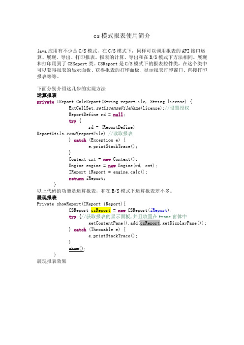
展现报表Private showReport(IReport iReport){CSReport csReport = new CSReport(iReport);try {//获取报表的显示面板,并且放置在frame窗体中getContentPane().add(csReport.getDisplayPane());} catch (Throwable e) {e.printStackTrace();}show();}展现报表效果导出报表(导出excel方法)private void SaveAsExcel() {String fileName = "";// 定义导出文件的格式FileNameExtensionFilter filter = newFileNameExtensionFilter("excel","xls");JFileChooser jFileChooser = new JFileChooser();jFileChooser.setFileSelectionMode(JFileChooser.DIRECTORIES_ONL Y);jFileChooser.setFileFilter(filter); // 调用定义好的文件类型jFileChooser.setDialogTitle("选择保存路径");int result = jFileChooser.showSaveDialog(csReport.this);if (result == JFileChooser.APPROVE_OPTION) {//判断是否选择保存按钮fileName = jFileChooser.getSelectedFile().getAbsolutePath() + ".xls";System.out.println(fileName);try {ReportUtils.exportToExcel(fileName, iReport, true);} catch (Throwable e) {e.printStackTrace();}}}其他格式文件的导出方法和这个类似,这里就不介绍了。
CS和CS与PRR

PRR:Problem Report and ResolutionPCR:Problem Communication and Report对于PRR,供方应该在24小时内给出初步答复,CKD可以在48小时内给出答复;采取的措施包括:派人到客户现场返工或者分拣;在供应商处立即采取措施以防止更多的不合格品的发运、包括收集暑假和分析;供应商必须分析整个物料链来识别和处理在客户处和正在路上的所有可疑产品;下次合格品的发运,保证客户收到合格的产品;提供供应商代表的联系信息。
在收到PRR的15天内必须给出最终答复,其中包括:已采取的遏制措施评估遏制措施有效的方法问题的根本原因(可以通过Red-X,DOE和3×5等)纠正和预防措施,比如防错遏制措施的实施步骤措施人的联系方式评估有效性的方法对解决方案的制度化、包括对类似的过程和产品的纠正文件修改记录如果问题是二级供应商造成的,对相关情况进行记录CS:受控发运CS1:由供应商在供方处实施不合格品控制,如100%检验CS2:在CS1的基础上由第三方追加实施的不合格品遏制,费用由供应商负责,客户指定第三方,这一部分费用的主要目的是惩罚!CS1进入条件:客户发布PRR后,supplier采取短期和长期措施后仍然无法遏制问题的发生;发生了重大售后质量问题的供应商实施CS1;批量性严重质量问题或类似质量问题重复发生违反PPAP程序(如擅自更改材料、分供方、工艺和检验标准等);给客户造成重大影响或损失(停线超过10分钟、DR/DRL问题发生频次超过20次;超过50分钟GCA问题)GP-12期间,在客户处发生质量缺陷同一零件发生不同质量问题3次或以上对供方的要求:立刻针对具体的质量问题,建立与现生产、检查区域独立的遏制区域;告知其他使用相同零件的顾客,告知该不合格情况,并且根据需要采用遏制行动;跟踪不合格零件的断点;在产品或产品标签上贴上绿色圆形标贴,并在其上加印CS1字样,由主管质量的最高领导签字。
cs游戏中的英语
最近发现包括相当多的CS老手在内的很多CS玩家对部分CS对讲机内的英语通话内容理解有误,鉴于此,特撰文供大家参考。
其中有些与中文版的汉字译文是不同的。
祝大家玩得更精,更开心!调用对讲机命令:按“Z”“X”“C”会看见屏幕左下角出现三组对讲电文,分别是Z系列的【无线电命令】,X系列的【队内无线电命令】和C系列的【无线电回应/报告】。
按一下“Z”后,再按一下数字“1”,你就能发出“Cover me!【掩护我!】”的语音命令。
以此类推:Z1:掩护我。
Cover me.Z2:你做先锋。
You take the point. (先锋就是排在队伍最前面的那个人,是随时准备第一个以奉献生命的方式来向排在队伍后面的队友发出敌情警报的人。
)Z3:坚守这里。
Hold this position. (两种情况需要坚守:1. 匪们安装了C4,防止警们来给拆掉,所以要坚守C4所在地点; 2. 偷袭之敌的必经之路,或者是己方撤退的必经之地,因此需要确保这个地点是安全的。
)Z4:向我集合。
Regroup team. (队伍被打散了的时候,需要重新拧成一股绳,形成战斗力,利用集中战斗力来突破某个点。
)Z5:跟我来。
Follow me.Z6:火力支援!Taking fire, need assistance! (不同于C3,既有火力掩护其逃跑或者掩护其冲锋的含义,也有要求火力增援的含义。
)X1: 冲。
Go! Go! Go!X2:回撤!Team, fall back! (可能是因为前方有烟雾弹;可能是发现前方有狙击手;可能是前方有重兵埋伏;也可能是因为屁股被包抄了。
)X3:一起走,别散开。
Stick together, team. (好处在于:1. 可以交叉掩护,各防一个方向;2. 换弹夹的时候,有人火力掩护你;3. 火力更强,比较安全。
4. 敌人潜在的伏兵只要偷袭一次,就会暴露其位置。
不至于被同一个埋伏点的敌兵逐个逐次地偷袭掉多人。
ProjectProposals

EE368/CS232 Final Project⏹Develop, implement and test/demonstrate image processing algorithm(s) ⏹May or may not use an Android device⏹Important dates●Project proposal due: April 30, 11:59 p.m.●Project presentation: Poster session, June 2, 4-6 p.m.●Submission of written report and source code: June 6, 11:59 p.m.⏹Posters, reports & source code will be posted online⏹Project grade based on●Technical quality, significance, and originality 50%●Written report 25%●Poster/demo 25%Digital Image Processing: Bernd Girod, © 2013-2014 Stanford University -- Project Proposals 1Project proposal⏹Written project proposal in pdf format⏹Submit by email to ee368-spr1314-staff@⏹Submit early for a head start, but no later than deadline⏹Proposal must contain:●Title●Name(s) and email address(es) of the student(s)●Description of the goals of the project and the work to be carried out (200-400 words)●3+ scholarly references (web pages don‘t count)●Indication whether you will use an Android device⏹We will request a revision, if needed⏹Approved proposals will be posted onlineDigital Image Processing: Bernd Girod, © 2013-2014 Stanford University -- Project Proposals 2Project group and topic⏹Groups of 2-3 students strongly encouraged⏹Groups > 3 need special permission: provide compelling reason and work plan ⏹Use our Google Doc spreadsheet and Piazza to look for project partners –indicate general direction of interest⏹Check out past proposals and projects in Final Projects section of class website ⏹Check journals and conference proceedings for ideas, e.g.,●IEEE Transactions on Image Processing●IEEE International Conference on Image Processing (ICIP)●IEEE Conference on Computer Vision and Pattern Recognition (CVPR)⏹Do not be overly ambitious in your project goals!Digital Image Processing: Bernd Girod, © 2013-2014 Stanford University -- Project Proposals 3。
cs快捷键大全
M:选择当警察还是土匪G:把手中的武器扔掉F:开启手电筒R:上子弹E:打开开关,拆包,领人质T:喷图Y:发送文字消息(所有人可见)U:发送文字消息(自己团队可见)K:对着“麦"说话大家可以听见(自己听不见)I:地图说明Z/X/C:语音命令tab:显示战绩,ping值,和玩家ID F5:抓图,自动保存在CS文件夹(BMP格式)1:切换主枪2:切换手枪3:切换刀子4:切换手雷5:切换C4W:前进S:后退A:左平移D:右平移空格:跳跃ctrl:蹲下shift:走路(默认是跑的,跑有脚步声,走路没有)CS语音命令Radio A 普通指令Z键:(注:次键为指挥键,在比赛时非指挥员误用!!!)1。
“Coer Me” 掩护我冲锋的时候需要对友的火力掩护。
2。
“YOU Take the Point” 你占据该要点让对友占据此射击点。
3。
“Hold This Position” 占据这个位置告诉对友占领此处有利地形。
4。
"Regroup Team” 重组队伍把分散的队员重新组织起来。
5。
"Follow Me" 跟随我让对友跟你一起去某处完成任务.6。
”Taking Fire,Need Assistance" 吸引火力,需要援助。
需要冲锋的时候,请求同伴吸引对方火力。
Radio B团队指令X键1。
"Go” 走,前进。
2.“Fall Back" 后退,用来通知对友一起向后撤退.3。
”Stick Together Tam" 共同作战。
4。
“Get in Position" 让对友进入指定的位置。
5.”Storm the Front” 有最快的速度,集中最强的力量打击前线。
6。
“Report ln” 用于要求对友报告他的情况。
RadioC 回答组C键1.”Affirmatie/Roger” 收到2。
.”Enemy Spotted” 发现敌人。
自动化申请CS神校,记申请那些套路

自动化申请CS神校,记申请那些套路(世毕盟学员)自身背景交大自动化系,申请CS Master【三维】GPA: 86.5TOEFL: 105,speaking 23;GRE: 156+168+3.0;【经历】自动化实验室的大创ILSVRC 2016竞赛计算机视觉和机器学习相关的科研Intel 机器学习组实习无海外经历【成果】一篇水会二作接收一篇顶会二作在投三个发明专利申请结果AD: CMU MSBIC, Columbia MSCS, UCSD MSCS, WUSTL MSCS前言一直觉得我只是一个很普通的申请者,还是自动化申请CS,在专业方面更不及科班出身的同学们。
但却意外的拿到了几个比较理想的AD,于是我开始思考,在我的申请过程中有哪些经验是可取的、能够拿来供大家参考的。
从我个人的经历看来,排除一些玄学的成分,申请大体是一件因果性挺强的事,只要有针对性的准备,最后结果都不会差。
方向感“方向感”是申请季中要始终把握的东西。
要先有一个目标,然后围绕它来计划。
我是从去年的三月份加入GGU,开始认真筹办出国这件事情的。
之前的背景比较薄弱,但幸运的是后来的努力方向十分正确。
我特地去翻看了一下我和mentor 的meeting记录,发现前两次的meeting很关键,它几乎把日后背景提升阶段的方向和“战略”确定了下来,后面一直是很清晰地在推进和微调。
当时我只知道要申请CS,具体怎么安排时间、需要提升哪些背景,都一无所知。
我在GGU的mentor提出了两个关键词:第一个是“关联”,就是在几段科研中最好能够找到联系、明确具体的领域,方便写PS的时候串成一个故事,这样逻辑更清晰、更有说服力。
这个帮我捋清了思路,决定了要加入哪个老师的实验室,排除了困扰我的老师title的影响。
第二词是“成果”,这样写材料时能够言之有物。
成果也分很多种,比如申请暑期海外科研拿到国外教授的推荐信。
我因为系里的原因来不及出国做暑研,取而代之的是在国内找科研,成果最好是有paper或者参加比赛有名次。
Crystal_Report介绍
16-3 Windows Form的報表檢視程式
4. 如何在報表中加入線條、方
塊、圖片 執行快顯功能表的 [插 入/線條] ,此時滑鼠指標 會變成一隻筆的圖示,這時 你可利用滑鼠來繪製線條; 若是執行 [插入/方塊] 即 可由滑鼠指標繪製方塊;若 執行 [插入/圖片...] 即會 顯示「開啟」的對話方塊, 此時你只要設定要加入的圖 檔即可。
可用的資料來源請從「專案資料」 →「資料集」當中選擇, 選取在表單中建立的DataSet後, 按「>」,加入至報表。 按「下一步」,選取必要的欄位 後,再按完成即可。
2. 資料來源直接來自專案的DataSet
表單上加入CrystalReportViewer控制項,但不設定 ReportSource(設為無)。
17-1 方案與專案(續)
建立一個專案時會產生一些的相關檔案,我們假設所 建立的方案與專案的名稱皆為CSProject,此時會產 生以下各檔案,其檔案的命名及說明如下表:
檔 案 CSProject.sln CSProject.csproj Form1.cs Form1.resx AssemblyInfo.cs er CSProject.suo App.ico CSProject.exe 功 能 說 明 儲存方案中使用那些相關檔案和相關資料。 儲存專案中使用那些相關檔案和相關資料。 儲存表單視窗之物件屬性與程式碼視窗內所編輯之程式。 儲存表單中使用的相關資料,如圖形。 描述組件的資訊。 記錄專案目前編輯狀態。 記錄方案的編輯狀態。 應用程式圖示。 利用專案相關檔案和相關資料編譯成執行檔。專案編輯後,此檔 會存放在 [bin\Debug] 及 [obj\Debug] 資料夾下。
第十六章
Crystal Reports報表檢視程式
化工设计竞赛T0201水力学校核报告

Hydraulic Analysis Report - T0201 :INT-2Generated by Aspen Plus V9Simulation case: C:\Users\LENOVO\Desktop\Aspen水力学校核\新建文件夹1\T0201水力学校核最终.bkp2019/7/19Contents1. Column Internals Summary---------------------------------------------------------------------------------------------------------------32. Feed/Draw Summary-----------------------------------------------------------------------------------------------------------------------43. CS-1---------------------------------------------------------------------------------------------------------------------------------------------5 3.1. Packing Geometry-------------------------------------------------------------------------------------------------------------------------5 3.2. Design Parameters------------------------------------------------------------------------------------------------------------------------6 3.3. Results Summary--------------------------------------------------------------------------------------------------------------------------7 3.4. By Stage Results--------------------------------------------------------------------------------------------------------------------------8 3.4.1. Hydraulic Results-----------------------------------------------------------------------------------------------------------------------8 3.4.2. State Conditions-------------------------------------------------------------------------------------------------------------------------10 3.4.3. Physical Properties---------------------------------------------------------------------------------------------------------------------113.5. Hydraulic Plots-----------------------------------------------------------------------------------------------------------------------------124. CS-2---------------------------------------------------------------------------------------------------------------------------------------------33 4.1. Packing Geometry-------------------------------------------------------------------------------------------------------------------------33 4.2. Design Parameters------------------------------------------------------------------------------------------------------------------------34 4.3. Results Summary--------------------------------------------------------------------------------------------------------------------------35 4.4. By Stage Results--------------------------------------------------------------------------------------------------------------------------36 4.4.1. Hydraulic Results-----------------------------------------------------------------------------------------------------------------------36 4.4.2. State Conditions-------------------------------------------------------------------------------------------------------------------------37 4.4.3. Physical Properties---------------------------------------------------------------------------------------------------------------------384.5. Hydraulic Plots-----------------------------------------------------------------------------------------------------------------------------395. Column Profile--------------------------------------------------------------------------------------------------------------------------------44Project:Description: 1. Column Internals SummarySummarySectionsProject:Description: 2. Feed/Draw SummaryFeed/Draw SummaryProject:Description: 3. CS-13.1. Packing GeometryPacking GeometryProject:Description: 3.2. Design ParametersDesign ParametersProject:Description: 3.3. Results SummarySummaryProject:Description: 3.4. By Stage Results3.4.1. Hydraulic ResultsCS-1 Hydraulic results (1)CS-1 Hydraulic results (2)Project:Description:Project:Description: 3.4.2. State ConditionsCS-1 State conditionsProject:Description: 3.4.3. Physical PropertiesCS-1 Physical propertiesProject:Description: 3.5. Hydraulic PlotsProject:Description:Project:Description:Project:Description:Project:Description:Project:Description:Project:Description:Project:Description:Project:Description:Project:Description:Project:Description:Project:Description:Project:Description:Project:Description:Project:Description:Project:Description:Project:Description:Project:Description:Project:Description:Project:Description:Project:Description:Project:Description: 4. CS-24.1. Packing GeometryPacking GeometryProject:Description: 4.2. Design ParametersDesign ParametersProject:Description: 4.3. Results SummarySummaryProject:Description: 4.4. By Stage Results4.4.1. Hydraulic ResultsCS-2 Hydraulic results (1)CS-2 Hydraulic results (2)Project:Description: 4.4.2. State ConditionsCS-2 State conditionsProject:Description: 4.4.3. Physical PropertiesCS-2 Physical propertiesProject:Description: 4.5. Hydraulic PlotsProject:Description:Project:Description:Project:Description:Project:Description:Project:Description:5. Column ProfileT0201 Profile (1)Project:Description:T0201 Profile (2)Project:Description:Project:Description:T0201 Profile (3)Project:Description:。
- 1、下载文档前请自行甄别文档内容的完整性,平台不提供额外的编辑、内容补充、找答案等附加服务。
- 2、"仅部分预览"的文档,不可在线预览部分如存在完整性等问题,可反馈申请退款(可完整预览的文档不适用该条件!)。
- 3、如文档侵犯您的权益,请联系客服反馈,我们会尽快为您处理(人工客服工作时间:9:00-18:30)。
SPEECH ENHANCEMENT BY COMPRESSIVE SENSING Instructor: Dr. Dalei WuProject by:Joseph Antony ChristoperRuoyun LiangWalaaeldin AhmedConcordia UniversityAugust, 20131 AbstractThe proposed Compressive sensing method is a new alternative method used to eliminate noise from the input signal and enhance the quality of the speech signal with fewer samples required for the reconstruction than needed in some of the methods like Nyquist sampling theorem. The basic idea is, the speech signals are sparse in nature and most of the noise signals are non-sparse in nature, and CS eliminates the non-sparse components and reconstructs only the sparse components of the input signal. Experimental results prove that the average segmental SNR (signal to noise ratio) and PESQ (perceptual evaluation of speech quality) scores are better in the compressed domain.2 Introduction:With the increase in the use of mobile phone, laptops etc, communication have taken the next level and the enhancement of signals has become very important. The Nyquist Shannon sampling theorem states that for reconstruction, the input signal must have all frequencies below the Nyquist frequency, which is half the sampling frequency, so one needs to know the information of the signal in advance for reconstruction in this method, obviously large amount of samples are required in Nyquist sampling method and we have to compress them afterwards. CS method combines both compressing and sampling in a single step, and for the reconstruction a small data of non-adaptive linear measurements of the input signal is enough. As the signals can be reconstructed from a fewer measurements than the Nyquist sampling, the storage space and transmission bandwidth are reduced.The CS method is based on the realization that the input signal x (n) has sparse representation.x (n)=Ψ θ(n),Where, Ψ is N × N sparse inducing matrix.As mentioned before, sampling and compression are performed in one step, so the entire CS method can be represented in the following matrix notationy=Фx (n) = ФΨ θ (n),where x(n) is a N × 1 vector and the sensing matrix Ф is a M × N matrix, where M<<N, so the dimension of y(n), which is M × 1 vector is smaller than x(n). Hence sampling and compression are performed in a single step. So by varying the sensing matrix Ф, signals can be perfectly recovered. This can achieved byusing a sensing matrix, which is highly incoherent to the sparsity inducing matrix Ψ, since the measurement process is non-adaptive, the sensing matrix Ф does not depend on the input signal x(n).The last step is the recovery of the original signal, if the original signal x(n) is sparse, and the sensing matrix Ф and sparsity inducing matrix Ψ obey the RIP condition, then original signal x(n) can be reconstructed perfectly.2.1 Compressive Sensing based speech enhancement scheme:Fig. 2.1 shows the basic scheme of CS based speech enhancement. As mentioned previously, the CS method is based on the fact that speech signals are sparse in nature in the time frequency representation whereas noise signals are non-sparse. Speech signals are considered to be sparse in nature, because the speech signals are non-stationary and the speech power is not constant and it varies compared to the average power. Fig shows that the input signal x(n) is first converted to frequency domain representation through STFT block. The STFT converts the input signals in to parallel frequency bands.Figure 2.1: CS based speech enhancement schemeThen these signals are passed through CS block, where the signals are transformed via y=Фx(n) representation, where the sensing matrix Ф can be selected from various choices are CS matrices like partial DCT or Gaussian matrices, in this project we have assumed Ф as a random Gaussian M × N matrix. As mentioned before are M<<N, the dimension of y(n) are reduced compared to x(n), hence compression is performed while the noises are suppressed. And the enhanced output signal is recovered by performing inverse STFT on all frequency bands. In this project for the CS recovery we have used the basis pursuit method. The basis pursuit de-noising formula (BPDN) states thatx’= arg min || y=Фx(n|| + ||λ||Where the de-noising process is controlled only by a single parameter λ. This parameter is called the regularization pa rameter and it controls the sparsity of the output denoised signal x’(n). Small value of λ makes the output less sparse and large value of λ makes the output sparser, so an optimum value of λ should provide a good trade-off between the smoothness of the reconstructed signal and the similarity to the original signal. In our project we have chosen the value for λ as 0.1, and the results demonstrate that both PESQ and SNR are better in the output signal, and both have increased as M/N and the number of STFT points increases.3 Experimental Setup3.1 Experimental SettingsData selected:all_8k_white_db -5.wavall_8k_white_db0.wavall_8k_white_db 5.wavall_8k_white_db10.wavall_8k3.2 ProceduresThe figure 3.2 presents the procedures for the experiments of this project. The music is read by the matlab. The signal thenis converted from analog to digital by the STFT matlab code, and then pass by the CS process using the l1_ls matlab code. After doing the CS, the results will be converted to analog again using the ISTFT matlab code and the SNR and PESQ are then calculated. There are three governing points in this program. First, the lambda value should be decided ,Second, the program should be run using different values of the compression ratio, i.e M/N= 0.1 to 0.9 with increment of 0.1. At last, in order to get the better results, the whole program was run six times for each M/N value to calculate the average of six SNR values and six PESQ values.Deciding Lambda value:On building up the main matlab code and running it several and several times using different values of lambda, it was clear that an acceptable and convenient value of lambda was to be taken as 0.1, this value was then fixed and considered for further measurements after that.3.3 Performance measuresThe PESQ values and SNR values are used to evaluate the performance of the CS based algorithm. The PESQ measure is more accurate in predicting speech distortion of the processed speech whereas the SNR reflects noise suppression more accurately. Both measures give a good indication on noise suppression and speech distortion.Read the music from .wavto matlab Convert the signal from analog to digital(DoingSTFT)Find the GuassianMatrix(A)Find Y (Y=A*X)CS(denoise) Convert the signal from digital to analog(DoingISTFT) Calculate SNR and PESQ Plot 3D figures Decide lambdaFor loop for M/N from 0.1 to 0.9 with increment=0.1Record data 6times Figure 3.2: the flow chat of the project4 Experimental results and discussions4.1 Data ResultsOn running the main matlab code (Appendix-1) 6 times for each compression ratio (M/N = 0.1:0.9),for each sub band (64, 128, 256, 512, 1024), for each signal used (all_8k_white_db -5.wav, all_8k_white_db0.wav, all_8k_white_db 5.wav, all_8k_white_db10.wav), the following results could be obtained using the already mentioned lambda (0.1):all_8k_white_dbminus5all_8k_white_db0.wavall_8k_white_db5.wavall_8k_white_db10.wavThe figures 4.2.1 to 4.2.4 present the PESQ results of -5dB, 0dB, 5dB and 10dB respectively using CSprocess, which is presented withdifferent M/N ratios (0.1:0.9) and different sub bands(64-1024)Figure 4.2.1 for -5dB: PESQ vs. M/N vs. number of sub bands641024Number of SubbandsFigure for -5dB: PESQ vs. M/N vs. number of subbandsM/NP E S QFigure 4.2.2 for 0dB: PESQ vs. M/N vs. number of sub bands64102411.522.533.54Number of SubbandsFigure for 0 dB: PESQ vs. M/N vs. number of subbandsM/NP E S QFigure 4.2.3 for 5dB: PESQ vs. M/N vs. number of sub bands64102411.522.5Number of SubbandsFigure for 5 dB: PESQ vs. M/N vs. number of subbandsM/NP E S QFigure 4.2.4 for 10dB: PESQ vs. M/N vs. number of sub bandsAs it can be seen in the previous figures, The PESQ scores are generally increasing in values as the M/N increases from 0.1 to 0.9102411.52Number of SubbandsFigure for 10 dB: PESQ vs. M/N vs. number of subbandsM/NP E S QThe figures 4.2.5 to 4.2.8 present the SNR results of -5dB, 0dB, 5dB and 10dB respectively using CSprocess, which is presented with different M/N ratios (0.1:0.9) and different sub bands (64-1024)641024-3-2.5-2-1.5-1-0.5Number of SubbandsFigure for -5dB: SNR vs. M/N vs. number of subbandsM/NS e g m e n t a l S N RFigure 4.2.5 for -5dB: SNR vs. M/N vs. number of sub bandsFigure 4.2.6 for 0dB: SNR vs. M/N vs. number of sub bands641024-3.5-3-2.5-2-1.5-1-0.5Number of SubbandsFigure for 0 dB: SNR vs. M/N vs. number of subbandsM/NS e g m e n t a l S N R641024-3-2.5-2-1.5-1-0.5Number of SubbandsFigure for 5 dB: SNR vs. M/N vs. number of subbands M/N S e g m e n t a l S N RFigure 4.2.7 for 5dB: SNR vs. M/N vs. number of sub bandsFigure 4.2.8 for 10dB: SNR vs. M/N vs. number of sub bandsAs it can be seen in the previous figures, The SNR scores are generally increasing in values as the M/N increases from 0.1 to 0.9641024-2.5-2-1.5-1-0.5Number of SubbandsFigure for 10 dB: SNR vs. M/N vs. number of subbandsM/NS e g m e n t a l S N R641024Number of SubbandsFigure for -5dB: SNR vs. PESQ vs. number of subbandsSegmental SNRP E S Q6410241234Number of SubbandsFigure for 0 dB: NSR vs. PESQ vs. number of subbandsSegmental SNRP E S QThe figures 4.2.9 to 4.2.12 present comparisons for PESQ and SNR results for -5dB, 0dB, 5dB and 10dB respectively using CS processand different sub bands (64-1024).Figure 4.2.9 for -5dB: SNR vs. PESQ vs. number of sub bandsFigure 4.2.10 for 0dB: SNR vs. PESQ vs. number of sub bands64102411.522.5Number of SubbandsFigure for 5 dB: SNR vs. PESQ vs. number of subbandsSNRS e g m e n t a l P E S QFigure 4.2.11 for 5dB: SNR vs. PESQ vs. number of sub bandsFigure 4.2.12 for 10dB: SNR vs. PESQ vs. number of sub bands64102411.52Number of SubbandsFigure for 10 dB: SNR vs. PESQ vs. number of subbandsSNRS e g m e n t a l P E S QAs it can be seen in the previous figures, for a higher number of STFT point’s results in a slight increase of both The PESQ and the SNR scores, which is attributed to the increased sparsity of the speech observations as the number of STFT points increases.4.3 Comparison against other conventional speech enhancement methodsThe following figure presents the performance of the proposed CS based speech enhancement is compared against two other conventional methods (OMLSA and MMSELSA methods) using appendix ( 3 ), and as it can be seen in the figure that the CS approach is of smooth nature for different db values.Figure 4.3.1Comparison among other conventional speech enhancement methods-5510dB valueS N RComprision graph among different methods5 ConclusionThe CS’s denoising capabilities are presented by the results of PESQ and SNR. In this project, 1080 SNR values and 1080 PESQ values are recorded. In order to get more accurate results for the final plotting for the SNR and PESQ, each one needed to be measured for 9 M/N values (0.1 to 0.9 ) for 5 sub bands(N=64, 128,256,512 and 1024) six times each,the average number of these six times’ results is calculated for plotting in matlab. The 3D plots for the SNR and PESQ are also made from Excel for good observa tions. The CS’s denoising capabilities are presented by the results of PESQ and SNR. The results of this project proof that the CS has a great incremental contribution on the speech enhancement whereas the method results is compared to two other different methods (OMLSA and MMSELSA methods) to come out with a smoother response for different db values.6 ReferencesSiow Yong Low ,Duc Son Pham , SvethaVenkatesh, 2013. Compressive speech enhancement.Sciverse ScienceDirect Speech Communication 55 (2013) 757–768Dalei Wu, Wei-Ping Zhu, M.N.S Swamy, 2012. IET Signal Processing pp. 1–8, doi: 10.1049/iet-spr.2012.0192 Massimo Fornasier and HolgerRauhut, 2010. Compressive Sensing7 AppendicesAppendix (1):%Codes for Main function:clc;clear all;[d,sr]=wavread('all_8k_white_db5.wav'); % read the data from the music file n = 64; % n will be set to 64, 128,256,512,1024 to get the final datahop = n/4;scf = 1.0;% Calculate the basic STFT, magnitude scaledX = scf * stft(d, n, n, hop); % call the stft function to transfer the% input data from analog to digital[r,m]=size (X); % find the size of input dataa= X(1,:); % the first row of the input data is real number ,% so just copy the original oneb=abs( X(2:r, :)); %the following rows except the first row contain%imaginary number, so chnage the complex number to real%number.X_new = [a;b]; % make the new input wich only contain the real numbersp=floor(0.9*r); % 0.9 is the number for M/N, which will be changed by 0.1% to 0.9 with increament of 0.1 for getting different data.% however, the result should be integer, so the floor is% utlized%find the Gaussian matrixA=rand(p,m);A_new=A/norm(A);Y=(A_new)*X_new'; % Y= Guassian matrix *inputlambda = 0.1; % regularization parameter% we already checked lambda from 0.1 to 1, and find out% 0.1 will get the best results for SNR and PESQ%Doing the CSfor i=1:1:p[cs(:,i),status]=l1_ls(A_new,Y(:,i),lambda); %call the l1_ls function to%do CSend%Calculate the basic ISTFTzero= zeros(m,r-p);CS_new = cat(2,cs,zero);z = istft(CS_new', n, n, hop); % call the istft function to convert the%result back to analog dataFs1=sr;cleanfile='all_8k';[clean,Fs2]=wavread(cleanfile); %get the data from clean file SnR1=calcSegSNR(z',clean,Fs1,Fs2); %calculte SNRdisp(SnR1);SnR2= pesq(clean, z', Fs2); %calculte PESQdisp(SnR2);Appendix (2):%Codes for 3D plots:%Figure for -5dB PESQ vs. M/N vs. number of subbands:clc;clear all;X=[64 64 64 64 64 64 64 64 64;128 128 128 128 128 128 128 128 128;256 256 256 256 256 256 256 256 256;512 512 512 512 512 512 512 512 512;1024 1024 1024 1024 1024 1024 1024 1024 1024];Y=[0.1 0.1 0.1 0.1 0.1;0.2 0.2 0.2 0.2 0.2;0.3 0.3 0.3 0.3 0.3;0.4 0.4 0.4 0.4 0.4;0.5 0.5 0.5 0.5 0.5;0.6 0.6 0.6 0.6 0.6;0.7 0.7 0.7 0.7 0.7;0.8 0.8 0.8 0.8 0.8;0.9 0.9 0.9 0.9 0.9];SNR64= [-0.4168,-0.4075, -0.3982, -0.3650, -0.3301, -0.2972,-0.2787,-0.2273, -0.2197];PESQ64= [0.3230, 0.4167, 0.5456, 0.6978, 0.8329, 1.1077, 1.3232, 1.6047,1.6113];SNR128=[-0.5461,-0.5230,-0.4915,-0.4838, -0.4551, -0.4473, -0.4235, -0.3851, -0.3801];PESQ128=[0.9545, 1.2044, 1.2645, 1.4580, 1.6640, 1.7507, 2.1328, 2.5974,2.6892];SNR256=[-0.8993, -0.8633, -0.8484, -0.8297, -0.7845, -0.7035, -0.7731, -0.5865, -0.5466];PESQ256=[1.1345, 1.2575, 1.5497, 1.7595, 1.8268, 1.9907, 2.3091, 2.5678,2.6990];SNR512= [-2.6620, -2.3384, -2.1704, -1.8792, -1.7752, -1.5975, -1.2763, -1.0596, -0.9786];PESQ512= [1.0226, 1.1457, 1.3541, 1.5705, 1.7174, 1.9723, 2.2966, 2.6541,2.7766];SNR1024=[-3.4948, -3.3940, -3.1965, -3.0919, -2.8784, -2.6324,-2.2239,2.0790, -1.6329];PESQ1024= [1.2862, 1.4834, 1.6577, 1.7346, 1.9900, 2.2107, 2.3760, 2.5545,2.9741];Z= [PESQ64;PESQ128;PESQ256;PESQ512;PESQ1024];mesh(X,Y',Z);axis([64 1024 0.1 0.9 min(min(Z)) max(max(Z)) ]);set(gca,'XTick',[64 128 256 512 1024]);set(gca,'xscale','log') ;xlabel('Number of Subbands');ylabel('M/N');zlabel('Segmental SNR');title('Figure for -5dB: PESQ vs. M/N vs. number of subbands',...'FontWeight','bold')%Figure for -5dB: SNR vs. M/N vs. number of subbands:clc;clear all;X=[64 64 64 64 64 64 64 64 64;128 128 128 128 128 128 128 128 128;256 256 256 256 256 256 256 256 256;512 512 512 512 512 512 512 512 512;1024 1024 1024 1024 1024 1024 1024 1024 1024];Y=[0.1 0.1 0.1 0.1 0.1;0.2 0.2 0.2 0.2 0.2;0.3 0.3 0.3 0.3 0.3;0.4 0.4 0.4 0.4 0.4;0.5 0.5 0.5 0.5 0.5;0.6 0.6 0.6 0.6 0.6;0.7 0.7 0.7 0.7 0.7;0.8 0.8 0.8 0.8 0.8;0.9 0.9 0.9 0.9 0.9];SNR64= [-0.4168,-0.4075, -0.3982, -0.3650, -0.3301, -0.2972,-0.2787,-0.2273, -0.2197];PESQ64= [0.3230, 0.4167, 0.5456, 0.6978, 0.8329, 1.1077, 1.3232, 1.6047,1.6113];SNR128=[-0.5461,-0.5230,-0.4915,-0.4838, -0.4551, -0.4473, -0.4235, -0.3851, -0.3801];PESQ128=[0.9545, 1.2044, 1.2645, 1.4580, 1.6640, 1.7507, 2.1328, 2.5974,2.6892];SNR256=[-0.8993, -0.8633, -0.8484, -0.8297, -0.7845, -0.7035, -0.7731, -0.5865, -0.5466];PESQ256=[1.1345, 1.2575, 1.5497, 1.7595, 1.8268, 1.9907, 2.3091, 2.5678,2.6990];SNR512= [-2.6620, -2.3384, -2.1704, -1.8792, -1.7752, -1.5975, -1.2763, -1.0596, -0.9786];PESQ512= [1.0226, 1.1457, 1.3541, 1.5705, 1.7174, 1.9723, 2.2966, 2.6541,2.7766];SNR1024=[-3.4948, -3.3940, -3.1965, -3.0919, -2.8784, -2.6324,-2.2239,-2.0790, -1.6329];PESQ1024= [1.2862, 1.4834, 1.6577, 1.7346, 1.9900, 2.2107, 2.3760, 2.5545,2.9741];Z= [SNR64;SNR128;SNR256;SNR512;SNR1024];mesh(X,Y',flipud(Z));axis([64 1024 0.1 0.9 min(min(Z)) max(max(Z)) ]);set(gca,'XTick',[64 128 256 512 1024]);set(gca,'xscale','log') ;xlabel('Number of Subbands');ylabel('M/N');zlabel('Segmental SNR');title('Figure for -5dB: SNR vs. M/N vs. number of subbands',...'FontWeight','bold')%Figure for -5dB: SNR vs. PESQ vs. number of subbands:clc;clear all;X=[64 64 64 64 64 64 64 64 64;128 128 128 128 128 128 128 128 128;256 256 256 256 256 256 256 256 256;512 512 512 512 512 512 512 512 512;1024 1024 1024 1024 1024 1024 1024 1024 1024];SNR64= [-0.4168,-0.4075, -0.3982, -0.3650, -0.3301, -0.2972,-0.2787,-0.2273,-0.2197];%a=flipdim(SNR64,2);SNR128=[-0.5461,-0.5230,-0.4915,-0.4838, -0.4551, -0.4473, -0.4235, -0.3851,-0.3801];%b=flipdim(SNR128,2);SNR256=[-0.8993, -0.8633, -0.8484, -0.8297, -0.7845, -0.7035, -0.7731, -0.5865, -0.5466];%c=flipdim(SNR256,2);SNR512= [-2.6620, -2.3384, -2.1704, -1.8792, -1.7752, -1.5975, -1.2763, -1.0596, -0.9786];%d =flipdim(SNR512,2);SNR1024=[-3.4948, -3.3940, -3.1965, -3.0919, -2.8784, -2.6324,-2.2239,-2.0790, -1.6329];%e=flipdim(SNR1024,2);Y=[SNR64 ;SNR128 ;SNR256 ;SNR512 ;SNR1024];PESQ64= [0.3230, 0.4167, 0.5456, 0.6978, 0.8329, 1.1077, 1.3232, 1.6047,1.6113];%a1=flipdim(PESQ64,2);PESQ128=[0.9545, 1.2044, 1.2645, 1.4580, 1.6640, 1.7507, 2.1328, 2.5974, 2.6892];%b1=flipdim(PESQ128,2);PESQ256=[1.1345, 1.2575, 1.5497, 1.7595, 1.8268, 1.9907, 2.3091, 2.5678, 2.6990];%c1=flipdim(PESQ256,2);PESQ512= [1.0226, 1.1457, 1.3541, 1.5705, 1.7174, 1.9723, 2.2966, 2.6541, 2.7766];%d1 =flipdim(PESQ512,2);PESQ1024= [1.2862, 1.4834, 1.6577, 1.7346, 1.9900, 2.2107, 2.3760, 2.5545, 2.9741];%e1=flipdim(PESQ1024,2);Z=[PESQ64 ;PESQ128 ;PESQ256 ;PESQ512 ;PESQ1024];mesh(X,Y,(Z));axis([64 1024 min(min(Y)) max(max(Y)) min(min(Z)) max(max(Z)) ]);set(gca,'XTick',[64 128 256 512 1024]);set(gca,'xscale','log') ;xlabel('Number of Subbands');ylabel('Segmental SNR');zlabel('PESQ');title('Figure for -5dB: SNR vs. PESQ vs. number of subbands',...'FontWeight','bold')%Figure for 0 dB: SNR vs. M/N vs. number of subbands:clc;clear all;X=[64 64 64 64 64 64 64 64 64;128 128 128 128 128 128 128 128 128;256 256 256 256 256 256 256 256 256;512 512 512 512 512 512 512 512 512;1024 1024 1024 1024 1024 1024 1024 1024 1024];Y=[0.1 0.1 0.1 0.1 0.1;0.2 0.2 0.2 0.2 0.2;0.3 0.3 0.3 0.3 0.3;0.4 0.4 0.4 0.4 0.4;0.5 0.5 0.5 0.5 0.5;0.6 0.6 0.6 0.6 0.6;0.7 0.7 0.7 0.7 0.7;0.8 0.8 0.8 0.8 0.8;0.9 0.9 0.9 0.9 0.9];SNR64 = [-0.0871,-0.1194,-0.1259,-0.1292,-0.1311,-0.1393,-0.148,-0.1501,-0.152];a=flipdim(SNR64,2);SNR128 = [-0.2851,-0.3048,-0.312,-0.3407,-0.3521,-0.3678,-0.3793,-0.3886,-0.4141];b=flipdim(SNR128,2);SNR256 = [-0.4936,-0.5679,-0.5811,-0.6295,-0.7286,-0.8033,-0.9027,-0.9908,-1.1956];c=flipdim(SNR256,2);SNR512 = [-1.7002,-1.8116,-1.8409,-1.881,-1.953,-2.0415,-2.1675,-2.2124,-2.4466];d =flipdim(SNR512,2);SNR1024 = [-2.805,-2.914,-3.1593,-3.2972,-3.3363,-3.4663,-3.5373,-3.6574,-3.7886];e=flipdim(SNR1024,2);Z=[a;b;c;d;e];mesh(X,Y',flipud(Z));axis([64 1024 0.1 0.9 min(min(Z)) max(max(Z)) ]);set(gca,'XTick',[64 128 256 512 1024]);set(gca,'xscale','log') ;xlabel('Number of Subbands');ylabel('M/N');zlabel('Segmental SNR');title('Figure for 0 dB: SNR vs. M/N vs. number of subbands',...'FontWeight','bold')%Figure for 0 dB: PESQ vs. M/N vs. number of subbands:clc;clear all;X=[64 64 64 64 64 64 64 64 64;128 128 128 128 128 128 128 128 128;256 256 256 256 256 256 256 256 256;512 512 512 512 512 512 512 512 512;1024 1024 1024 1024 1024 1024 1024 1024 1024];Y=[0.1 0.1 0.1 0.1 0.1;0.2 0.2 0.2 0.2 0.2;0.3 0.3 0.3 0.3 0.3;0.4 0.4 0.4 0.4 0.4;0.5 0.5 0.5 0.5 0.5;0.6 0.6 0.6 0.6 0.6;0.7 0.7 0.7 0.7 0.7;0.8 0.8 0.8 0.8 0.8;0.9 0.9 0.9 0.9 0.9];PESQ64 = [2.01,1.9363,1.8643,1.716,1.5685,1.43,1.2024,1.0142,0.6903];a=flipdim(PESQ64,2);PESQ128 = [3.2383,2.6862,2.3722,2.0078,1.7707,1.5496,1.4769,1.3632,1.1192]; b=flipdim(PESQ128,2);PESQ256 = [2.6264,2.2056,2.0506,1.971,1.5032,1.1304,0.9284,0.8161,0.7839]; c=flipdim(PESQ256,2);PESQ512 = [4.286,3.5616,2.5783,2.0358,1.4507,1.0744,1.0396,0.9529,0.8173];d =flipdim(PESQ512,2);PESQ1024= [4.5257,4.4285,3.9082,2.8412,2.5779,2.2825,1.7514,1.6415,1.4952];e=flipdim(PESQ512,2);Z=[a;b;c;d;e];mesh(X,Y',(Z));axis([64 1024 0.1 0.9 min(min(Z)) max(max(Z)) ]);set(gca,'XTick',[64 128 256 512 1024]);set(gca,'xscale','log') ;xlabel('Number of Subbands');ylabel('M/N');zlabel('Segmental SNR');title('Figure for 0 dB: PESQ vs. M/N vs. number of subbands',...'FontWeight','bold')%Figure for 0 dB: NSR vs. PESQ vs. number of subbands:clc;clear all;X=[64 64 64 64 64 64 64 64 64;128 128 128 128 128 128 128 128 128;256 256 256 256 256 256 256 256 256;512 512 512 512 512 512 512 512 512;1024 1024 1024 1024 1024 1024 1024 1024 1024];SNR64 = [-0.0871,-0.1194,-0.1259,-0.1292,-0.1311,-0.1393,-0.148,-0.1501,-0.152];a=flipdim(SNR64,2);SNR128 = [-0.2851,-0.3048,-0.312,-0.3407,-0.3521,-0.3678,-0.3793,-0.3886,-0.4141];b=flipdim(SNR128,2);SNR256 = [-0.4936,-0.5679,-0.5811,-0.6295,-0.7286,-0.8033,-0.9027,-0.9908,-1.1956];c=flipdim(SNR256,2);SNR512 = [-1.7002,-1.8116,-1.8409,-1.881,-1.953,-2.0415,-2.1675,-2.2124,-2.4466];d =flipdim(SNR512,2);SNR1024 = [-2.805,-2.914,-3.1593,-3.2972,-3.3363,-3.4663,-3.5373,-3.6574,-3.7886];e=flipdim(SNR1024,2);Y=[a ;b ;c ;d ;e];PESQ64 = [2.01,1.9363,1.8643,1.716,1.5685,1.43,1.2024,1.0142,0.6903];a1=flipdim(PESQ64,2);PESQ128 = [3.2383,2.6862,2.3722,2.0078,1.7707,1.5496,1.4769,1.3632,1.1192]; b1=flipdim(PESQ128,2);PESQ256 = [2.6264,2.2056,2.0506,1.971,1.5032,1.1304,0.9284,0.8161,0.7839]; c1=flipdim(PESQ256,2);PESQ512 = [4.286,3.5616,2.5783,2.0358,1.4507,1.0744,1.0396,0.9529,0.8173]; d1 =flipdim(PESQ512,2);PESQ1024= [4.5257,4.4285,3.9082,2.8412,2.5779,2.2825,1.7514,1.6415,1.4952]; e1=flipdim(PESQ1024,2);Z=[a1 ;b1 ;c1 ;d1 ;e1];mesh(X,Y,(Z));axis([64 1024 min(min(Y)) max(max(Y)) min(min(Z)) max(max(Z)) ]);set(gca,'XTick',[64 128 256 512 1024]);set(gca,'xscale','log') ;xlabel('Number of Subbands');ylabel('Segmental SNR');zlabel('PESQ');title('Figure for 0 dB: NSR vs. PESQ vs. number of subbands',...'FontWeight','bold')%Figure for 5 dB: SNR vs. M/N vs. number of subbands:clc;clear all;X=[64 64 64 64 64 64 64 64 64;128 128 128 128 128 128 128 128 128;256 256 256 256 256 256 256 256 256;512 512 512 512 512 512 512 512 512;1024 1024 1024 1024 1024 1024 1024 1024 1024];Y=[0.1 0.1 0.1 0.1 0.1;0.2 0.2 0.2 0.2 0.2;0.3 0.3 0.3 0.3 0.3;0.4 0.4 0.4 0.4 0.4;0.5 0.5 0.5 0.5 0.5;0.6 0.6 0.6 0.6 0.6;0.7 0.7 0.7 0.7 0.7;0.8 0.8 0.8 0.8 0.8;0.9 0.9 0.9 0.9 0.9];SNR64=[-0.1204 -0.1003 -0.0697 -0.0492 -0.0478 -0.0455 -0.0310 -0.0212 -0.0141];% SNR64=[-2.1204 -2.1003 -1.9697 -1.0492 -0.9478 -0.6455 -0.4310 -0.212 -0.0141];%a=flipdim(PESQ64,2);SNR128=[-0.3452,-0.2971,-0.2711,-0.2597,-0.2304,-0.1898,-0.1758,-0.1767, -0.1727];%b=flipdim(PESQ128,2);SNR256=[-0.4431,-0.3771,-0.3032,-0.2649,-0.2542,-0.2068, -0.1372,-0.1149,-0.0997];%c=flipdim(PESQ256,2);SNR512=[-1.3059,-1.2145,-0.9984,-0.9043,-0.8095,-0.7215,-0.7112,-0.7013, -0.6899];%d =flipdim(PESQ512,2);SNR1024=[-3.0008,-2.8735,-2.2243,-2.0566,-1.9438,-1.8949,-1.8675,-1.8115,-1.8012];%e=flipdim(PESQ1024,2);Z=[SNR64;SNR128;SNR256;SNR512;SNR1024];mesh(X,Y',(Z));axis([64 1024 0.1 0.9 min(min(Z)) max(max(Z)) ]);set(gca,'XTick',[64 128 256 512 1024]);set(gca,'xscale','log') ;xlabel('Number of Subbands');ylabel('M/N');zlabel('Segmental SNR');title('Figure for 5 dB: SNR vs. M/N vs. number of subbands',...'FontWeight','bold')%Figure for 5 dB: PESQ vs. M/N vs. number of subbands:clc;clear all;X=[64 64 64 64 64 64 64 64 64;128 128 128 128 128 128 128 128 128;256 256 256 256 256 256 256 256 256;512 512 512 512 512 512 512 512 512;1024 1024 1024 1024 1024 1024 1024 1024 1024];Y=[0.1 0.1 0.1 0.1 0.1;0.2 0.2 0.2 0.2 0.2;0.3 0.3 0.3 0.3 0.3;0.4 0.4 0.4 0.4 0.4;0.5 0.5 0.5 0.5 0.5;0.6 0.6 0.6 0.6 0.6;0.7 0.7 0.7 0.7 0.7;0.8 0.8 0.8 0.8 0.8;0.9 0.9 0.9 0.9 0.9];PESQ64=[0.5211,1.2265,1.5392,1.9324,1.9404,1.9816,2.1948,2.2062,2.3411];%a=flipdim(PESQ64,2);PESQ128=[0.8521,0.8677,1.2336,1.7328,2.2682,2.3974,2.6810,2.7921,2.8730];%b=flipdim(PESQ128,2);PESQ256=[0.7727,0.9879,1.0710,1.5435,2.0826,2.1193,2.1431,2.2908,2.4005];%c=flipdim(PESQ256,2);PESQ512=[0.6933,0.7965,0.9776, 1.0398,1.4092,1.7162,1.9619,2.1132,2.1293];%d =flipdim(PESQ512,2);PESQ1024=[0.9512,1.2569,1.3221,1.5746,2.1165, 2.2342, 2.3437,2.4587,2.4790]; %e=flipdim(PESQ1024,2);Z=[PESQ64;PESQ128;PESQ256;PESQ512;PESQ1024];mesh(X,Y',Z);axis([64 1024 0.1 0.9 min(min(Z)) max(max(Z)) ]);set(gca,'XTick',[64 128 256 512 1024]);set(gca,'xscale','log') ;xlabel('Number of Subbands');ylabel('M/N');zlabel('Segmental SNR');title('Figure for 5 dB: PESQ vs. M/N vs. number of subbands',...'FontWeight','bold')%Figure for 5 dB: SNR vs. PESQ vs. number of subbands:clc;clear all;X=[64 64 64 64 64 64 64 64 64;128 128 128 128 128 128 128 128 128;256 256 256 256 256 256 256 256 256;512 512 512 512 512 512 512 512 512;1024 1024 1024 1024 1024 1024 1024 1024 1024];SNR64=[-0.1204 -0.1003 -0.0697 -0.0492 -0.0478 -0.0455 -0.0310 -0.0212 -0.0141];%a=flipdim(PESQ64,2);SNR128=[-0.3452,-0.2971,-0.2711,-0.2597,-0.2304,-0.1898,-0.1758,-0.1767, -0.1727];。