Cross-coupled Model Predictive Control for Multi-axis Coordinated Motion
三轴汽车转弯制动稳定性协调控制及硬件在环仿真研究

摘 要汽车制动防抱死系统(ABS)和电子稳定程序(ESP)一直是汽车主动安全研究的热点,对二者的集成已成为汽车制动控制发展的必然趋势,通过对二者进行有效合理的协调,可以在缩短制动距离的同时,提高车辆的行驶的方向稳定性。
研究转弯制动工况下的稳定性协调控制对于提高汽车主动安全性,具有重要的理论意义和工程价值。
三轴车辆最大制动减速度远小于乘用车,在干路面上紧急制动距离长。
为了改善三轴汽车在直线和转弯制动工况下操纵稳定性并缩短制动距离,采用实车参数基于TruckSim动力学仿真软件建立了整车模型,分别设计了模糊PID控制、基于饱和函数的滑模控制和基于变指数趋近率的滑模控制等三种ABS控制器,对直线制动工况下三种控制器的控制效果进行了对比。
提出了一种轮胎侧偏刚度动态拟合方法,对线性二自由度车辆模型进行修正,通过模型预测控制方法设计了直接橫摆力矩控制控制器。
基于Dugoff轮胎模型建立补偿横摆力矩与车轮滑移率的关系式,并计算出滑移率的控制边界值。
在此基础上提出一种DYC/ABS协调控制策略。
通过TruckSim与MATLAB联合仿真,分析了不同车速、转弯半径下的车辆响应,提出了综合改善评价函数来评价汽车整体动力学性能。
研究表明,所设计的ABS控制器和协调控制器对改善汽车操纵稳定性效果显著,可达4%-35%。
由于重型气压制动系统商用车的配置参数差异大,单批次产量少,DYC/ABS 开发匹配中实车实验成本高、风险大,为了快速开发控制算法并标定控制阈值,针对三轴车辆搭建了气压制动硬件在环试验系统,并对所提出协调控制策略的有效性进行了硬件在环试验验证。
仿真和试验结果表明,所提出的协调控制策略在不同车速、转弯工况下均能改善车辆稳定性,减小侧向加速度、制动距离和制动时间。
因此,本文基于三轴汽车整车动力学模型提出的DYC/ABS协调控制策略,控制效果良好,并具有工况适应性,可为汽车稳定性研究提供理论借鉴。
关键词:重型汽车;稳定性控制;制动防抱死控制;协调控制;硬件在环试验IAbstractAutomotive Anti-lock Braking System (ABS) and Electronic Stability Program(ESP) have been a hot spot of vehicle active safety researches. The integration of both has become an inevitable trend in the development of automotive brake control. Though effective coordination, the braking distance can be shorten, and at the same time the vehicle’s directional stability can be increased. The research of coordinated control on both in the complex braking conditions is important to improve automotive active safety.Three-axle heavy vehicles have considerably lower maximum deceleration than passenger cars and take 40% more distance for emergency stops on dry road surfaces. In order to improve the handling stability and shorten the braking distance of three-axle vehicle under straight line braking and turning braking conditions, three kinds of ABS controllers are designed respectively. The control effects of three kinds of controllers under straight line braking conditions are compared clearly and in great detail. On this basis, an DYC/ABS coordinated control strategy is proposed. According to the parameters of the real vehicle, the whole vehicle model is established in TruckSim. Two kinds of ABS sliding mode controllers are designed by using saturation function and improved exponential approaching rate law respectively, aiming at reducing the flutter phenomenon caused by conventional sliding mode control structure. A dynamic fitting method of tire cornering stiffness is proposed to modify the linear two-degree-of-freedom vehicle model. A direct yaw moment control controller is designed by model predictive control method. Based on Dugoff tire model, the relationship between compensation yaw moment and wheel slip rate is established, and the control boundary value of wheel slip rate is calculated. Through the co-simulation of TruckSim and MATLAB, the vehicle response while braking under different speed and turning radius is analyzed.Because of the big wheelbase, heavy load, large deviation of configuration parameters, and low production in single batch of heavy trucks, developing andmatching of DYC/ABS coordinated control by field tests are usually costly and have high risks. Hence, the inevitable trend is to search for a method combining the configurable HIL equipment and system model so as to develop the control algorithms and calibrate the control thresholds rapidly and conveniently. A HIL test system for heavy trucks with pneumatic brake system is built to further validate the effectiveness and real-time performance of the proposed control scheme. The simulation and test results show that the proposed coordinated control strategy can improve vehicle stability, reduce lateral acceleration, braking distance and braking time under different speeds and turning conditions.Key words: Anti-lock Brake System, Electronic Stability Program, Integrated Control, Hardware-in-loop Test目 录摘要 (I)Abstract (I)第一章绪论 ...................................................................................................... - 1 -1.1 研究背景与意义 ......................................................................................... - 1 - 1.2 车辆制动性与操纵稳定性协调控制研究现状 ......................................... - 3 -1.2.1 汽车动力学及控制研究现状 .............................................................. - 3 -1.2.2 集成控制研究现状 .............................................................................. - 4 -1.2.3 车辆系统协调控制研究发展趋势 ...................................................... - 5 - 1.3 本文研究内容 ............................................................................................. - 6 -第二章三轴汽车整车动力学建模及半主动悬架控制...................................... - 7 -2.1 TruckSim软件简介 .................................................................................... - 7 - 2.2 三轴汽车整车动力学模型 ......................................................................... - 9 -2.2.1 整车车体建模 ...................................................................................... - 9 -2.2.2 转向系统建模 .................................................................................... - 11 -2.2.3 轮胎建模 ............................................................................................ - 11 -2.2.4 悬架系统建模 .................................................................................... - 13 -2.2.5 制动系统建模 .................................................................................... - 14 -2.2.6 动力传动系统建模 ............................................................................ - 14 -2.2.7 空气动力学建模 ................................................................................ - 15 - 2.3 整车模型的验证 ....................................................................................... - 16 -2.3.1 制动性仿真 ........................................................................................ - 16 -2.3.2 双移线仿真 ........................................................................................ - 17 - 2.4 半主动悬架控制 ....................................................................................... - 19 -2.4.1 LQG控制器设计 ............................................................................... - 19 -2.4.2 仿真结果 ............................................................................................ - 19 - 2.5 本章小结 ................................................................................................... - 21 -第三章基于路面附着识别的ABS控制 .......................................................... - 22 --I3.1 ABS控制策略研究 .................................................................................. - 22 -3.1.1 模糊自整定PID控制器。
PID控制中英文对照翻译
外文资料与翻译PID Contro lIntroductionThe PID controller is the most common form of feedback. It was an essential element of early governors and it became the standard tool when process control emerged in the 1940s. In process control today, more than 95% of the control loops are of PID type, most loops are actually PI control. PID controllers are today found in all areas where control is used. The controllers come in many different forms. There are standalone systems in boxes for one or a few loops, which are manufactured by the hundred thousands yearly. PID control is an important ingredient of a distributed control system. The controllers are also embedded in many special purpose control systems. PID control is often combined with logic, sequential functions, selectors, and simple function blocks to build the complicated automation systems used for energy production, transportation, and manufacturing. Many sophisticated control strategies, such as model predictive control, are also organized hierarchically. PID control is used at the lowest level; the multivariable controller gives the set points to the controllers at the lower level. The PID controller can thus be said to be the “bread and butter of control engineering. It is an important component in every co ntrol engineer’s tool box.PID controllers have survived many changes in technology, from mechanics and pneumatics to microprocessors via electronic tubes, transistors, integrated circuits. The microprocessor has had a dramatic influence the PID controller. Practically all PID controllers made today are based on microprocessors. This has given opportunities to provide additional features like automatic tuning, gain scheduling, and continuous adaptation.6.2 The AlgorithmWe will start by summarizing the key features of the PID controller. The “textbook” version of the PID algorithm is described by:()()()()⎪⎪⎭⎫ ⎝⎛++=⎰dt t de d e t e K t u T T d t i 01ττ 6.1 where y is the measured process variable, r the reference variable, u is the control signal and e is the control error (e =sp y − y ). The reference variable is often calledthe set point. The control signal is thus a sum of three terms: the P-term (which is proportional to the error), the I-term (which is proportional to the integral of the error), and the D-term (which is proportional to the derivative of the error). The controller parameters are proportional gain K, integral time T i, and derivative time T d. The integral, proportional and derivative part can be interpreted as control actions based on the past, the present and the future as is illustrated in Figure 2.2. The derivative part can also be interpreted as prediction by linear extrapolation as is illustrated in Figure 2.2. The action of the different terms can be illustrated by the following figures which show the response to step changes in the reference value in a typical case.Effects of Proportional, Integral and Derivative ActionProportional control is illustrated in Figure 6.1. The controller is given by D6.1E with T i= and T d=0. The figure shows that there is always a steady state error in proportional control. The error will decrease with increasing gain, but the tendency towards oscillation will also increase.Figure 6.2 illustrates the effects of adding integral. It follows from D6.1E that the strength of integral action increases with decreasing integral time T i. The figure shows that the steady state error disappears when integral action is used. Compare with the discussion of the “magic of integral action” in Sec tion 2.2. The tendency for oscillation also increases with decreasing T i. The properties of derivative action are illustrated in Figure 6.3.Figure 6.3 illustrates the effects of adding derivative action. The parameters K and T i are chosen so that the closed loop system is oscillatory. Damping increases with increasing derivative time, but decreases again when derivative time becomes too large. Recall that derivative action can be interpreted as providing prediction by linear extrapolation over the time T d. Using this interpretation it is easy to understand that derivative action does not help if the prediction time T d is too large. In Figure 6.3 the period of oscillation is about 6 s for the system without derivative Chapter 6. PID ControlFigure 6.1Figure 6.2Derivative actions cease to be effective when T d is larger than a 1 s (one sixth of the period). Also notice that the period of oscillation increases when derivative time is increased.A PerspectiveThere is much more to PID than is revealed by (6.1). A faithful implementation of the equation will actually not result in a good controller. To obtain a good PID controller it is also necessary to consider。
汽车轨迹跟踪模型预测控制的加速求解方法
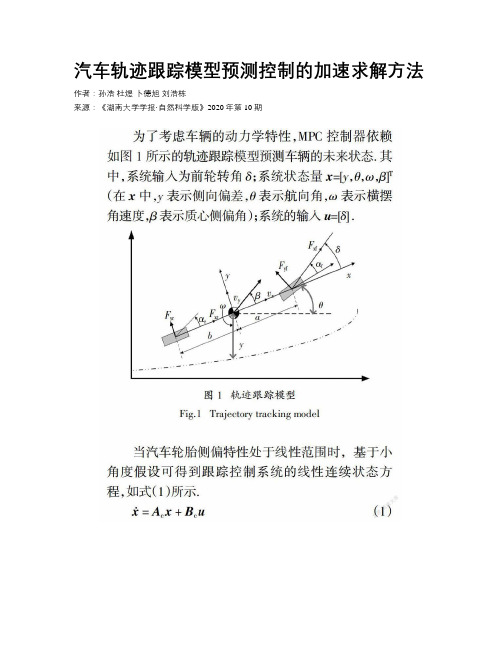
汽车轨迹跟踪模型预测控制的加速求解方法作者:孙浩杜煜卜德旭刘浩栋来源:《湖南大学学报·自然科学版》2020年第10期摘要:针对汽车轨迹跟踪模型预测控制求解中存在的规模较大、求解效率较低的问题,提出一种基于时域分解的加速计算方法提高求解效率. 首先引入全局一致性变量,将模型预测控制中邻接控制周期的时域耦合约束转化为全局一致性约束,实现时域解耦;随后在交叉方向乘子法框架下推导了时域分解后优化问题的分块更新方法,并设计了分块更新数值求解问题的停止准则,从而将大规模优化问题转化为小规模子问题;最后搭建了Simulink-CarSim平台进行了算法的仿真验证. 仿真结果表明,在求解精度不变的情况下,求解耗时下降24.21%,从而实现模型预测控制问题的加速求解.关键词:模型预测控制;自动驾驶汽车;轨迹跟踪;交叉方向乘子法;时域分解中图分类号:U461.99 文献标志码:AAccelerated Solution Method for Vehicle TrajectoryTracking Based on Model Predictive ControlSUN Hao1,2,DU Yu1,2†,BU Dexu3,LIU Haodong1,2(1. Beijing Key Laboratory of Information Service Engineering,Beijing Union University,Beijing 100101,China;2. College of Robotics,Beijing Union University,Beijing 100027,China;3. College of Traffic and Transportation Engineering,Central South University,Changsha 410076,China)Abstract:To solve the problems of large scale and low efficiency in the solution of intelligent vehicle trajectory tracking algorithm based on model predictive control,this paper proposes a time-domain splitting method to accelerate the calculation. First,global consistency variables are introduced to transform the time-domain coupling constraints of the adjacent control cycles into global consistency constraints,thus to achieve time-domain decoupling. Then,under the framework of Alternating Direction Method of Multipliers,the block updating method of optimization problem after time domain splitting is derived,and the stop criterion of block updating numerical solution is designed. Therefore,the large-scale optimization problem is converted into several small-scale sub-problems. Finally,the Simulink-CarSim platform is set up and the algorithm is verified by simulation. The simulation results show that,under the same accuracy of the solution,the efficiency of solution is improved by 24.21% on average with the proposed method,achieving accelerated solution for vehicle trajectory tracking based on model predictive control.Key words:model predictive control; autonomous vehicles; path tracking; alternating direction method of multipliers; time splitting自動驾驶汽车是提高交通系统安全、效率、经济等性能的有效途径,而轨迹跟踪是实现智能驾驶的核心技术之一[1],其目标是在满足汽车复杂动力学约束、行驶安全性约束前提下,以较小的偏差、较高的舒适性跟踪所规划的轨迹[2]. 模型预测控制(ModelPredictive Control,MPC)最早被应用在成本不敏感的大型工程中(如化工产业),并被认为是当年最具影响力的现代控制算法之一[3]. MPC通过引入参考模型,对约束的处理直接简单,不仅能够有效处理被控模型特性、约束带来影响,还能够通过滚动求解优化问题找到当前的最优控制量[4].基于上述优点,MPC在汽车轨迹跟踪问题的研究中得到国内外研究者的广泛关注.求解MPC问题的主流思路是将其转化为二次规划(Quadratic Programming,QP)问题. 其中,无约束MPC求解相对简单. Xu等以跟踪误差为性能指标实现AGV的轨迹跟踪控制[5],Shen等则建立了综合考虑跟踪精度和舒适性的目标函数[6],也有研究将输入量的边界建模为目标函数中代价值,构成“软约束”,但其数学原问题仍是无约束二次规划. 无约束二次规划问题可通过梯度下降等方法直接求解,但其局限在于仅考虑车辆的运动及动力学约束,没有考虑运动过程中所受到的其它约束,局限性较强. 因此,约束MPC更具备实际意义. 如Bo等建立了基于动力学的增量模型,考虑了执行机构的动力学特性约束[7]; Cai等则通过4自由度车辆模型加入车辆运动的侧翻约束,提高车辆跟踪控制的安全性[8]. 约束MPC的数学原问题是约束QP问题(MPC-QP问题),需要通过数值优化方法计算求解. 求解约束二次规划问题主要采用主动集法、内点法等方法,迭代次数较多. Wang和Boyd的研究表明,对于状态维数为m、控制输入维数为n、求解时域为T的MPC问题,状态转移形式及控制输入形式的MPC-QP问题求解的时间复杂度分别为O([T(n+m)]3)和O([Tn]3)[9]. 综上,虽然MPC在轨迹跟踪问题研究中得到广泛关注,但MPC-QP问题存在规模大、求解所需的浮点运算多、求解效率低的缺点,制约了MPC的性能. 因此,提高轨迹跟踪MPC问题的求解效率具有重要的意义.针对上述问题,本文提出一种加速求解方法以提高求解效率. 该方法通过交叉方向乘子法(Alternating Direction Method of Multipliers,ADMM)实现汽车轨迹跟踪问题的时域分解,将集中大规模的优化问题转为分块小规模优化问题,从而降低汽车轨迹跟踪MPC问题的时间复杂度,实现求解加速.1 模型预测控制问题的时域分解1.1 问题建模为了考虑车辆的动力学特性,MPC控制器依赖如图1所示的轨迹跟踪模型预测车辆的未来状态. 其中,系统输入为前轮转角δ;系统状态量x=[y,θ,ω,β]T(在x中,y表示侧向偏差,θ表示航向角,ω表示横摆角速度,β表示质心侧偏角);系统的输入u=[δ] .当汽车轮胎侧偏特性处于线性范围时,基于小角度假设可得到跟踪控制系统的线性连续状态方程,如式(1)所示.式(1)中各矩阵如式(2)所示. 其中,k1、k2分别为二自由度模型中车辆前、后轮等效侧偏刚度;a、b分别为二自由度模型中车辆直线到前、后轴的距离.那么,可得线性离散时间系统的狀态空间模型,如式(3)所示.x(k+1) = Ad x(k) + Bd u(k)(3)且连续与离散系统矩阵转换关系如式(4)所示,其中Ts为离散系统的采样时间.不失一般性,假设当前时刻系统状态为x0,根据离散系统的状态方程(3),在预测时域N内系统的输入与系统状态之间的转移关系如图 2所示,其中x∈Rm,u∈Rn.设离散时刻t下系统的参考状态为rt,那么综合考虑跟踪精度、舒适性的优化目标函数J 可用式(5)表示. 式中Q∈Rm × m、R∈Rn × n分别为状态变量、输入变量的权重对角矩阵.在轨迹跟踪问题中,代价函数越小越好. 对式(5)进行展开,轨迹跟踪的MPC问题可转化为如式(6)所示的约束二次规划问题. 在目标函数中,省略了不影响极值求解的常数项. 在约束条件中,(6a)表示汽车的动力学约束,(6b)表示不同时刻下状态变量及控制变量的可行域约束. 可以看出,虽然目标函数J在时域上解耦,但由于约束条件(6a)的存在(即t周期的终止状态为t+1周期的初始状态),并不能在求解过程中实现问题的分块解耦计算.1.2 时域分解为了实现问题的时域解耦,本文引入全局一致性变量,将汽车动力学带来的时域耦合约束转为全局一致性约束,从而实现问题的分块求解. 图 3为ADMM时域分解示意图.首先,以控制周期为单位对状态变量、控制变量进行分块表达. 对于所关注预测时域内的N个控制周期,按照次序给予编号1到N. 对于每个控制周期,该周期初始状态量、输入状态量和输出状态量可分别用x(t)t表达,其中上角标(t)表示为变量所属的分块编号,且块内变量之间的关系由汽车动力学特性决定,如式(7)所示:而块间关系由时域耦合约束决定,满足式(8):为解耦式(8)所示的时域耦合约束,引入全局一致性变量[z][~] = (z0,z1,…,zN)T ,并使x与z之间满足如式(9)所示的关系,其中:(9a)表示分块(t)的输入变量与zt-1的一致性约束;(9b)表示分块(t)的输出变量与zt的一致性约束.因此,联合式(7)~式(9),问题(6)可重写为如式(10)所示形式. 此时,邻接块之间不存在直接关系,其耦合约束通过一致性变量间接表达,从而实现控制周期之间时域解耦.2 分块求解方法2.1 问题求解综上所述,本文已经构建了MPC问题的时域分解范式,本节的工作则是基于ADMM求解时域分解后的问题. ADMM的标准构型如式(11)所示.为了方便地将式(10)转换为ADMM标准构型,引入块变量:[x][~]t = (x(t)求解MPC问题的主流思路是将其转化为二次规划(Quadratic Programming,QP)问题.其中,无约束MPC求解相对简单. Xu等以跟踪误差为性能指标实现AGV的轨迹跟踪控制[5],Shen等则建立了综合考虑跟踪精度和舒适性的目标函数[6],也有研究将输入量的边界建模为目标函数中代价值,构成“软约束”,但其数学原问题仍是无约束二次规划. 无约束二次规划问题可通过梯度下降等方法直接求解,但其局限在于仅考虑车辆的运动及动力学约束,没有考虑运动过程中所受到的其它约束,局限性较强. 因此,约束MPC更具备实际意义. 如Bo等建立了基于动力学的增量模型,考虑了执行机构的动力学特性约束[7]; Cai等则通过4自由度车辆模型加入车辆运动的侧翻约束,提高车辆跟踪控制的安全性[8]. 约束MPC的数学原问题是约束QP问题(MPC-QP问题),需要通过数值优化方法计算求解. 求解约束二次规划问题主要采用主动集法、内点法等方法,迭代次数较多. Wang和Boyd的研究表明,对于状态维数为m、控制输入维数为n、求解时域为T的MPC问题,状态转移形式及控制输入形式的MPC-QP问题求解的时间复杂度分别为O([T(n+m)]3)和O([Tn]3)[9]. 综上,虽然MPC在轨迹跟踪问题研究中得到广泛关注,但MPC-QP问题存在规模大、求解所需的浮点运算多、求解效率低的缺点,制约了MPC的性能. 因此,提高轨迹跟踪MPC问题的求解效率具有重要的意义.针对上述问题,本文提出一种加速求解方法以提高求解效率. 该方法通过交叉方向乘子法(Alternating Direction Method of Multipliers,ADMM)实现汽车轨迹跟踪问题的时域分解,将集中大规模的优化问题转为分块小规模优化问题,从而降低汽车轨迹跟踪MPC问题的时间复杂度,实现求解加速.1 模型预测控制问题的时域分解1.1 问题建模为了考虑车辆的动力学特性,MPC控制器依赖如图1所示的轨迹跟踪模型预测车辆的未来状态. 其中,系统输入为前轮转角δ;系统状态量x=[y,θ,ω,β]T(在x中,y表示侧向偏差,θ表示航向角,ω表示横摆角速度,β表示质心侧偏角);系统的输入u=[δ] .当汽车轮胎侧偏特性处于线性范围时,基于小角度假设可得到跟踪控制系统的线性连续状态方程,如式(1)所示.式(1)中各矩阵如式(2)所示. 其中,k1、k2分别为二自由度模型中车辆前、后轮等效侧偏刚度;a、b分别为二自由度模型中车辆直线到前、后轴的距离.那么,可得线性离散时间系统的状态空间模型,如式(3)所示.x(k+1) = Ad x(k) + Bd u(k)(3)且连续与离散系统矩阵转换关系如式(4)所示,其中Ts为离散系统的采样时间.不失一般性,假设当前时刻系统状态为x0,根据离散系统的状态方程(3),在预测时域N内系统的输入与系统状态之间的转移关系如图 2所示,其中x∈Rm,u∈Rn.設离散时刻t下系统的参考状态为rt,那么综合考虑跟踪精度、舒适性的优化目标函数J 可用式(5)表示. 式中Q∈Rm × m、R∈Rn × n分别为状态变量、输入变量的权重对角矩阵.在轨迹跟踪问题中,代价函数越小越好. 对式(5)进行展开,轨迹跟踪的MPC问题可转化为如式(6)所示的约束二次规划问题. 在目标函数中,省略了不影响极值求解的常数项. 在约束条件中,(6a)表示汽车的动力学约束,(6b)表示不同时刻下状态变量及控制变量的可行域约束. 可以看出,虽然目标函数J在时域上解耦,但由于约束条件(6a)的存在(即t周期的终止状态为t+1周期的初始状态),并不能在求解过程中实现问题的分块解耦计算.1.2 时域分解为了实现问题的时域解耦,本文引入全局一致性变量,将汽车动力学带来的时域耦合约束转为全局一致性约束,从而实现问题的分块求解. 图 3为ADMM时域分解示意图.首先,以控制周期为单位对状态变量、控制变量进行分块表达. 对于所关注预测时域内的N个控制周期,按照次序给予编号1到N. 对于每个控制周期,该周期初始状态量、输入状态量和输出状态量可分别用x(t)t表达,其中上角标(t)表示为变量所属的分块编号,且块内变量之间的关系由汽车动力学特性决定,如式(7)所示:而块间关系由时域耦合约束决定,满足式(8):为解耦式(8)所示的时域耦合约束,引入全局一致性变量[z][~] = (z0,z1,…,zN)T ,并使x与z之间满足如式(9)所示的关系,其中:(9a)表示分块(t)的输入变量与zt-1的一致性约束;(9b)表示分块(t)的输出变量与zt的一致性约束.因此,联合式(7)~式(9),问题(6)可重写为如式(10)所示形式. 此时,邻接块之间不存在直接关系,其耦合约束通过一致性变量间接表达,从而实现控制周期之间时域解耦.2 分块求解方法2.1 问题求解综上所述,本文已经构建了MPC问题的时域分解范式,本节的工作则是基于ADMM求解时域分解后的问题. ADMM的标准构型如式(11)所示.为了方便地将式(10)转换为ADMM标准构型,引入块变量:[x][~]t = (x(t)求解MPC问题的主流思路是将其转化为二次规划(Quadratic Programming,QP)问题.其中,无约束MPC求解相对简单. Xu等以跟踪误差为性能指标实现AGV的轨迹跟踪控制[5],Shen等则建立了综合考虑跟踪精度和舒适性的目标函数[6],也有研究将输入量的边界建模为目标函数中代价值,构成“软约束”,但其数学原问题仍是无约束二次规划. 无约束二次规划问题可通过梯度下降等方法直接求解,但其局限在于仅考虑车辆的运动及动力学约束,没有考虑运动过程中所受到的其它约束,局限性较强. 因此,约束MPC更具备实际意义. 如Bo等建立了基于动力学的增量模型,考虑了执行机构的动力学特性约束[7]; Cai等则通过4自由度车辆模型加入车辆运动的侧翻约束,提高车辆跟踪控制的安全性[8]. 约束MPC的数学原问题是约束QP问题(MPC-QP问题),需要通过数值优化方法计算求解. 求解约束二次规划问题主要采用主动集法、内点法等方法,迭代次數较多. Wang和Boyd的研究表明,对于状态维数为m、控制输入维数为n、求解时域为T的MPC问题,状态转移形式及控制输入形式的MPC-QP问题求解的时间复杂度分别为O([T(n+m)]3)和O([Tn]3)[9]. 综上,虽然MPC在轨迹跟踪问题研究中得到广泛关注,但MPC-QP问题存在规模大、求解所需的浮点运算多、求解效率低的缺点,制约了MPC的性能. 因此,提高轨迹跟踪MPC问题的求解效率具有重要的意义.针对上述问题,本文提出一种加速求解方法以提高求解效率. 该方法通过交叉方向乘子法(Alternating Direction Method of Multipliers,ADMM)实现汽车轨迹跟踪问题的时域分解,将集中大规模的优化问题转为分块小规模优化问题,从而降低汽车轨迹跟踪MPC问题的时间复杂度,实现求解加速.1 模型预测控制问题的时域分解1.1 问题建模为了考虑车辆的动力学特性,MPC控制器依赖如图1所示的轨迹跟踪模型预测车辆的未来状态. 其中,系统输入为前轮转角δ;系统状态量x=[y,θ,ω,β]T(在x中,y表示侧向偏差,θ表示航向角,ω表示横摆角速度,β表示质心侧偏角);系统的输入u=[δ] .当汽车轮胎侧偏特性处于线性范围时,基于小角度假设可得到跟踪控制系统的线性连续状态方程,如式(1)所示.式(1)中各矩阵如式(2)所示. 其中,k1、k2分别为二自由度模型中车辆前、后轮等效侧偏刚度;a、b分别为二自由度模型中车辆直线到前、后轴的距离.那么,可得线性离散时间系统的状态空间模型,如式(3)所示.x(k+1) = Ad x(k) + Bd u(k)(3)且连续与离散系统矩阵转换关系如式(4)所示,其中Ts为离散系统的采样时间.不失一般性,假设当前时刻系统状态为x0,根据离散系统的状态方程(3),在预测时域N内系统的输入与系统状态之间的转移关系如图 2所示,其中x∈Rm,u∈Rn.设离散时刻t下系统的参考状态为rt,那么综合考虑跟踪精度、舒适性的优化目标函数J 可用式(5)表示. 式中Q∈Rm × m、R∈Rn × n分别为状态变量、输入变量的权重对角矩阵.在轨迹跟踪问题中,代价函数越小越好. 对式(5)进行展开,轨迹跟踪的MPC问题可转化为如式(6)所示的约束二次规划问题. 在目标函数中,省略了不影响极值求解的常数项. 在约束条件中,(6a)表示汽车的动力学约束,(6b)表示不同时刻下状态变量及控制变量的可行域约束. 可以看出,虽然目标函数J在时域上解耦,但由于约束条件(6a)的存在(即t周期的终止状态为t+1周期的初始状态),并不能在求解过程中实现问题的分块解耦计算.1.2 时域分解为了实现问题的时域解耦,本文引入全局一致性变量,将汽车动力学带来的时域耦合约束转为全局一致性约束,从而实现问题的分块求解. 图 3为ADMM时域分解示意图.首先,以控制周期为单位对状态变量、控制变量进行分块表达. 对于所关注预测时域内的N个控制周期,按照次序给予编号1到N. 对于每个控制周期,该周期初始状态量、输入状态量和输出状态量可分别用x(t)t表达,其中上角标(t)表示为变量所属的分块编号,且块内变量之间的关系由汽车动力学特性决定,如式(7)所示:而块间关系由时域耦合约束决定,满足式(8):为解耦式(8)所示的时域耦合约束,引入全局一致性变量[z][~] = (z0,z1,…,zN)T ,并使x与z之间满足如式(9)所示的关系,其中:(9a)表示分块(t)的输入变量与zt-1的一致性约束;(9b)表示分块(t)的输出变量与zt的一致性约束.因此,联合式(7)~式(9),问题(6)可重写为如式(10)所示形式. 此时,邻接块之间不存在直接关系,其耦合约束通过一致性变量间接表达,从而实现控制周期之间时域解耦.2 分块求解方法2.1 问题求解综上所述,本文已经构建了MPC问题的时域分解范式,本节的工作则是基于ADMM求解时域分解后的问题. ADMM的标准构型如式(11)所示.为了方便地将式(10)转换为ADMM标准构型,引入块变量:[x][~]t = (x(t)。
基于二自由度模型的mpc在车辆横向控制中的应用

基于二自由度模型的mpc在车辆横向控制中的应用下载提示:该文档是本店铺精心编制而成的,希望大家下载后,能够帮助大家解决实际问题。
文档下载后可定制修改,请根据实际需要进行调整和使用,谢谢!本店铺为大家提供各种类型的实用资料,如教育随笔、日记赏析、句子摘抄、古诗大全、经典美文、话题作文、工作总结、词语解析、文案摘录、其他资料等等,想了解不同资料格式和写法,敬请关注!Download tips: This document is carefully compiled by this editor. I hope that after you download it, it can help you solve practical problems. The document can be customized and modified after downloading, please adjust and use it according to actual needs, thank you! In addition, this shop provides you with various types of practical materials, such as educational essays, diary appreciation, sentence excerpts, ancient poems, classic articles, topic composition, work summary, word parsing, copy excerpts, other materials and so on, want to know different data formats and writing methods, please pay attention!基于二自由度模型的MPC在车辆横向控制中的应用一、引言随着车辆自动驾驶技术的快速发展,车辆横向控制技术也变得愈发重要。
基于MPC的二阶倒立摆稳定控制

数值 0.4 0.2 0.2 0.5 0.5
假设摆的质心在连杆的几何中心,且为实心杆,
2
那么有
li
=
Li 2
,Ji
=
mLi 2
,(i=1,2)。
在理想(忽略所有
摩擦与干扰)的情况下,基于拉格朗日方程对系统
进行建模。 得拉格朗日方程为
"d #$ dt
La z觶 i
- La zi
=Fi,i=1,2,…,n
DOI:10.19557/ki.1001-9944.2022.09.004
控制系统与智能制造
基于 MPC 的二阶倒立摆稳定控制
石转转,郭开玺,张 品,张占东
(山西大同大学 机电工程学院,大同 037003)
摘要:倒立摆系统是一个典型的欠驱动、强耦合、非线性的机械系统,该文提出了利用模型
预测控制(MPC)方法来实现二阶倒立摆系统的稳定控制。 首先基于拉格朗日方程对二阶
θ2 m2
L2 l2
θ1
L 1 m 1 l1
x
F
m
图 1 机械式二阶倒立摆系统 Fig.1 Mechanical double inverted pendulum system
其中 F 是控制输入,表示水平拉力;θ1∈(-π,π) 表示摆杆 1(即下摆杆,链接在小车上)与竖直垂线 之 间 的 夹 角 ;θ2∈(-π,π)表 示 摆 杆 2(即 上 摆 杆 ,链 接在摆杆 1 的另一端)与竖直垂线之间的夹角。 此 外;m,m1 和 m2 分别代表小车、摆杆 1 和摆杆 2 的质 量;L1 和 L2 分别代表摆杆 1 和摆杆 2 的长度;l1 和 l2 分别表示摆杆 1 和摆杆 2 摆杆质心到低端的长 度 ;J1 和 J2 分 别表 示 摆 杆 1 和 摆 杆 2 的 转 动 惯 量 。 此外,二阶倒立摆系统的机械参数取值如表 1 所示, g 表示重力加速度,参数取自于文献[8]。
摄影专业词汇(中英文对照)

Power zoom电动变焦
Predictive 预测
Predictive focus control
预测焦点控制
Preflash预闪
Professional专业的
Program程序
Program back 程序机背
Program flash程序闪光
Phase detection相位检测
Photography摄影
Pincushion distortion枕形畸变
Plane of focus 焦点平面
Point of view视点
Polarizing偏振、偏光
Polarizer偏振镜
Portrait人像、肖像
Power 电源、功率、电动
Close-up 近摄
Coated镀膜
Compact camera 袖珍相机
Composition 构图
Compound lens 复合透镜
Computer计算机
Contact 触点
Continuous advance连续进片
Continuous autofocus连续自动聚焦
Rear curtain 后帘
Reciprocity failure 倒易律失效
Reciprocity Law 倒易律
Recompose 重新构图
Red eye红眼
Red eye reduction红眼减少
Reflector反射器、反光板
Reflex反光
Remote control terminal
可收缩TTL闪光灯
Second curtain后帘、第二帘幕
基于性能触发的双层结构模型预测控制

基于性能触发的双层结构模型预测控制王琳;邹媛媛;李少远【期刊名称】《上海交通大学学报》【年(卷),期】2018(0)10【摘要】双层控制结构广泛应用于工业过程控制,针对实际系统中不确定性导致的性能下降和控制不可行的问题,提出一种事件触发的动态实时优化(Dynamic Real-Time Optimization,D-RTO)与模型预测控制(Model Predictive Control,MPC)双层结构.上层采用经济模型预测控制(Economic MPC,EMPC)对目标函数进行优化,计算最优参考轨迹并传给下层;下层采用MPC使系统跟踪上层轨迹;通过构建基于性能指标的事件触发条件来及时补偿不确定性造成的系统性能损失,无需等到D-RTO的下一次优化.当实际系统性能指标与上层优化的性能指标之差超出阈值时,需要重新求解EMPC,并基于当前状态更新参考轨迹.在此基础上,进一步分析了事件触发的D-RTO与MPC双层控制结构的可行性和闭环稳定性.数值模拟实验验证了方法的有效性.【总页数】9页(P1324-1332)【关键词】模型预测控制;双层控制结构;动态实时优化;事件触发;不确定性【作者】王琳;邹媛媛;李少远【作者单位】上海交通大学自动化系;系统控制与信息处理教育部重点实验室【正文语种】中文【中图分类】TP273【相关文献】1.基于多模型广义预测控制器的DRTO双层结构 [J], 宋治强;王昕;王振雷2.双层结构模型预测控制算法性能分析 [J], 孙浩杰;邹涛;李丽娟3.基于累积平方误差–总平方波动指标的模型预测控制器性能评价及自愈 [J], 张浩;赵众4.基于模型预测控制的电动汽车起步工况仿真与性能评价 [J], 李文礼;陆宇;汪杨凡;郑维东;严海燕;徐瑞5.基于模型预测控制的电动汽车起步工况仿真与性能评价 [J], 李文礼;陆宇;汪杨凡;郑维东;严海燕;徐瑞因版权原因,仅展示原文概要,查看原文内容请购买。
切削力波形的数字滤波研究_杨俊茹

High Speed Machining .Annals of the CIRP , 1994.43 (1): 363~ 366
Abstract :Cutting fore measurement is very important during the cutting process.The collected cutting force signal is not often perfect
due to outside interfere and condition limition .This paper proposes to use digital filter to solve the problem , and the design of a digital filter
山东省自然科学基金会和国家教委留学回国人员基金资助课 题
· 48 ·
2 滤波结果 图 2 和图 3 分别表示了滤波前和滤波后 的切削力
波形 , 比较这两个图 , 可以看出 , 滤波前采集到的切 削力信号比较乱 , 经过本文设计的数字滤波器滤波之
图 2 滤波前切削力的波形
图 3 滤波后切削力的波形
的切削力信号进行了比较 , 结果表明效果很好 。
参考文献
【1】 葛 革 , 艾 兴 .评价断续 车削淬 硬钢时 硬质合 金刀 具抗早期破损能力的一 个参数 .机械 工程学报 , 1983 . 192 (6)
【2】 陈献延编著 .硬质合 金使用手 册 .北京 :冶金工 业出 版社 , 1986
- 1、下载文档前请自行甄别文档内容的完整性,平台不提供额外的编辑、内容补充、找答案等附加服务。
- 2、"仅部分预览"的文档,不可在线预览部分如存在完整性等问题,可反馈申请退款(可完整预览的文档不适用该条件!)。
- 3、如文档侵犯您的权益,请联系客服反馈,我们会尽快为您处理(人工客服工作时间:9:00-18:30)。
Cross-coupled Model Predictive Control for Multi-axis Coordinated MotionSystemsXu Zhang1, 2, Kuanyi Zhu2, Xueyou Yang11. College of Precision Instrument and Optoelectronics Engineering, Tianjin University,Tianjin 300072, ChinaE-mail: redheartzx@2. School of Electrical and Electronic Engineering, Nanyang Technological University,Singapore 639798, SingaporeAbstractA cross-coupled model predictive controller for multi-axis coordinated motion systems is presented by incorporating cross-coupled strategy into the model predictive control architecture. The control law is generated by minimizing a cost function for the augmented system model in which the synchronization errors are embedded. Simulation and experimental results conducted on a high-precision positioning system with two permanent magnet linear motors (PMLMs) demonstrate the effectiveness of the proposed approach.1.IntroductionHigh-precision multi-axis motion systems are essential elements in modern advanced manufacturing. The term “axis of motion” refers to one degree of freedom, or forward and backward motion along one direction, which may be linear or rotary motion. When two or more axes of motion are involved on a single machine, that machine is employing multi-axis motion. In precision motion control, besides good tracking performance of each individual axis is absolutely necessary, synchronization or coordination between multiple axes becomes another challenging problem needed to be solved [1].Demand for high-precision control of multi-axis motion systems calls for the development of high performance positioning devices and accompanying control approaches. With the attractive features such as high dynamic performance and most importantly high positioning precision, permanent magnet linear motors (PM LM s) are increasingly widely being applied in multi-axis motion systems [2]. To harness the potential of PM LM s, the main challenge lies in the control approach.Cross-coupled control is an appropriate strategy used for coordinated control of processes with multiple motion axes. This concept has been successfully applied to reducing contour error of multiple motion axes in machine tool control [3]–[6], minimizing differential velocity error of two driving wheels in a mobile vehicle [7], and synchronizing the multi-robot for assembly tasks respectively [8]. However, the principal shortcoming of the existing control techniques is that they cannot explicitly incorporate plant model uncertainties in the formulation of the high precision control system when using the traditional PID or fussy method.M odel predictive control (M PC) algorithm is an effective approach to improve motion tracking and coordination performance of multi-axis systems due to its control acumen to deal with the multivariable constrained control problems. In the past two decades, the theory of MPC has been well developed nearly in all aspects, such as stability, nonlinearity, and robustness [9]–[13]. Several methods based on M PC are presented for better positioning and tracking precision of a single axis or motor [14]–[17]. A cross-coupling framework of generalized predictive control is investigated by compensating both tracking error and synchronous error between the process and the reference model [18]. In this paper, design and implementation of a cross-coupled model predictive control algorithm are presented for multi-axis motion systems. This paper is organized as follows. In Section 2, the dynamics of the PM LM is presented. Process model and MPC is formulated in Section 3. In Section 4, synchronization strategy is proposed. The cross coupled M PC controller for multi-axis coordinated motion systems is presented in Section 5. Simulations and experiments are performed in Section 6, and finally, conclusions are given in Section 7.International Conference on Advanced Computer Control2. Dynamics of the PMLMThe dynamics of the PM LM can be viewed as comprising of a dominantly linear model and a nonlinear remnant [19]. In the dominant linear model, the mechanical and electrical dynamics of a PM LM can be expressed as follows:d m MxDx F F ++= (1) ()ae a a a dI K xL R I u t dt++= (2)m f a F K I = (3)where x(t) denotes motor position; M ,D ,F m , and F d denote mechanical parameters, i.e., mass of the moving thrust block, viscosity constant, generated force, and system disturbance, respectively; u(t),I a ,R a , and L a denote electrical parameters, i.e., time-varying motor terminal voltage, armature current, armature resistance, and armature inductance, respectively; K f denotes an electrical–mechanical energy conversion constant; and K e is back electromotive force (EM F) voltage. The delay due to electrical transient response may be ignored since the electrical time constant is typically much smaller than the mechanical one. The following is the simplified model:()()()x axt bu t t ξ=++ (4) wheref e a K K R D a RM+=−fa Kb R M =()dF t M ξ=−.Note that Ӷ(t) includes extraneous nonlinear effectsthat may be present in the physical structure. Among them, the prominent nonlinear effect is due to ripple force arising from the magnetic structure of the PMLM and other physical imperfections, which can be viewed as a sinusoidal function of motor position with a period of Ԁ and amplitudes of A r and B r , i.e.,cos()sin()ripple r r F A x B x ωω=+ (5)where F ripple is ripple force. In particular, ripple force ismore complex in shape, e.g., due to variations in the magnet dimension.3. Process model and MPCA process with multiple PM LM s can be describedby the linear discrete-time CARIMA model:111()()()(1)()()/i i i i i i A q x t B q u t C q t ξ−−−=−+Δ(6)where t is the normalized discrete time, i denotes the corresponding motor of the process, x i (t) and u i (t) are the position and control input of the motor, respectively, Ӷi (k) represents system disturbance andunmodeled dynamics, A i (q -1)and B i (q -1) are the systempolynomials in the backward shift operator q -1,C i (q -1) is a polynomial used for robustness of the controller, and Ӕ is the differencing operator.In model predictive control, minimization of a cost function yields the control law. The cost function is:211{(()(|))Hpn c i i i k I w t k x t k t ===+−+¦¦,21((1|)}Hci i i k u t k t λ=+Δ+−¦ (7)where w i (t + k) is the reference signal, H p and H c are the prediction and control horizons, respectively, ӳi is a non-negative weighing factor for the control input. Based on MPC technique, the future output x i (t + k|t)can be expressed as(|)(1|)()i i ik ik x t k t G u t k t p t +=+−+,1,2,3,......,p k N = (8)where11k ik ik ik G G g q −+−=+ (9)()()(1)i ik ik ik i iiF H p t x t u t C C =+Δ− (10)G ik , F ik and H ik satisfy the Diophantine equationsk i i ik ik C A E q F −=Δ+ (11) k i ik i ik ik B E C G q H −=+ (12)with the corresponding degrees() () 1() max((), ())() max((), ())1ik ik iki i ik i i E G k F A C k H B C δδδδδδδδ==−=−=−°®°¯(13) The matrix version of the predictor (8) is obtained asi i i i X G U P =+ (14)where[( 1|) ( 2|) ... ( |)]T i i i i p X x t t x t t x t N t =+++ (15) [( |) ( 1|) ... ( 1|)]T i i i i u U u t t u t t u t N t =ΔΔ+Δ+− (16)12 [() () ... ()]p N T i i i i P p t p t p t = (17)0100(1)(2)(1)(2)()000u u p p p u i i i i N i N i i N i N i N N i g g g G g g g g g g −−−−−…=…ªº«»«»«»«»«»«»«»«»¬¼%##%%%#%%# (18)4. Synchronization strategyIn multi-axis coordinated motion systems, both tracking performance and synchronization performance are specified. However, if the motors follow different trajectories, i.e., r i (t) r j (t), then a scalar of r i (t)/r j (t) should be introduced to describe the relationship between the ith motor and the jth motor accurately. So the synchronization error can be defined as() (() ()) ij ij i ij j t x t x t φαβ=− (19) where өij and Ӫij are the coupling and synchronizationfactors between the ith motor and the jth motor, respectively. M oreover, even if Ĩij (t) = 0 may be achieved at an instant time, the overall system may not be synchronized perfectly due to ӔĨij (t + 1) 0,where ӔĨij (t + 1) = Ĩij (t + 1) íĨij (t). In this case, the difference between the consecutive synchronization errors should also be considered as1() (1 )()ij ij t q t ψφ−=− (20)denoting[( 1|) ( 2|) ... ( |)]T ij ij ij ij p t t t t t N t φφφΦ=+++ (21) [( 1|) ( 2|) ... ( |)]T ij ij ij ij p t t t t t N t ψψψΨ=+++ (22)For the synchronization error and its difference, bysetting ӿij(t + 1|t) = 0,it can be obtained thatij ij L Ψ=Φ (23)where00001100011100011L −=−−−ªº«»«»«»«»«»«»¬¼""%##%%" (24)The cost function is introduced as1{()()}i i i i i i i nT T c i W X W X U U I λ=−−+=¦111n nij ij i j i T −==++ΦΦ¦¦ȁ (25)where[( 1) ( 2) ... ( )]T i i i i p W w t w t w t N =+++ (26)TI L L υη=+ȁ (27)and I is the unit matrix.5. Cross-coupled MPC controllerBy minimizing the cost function (25), the Cross-coupled MPC control law can be obtained:()()21111122122222312n m m m m n m m m m n n n W P P P U U W P P P U W P αβαβ=−==ΩΓ§ªº−−Λ−ªº¨«»«»¨«»−−Λ−«»¨«»«»¨«»«»¨«»¨¬¼−¬¼©¦¦##()()12222211210m m m m m n mn mn mmn n m P P P P αββαββ=−=·ªº¸«»Λ−¸«»+¸«»¸«»¸«»¸Λ−¬¼¹¦¦# (28)where Ө,ӓ,Өij are expressed as follows1111n n nn ΩΩΩ=ΩΩªº«»«»«»¬¼"#%#" (29)100T Tn G G Γ=ªº«»«»«»¬¼"#%#" (30)2, ,Ti i ij Tij ij j i i G G I if i jG G if i j λαρΟ+=ΩΛ<°=®−°¯ (31) 122211()i nmi mi im m m i I αβα−==+Ο=+Λ+¦¦ (32)The block diagram shown in Figure 1 illustrates thestructure of cross-coupled MPC controller.Figure 1. Structure of cross-coupled MPCcontroller6. Simulation and experimentFigure 2. High-precision positioning controlsystemThe effectiveness of the proposed control approach will be illustrated by computer simulations and experiments on a high-precision positioning system with two PMLMs, as shown in Figure 2. The dynamics of the positioning system can be described by11120.653()11.006()x xt u t =−+ ()11.418sin 20.074x π+ ()10.313cos 20.074x π− (33)2225.917() 5.048()x xt u t =−+ ()20.676sin 20.051x π+ ()2cos 0.19120.051x π− (34)With a sampling interval T s = 0.0008 seconds, the corresponding linear discrete-time system models are given by111()() ()(1) ()/(1),i i i i i i A q x t B q u t C t q ξ−−−=−+− 1, 2i = (35)where11211122111112112() 1.000 1.9840.984() 1.000 1.9950.995() 3.502 3.483() 1.613 1.610 10.8,,,,.A q q q A q q qB q q B q qC C q −−−−−−−−−−−=−+=−+=−=−==−In this study, two PM LM s are desired to track thesame square wave. The parameters of the cross-coupled M PC controller are set as: N p = 10; N c = 4; ӳ=50,ӵ = 20,ӯ = 10,ө12 = 1,Ӫ12 = 1. Figure 3-5 show the desired tracking trajectories of two PMLMs, the simulation and experimental results for the cross-coupled MPC controller, respectively.Figure 3. Desired tracking trajectoriesFigure 4. Simulation results for the cross-coupled MPC controllerFigure 5. Experimental results for the cross-coupled MPC controller7. ConclusionTo achieve better synchronization performance while maintaining good tracking response, a cross-coupled M PC controller for multi-axis coordinated motion systems has been presented. Computer simulations and experiments on a high-precision positioning system with two PMLMs have shown that the improved performance of the control system can be obtained with the control parameters to be set as follows: first, N p ,N c and ӳare selected appropriately so that the control system provides a stable andsatisfactory tracking response and then, the weighting factorsӵandӯare introduced to reduce the synchronization errors caused by the mismatched dynamics, system disturbances, and so on. Although the same desired trajectory is considered in this study, different trajectories can be realized easily by setting the synchronization factorsөand Ӫʳappropriately.8. References[1] T.C. Chiu and M. Tomizuka, “Coordinated position control of multi-axis mechanical system”, Trans. ASME, J. Dyn. Syst. Meas. Control, 1998, vol. 120, no.3, pp.389–393. [2] K.K. Tan, T.H. Lee, H.F. Dou, and S.N. Huang, Precision Motion Control: Design and Implementation (Advances in Industrial Control). London, U.K.: Springer-Verlag, 2001.[3] J. Borenstein and Y. Koren, “Motion control analysis ofa mobile robot”, Trans. ASME, J. Dyn. Syst. Meas. Control, Jun. 1987, vol. 109, no. 2, pp. 73–79.[4] Y. Koren and C.C. Lo, “Variable-gain cross-coupling controller for contouring,” Ann. CIRP, 1991, vol. 40, no. 1, pp. 371–374.[5] S.S. Yeh and P.L. Hsu, “Analysis and design of integrated control for multi-axis motion systems” , IEEE Trans. Control Syst. Technol., May 2003, vol. 11, no. 3, pp. 375–382.[6] P.K. Kulkarni and K. Srinivasan, “Cross-coupled control of biaxial feed drive servomechanisms”, Trans. ASME, J. Dyn. Syst. Meas. Control, 1990, vol. 112, no. 2, pp. 225–232.[7] L. Feng, Y. Koren, and J. Borenstein, “Cross-coupling motion controller for mobile robots,” IEEE Control Syst. Mag., Dec. 1993, vol. 13, no. 6, pp. 35–43.[8] D. Sun and J.K. M ills, “Adaptive synchronized control for coordination of multirobot assembly tasks,” IEEE Trans. Robot. Autom., Aug. 2002, vol. 18, no. 4, pp. 498–510. [9] D. W. Clarke, C. Mohtadi, and P. S. Tuffs, “Generalized predictive control—Part I. The basic algorithm,” Automatica, Mar. 1987, vol. 23, no. 2, pp. 137–148.[10]D. W. Clarke, C. Mohtadi, and P. S. Tuffs, “Generalized predictive control—Part II. Extensions and interpretations,” Automatica, Mar. 1987, vol. 23, no. 2, pp. 149–160.[11] M. Morari and J. H. Lee, “Model predictive control: Past, present and future,” Comput. Chem. Eng., 1999, vol. 23, no. 4/5, pp. 667–682.[12] D. Q. Mayne, J. B. Rawlings, C. V. Rao, and P. O. M. Scokaert, “Constrained model predictive control: Stability and optimality,” Automatica, Jun. 2000, vol. 36, no. 6, pp. 789–814.[13] J. M. M aciejowski, Predictive Control: With Constraints. London, U.K.: Prentice-Hall, 2002.[14] L. Zhang, H.R. Norman, and W. Shepherd, “Long range predictive control of a current regulated PWM for induction drives using the synchronous reference frame,” IEEE Trans. Control Syst. Technol., Jan. 1997, vol. 5, pp. 119–126.[15] K.S. Low, K.Y. Chiun, and K.V. Ling, “Evaluating Generalized Predictive Control for a Brushless dc Drive,” IEEE Trans. Power Electron., Nov. 1998, vol. 13, pp. 1191–1198.[16] K. Hentabli, M.E.H. Benbouzid, and D. Pinchon, “M ultivariable state-space CGPC application to induction motor control,” in Proc IECON’97, 1997, vol. 1, pp. 181–186.[17] M. Kinnaert, “Adaptive generalized predictive controller for MIMO systems,” Int. J. Control, 1989, vol. 50, no. 1, pp. 161–172.[18] K.Y. Zhu and B.P. Chen, “Cross-coupling design of generalized predictive control with reference models,” in Proc. Inst. Mech. Eng., 2001, vol. 215, pt. I, no. 4, pp. 375–384.。