VibroMatrix_1.6_Manual

合集下载

Autodesk Nastran 2023 参考手册说明书

DATINFILE1 ........................................................................................................................................................... 9
FILESPEC ............................................................................................................................................................ 13
DISPFILE ............................................................................................................................................................. 11
File Management Directives – Output File Specifications: .............................................................................. 5
BULKDATAFILE .................................................................................................................................................... 7

ClusVis 1.2.0 用户手册说明书

Package‘ClusVis’October12,2022Type PackageTitle Gaussian-Based Visualization of Gaussian and Non-GaussianModel-Based ClusteringVersion1.2.0Author Christophe Biernacki[aut],Matthieu Marbac[aut,cre],Vincent Vandewalle[aut]Maintainer Matthieu Marbac<*************************>Description Gaussian-Based Visualization of Gaussian and Non-Gaussian Model-Based Cluster-ing done on any type of data.Visualization is based on the probabilities of classiﬁcation. License GPL(>=2)Imports Rcpp,MASS,parallel,mgcv,mvtnorm,Rmixmod,VarSelLCM(>=2.1)LinkingTo Rcpp,RcppArmadillo,mvtnormByteCompile trueEncoding UTF-8LazyLoad yesLazyData trueCollate'clusvis.R''estimation.R''smartinit.R''RcppExports.R''plot.R''clusvismixmod.R''clusvisvarsellcm.R''modessearch.R'Depends R(>=3.4)RoxygenNote6.1.1NeedsCompilation yesRepository CRANDate/Publication2019-06-2408:30:15UTCR topics documented:ClusVis-package (2)clusvis (4)1clusvisMixmod (6)clusvisVarSelLCM (8)congress (9)plotDensityClusVisu (10)Index12 ClusVis-package Gaussian-Based Visualization of Gaussian and Non-Gaussian Model-Based Clustering.DescriptionThe main function for parameter inference is clusvis.Moreover,speciﬁc functions clusvisVarSelLCM and clusvisMixmod are implemented to visualize the results of the R package VarSelLCM and Rmixmod.After parameter inference,visualization is done with function plotDensityClusVisu. DetailsPackage:ClusVisType:PackageVersion: 1.1.0Date:2018-04-18License:GPL-3LazyLoad:yesAuthor(s)Biernacki,C.and Marbac,M.and Vandewalle,V.Examples##Not run:##First example:R package Rmixmod#Package loadingrequire(Rmixmod)#Data loading(categorical data)data("congress")#Model-based clustering with4componentsset.seed(123)res<-mixmodCluster(congress[,-1],4,strategy=mixmodStrategy(nbTryInInit=500,nbTry=25))#Inference of the parameters used for results visualization#(specific for Rmixmod results)#It is better because probabilities of classification are generated#by using the model parametersresvisu<-clusvisMixmod(res)#Component interpretation graphplotDensityClusVisu(resvisu)#Scatter-plot of the observation membershipsplotDensityClusVisu(resvisu,add.obs=TRUE)##Second example:R package Rmixmod#Package loadingrequire(Rmixmod)#Data loading(categorical data)data(birds)#Model-based clustering with3componentsresmixmod<-mixmodCluster(birds,3)#Inference of the parameters used for results visualization(general approach) #Probabilities of classification are not sampled from the model parameter,#but observed probabilities of classification are used for parameter estimation resvisu<-clusvis(log(resmixmod@bestResult@proba),resmixmod@bestResult@parameters@proportions)#Inference of the parameters used for results visualization#(specific for Rmixmod results)#It is better because probabilities of classification are generated#by using the model parametersresvisu<-clusvisMixmod(resmixmod)#Component interpretation graphplotDensityClusVisu(resvisu)#Scatter-plot of the observation membershipsplotDensityClusVisu(resvisu,add.obs=TRUE)##Third example:R package VarSelLCM#Package loadingrequire(VarSelLCM)#Data loading(categorical data)data("heart")#Model-based clustering with3componentsres<-VarSelCluster(heart[,-13],3)#Inference of the parameters used for results visualization#(specific for VarSelLCM results)#It is better because probabilities of classification are generated#by using the model parametersresvisu<-clusvisVarSelLCM(res)#Component interpretation graphplotDensityClusVisu(resvisu)#Scatter-plot of the observation membershipsplotDensityClusVisu(resvisu,add.obs=TRUE)##End(Not run)clusvis This function estimates the parameters used for visualizationDescriptionThis function estimates the parameters used for visualizationUsageclusvis(logtik.estim,prop=rep(1/ncol(logtik.estim),ncol(logtik.estim)),logtik.obs=NULL,maxit=10^3,nbrandomInit=12,nbcpu=1)Argumentslogtik.estim matrix.It contains the probabilities of classiﬁcation used for parameter infer-ence(should be sampled from the model parameter or computed from the ob-servations).prop vector.It contains the class proportions(by default,classes have same propor-tion).logtik.obs matrix.It contains the probabilities of classiﬁcation of the clustered sample.If missing,logtik.estim is used.maxit numeric.It limits the number of iterations for the Quasi-Newton algorithm(de-fault1000).nbrandomInit numeric.It deﬁnes the number of random initialization of the Quasi-Newton algorithm.nbcpu numeric.It speciﬁes the number of CPU(only for linux)ValueReturns a listExamples##Not run:##First example:R package Rmixmod#Package loadingrequire(Rmixmod)#Data loading(categorical data)data("congress")#Model-based clustering with4componentsset.seed(123)res<-mixmodCluster(congress[,-1],4,strategy=mixmodStrategy(nbTryInInit=500,nbTry=25)) #Inference of the parameters used for results visualization#(specific for Rmixmod results)#It is better because probabilities of classification are generated#by using the model parametersresvisu<-clusvisMixmod(res)#Component interpretation graphplotDensityClusVisu(resvisu)#Scatter-plot of the observation membershipsplotDensityClusVisu(resvisu,add.obs=TRUE)##Second example:R package Rmixmod#Package loadingrequire(Rmixmod)#Data loading(categorical data)data(birds)#Model-based clustering with3componentsresmixmod<-mixmodCluster(birds,3)#Inference of the parameters used for results visualization(general approach)#Probabilities of classification are not sampled from the model parameter,#but observed probabilities of classification are used for parameter estimationresvisu<-clusvis(log(resmixmod@bestResult@proba),resmixmod@bestResult@parameters@proportions)#Inference of the parameters used for results visualization#(specific for Rmixmod results)#It is better because probabilities of classification are generated#by using the model parametersresvisu<-clusvisMixmod(resmixmod)#Component interpretation graphplotDensityClusVisu(resvisu)#Scatter-plot of the observation membershipsplotDensityClusVisu(resvisu,add.obs=TRUE)##Third example:R package VarSelLCM#Package loadingrequire(VarSelLCM)#Data loading(categorical data)data("heart")#Model-based clustering with3componentsres<-VarSelCluster(heart[,-13],3)#Inference of the parameters used for results visualization#(specific for VarSelLCM results)#It is better because probabilities of classification are generated#by using the model parametersresvisu<-clusvisVarSelLCM(res)#Component interpretation graphplotDensityClusVisu(resvisu)#Scatter-plot of the observation membershipsplotDensityClusVisu(resvisu,add.obs=TRUE)##End(Not run)clusvisMixmod This function estimates the parameters used for visualization of model-based clustering performs with R package Rmixmod.To achieve theparameter infernece,it automatically samples probabilities of classi-ﬁcation from the model parametersDescriptionThis function estimates the parameters used for visualization of model-based clustering performs with R package Rmixmod.To achieve the parameter infernece,it automatically samples probabili-ties of classiﬁcation from the model parametersUsageclusvisMixmod(mixmodResult,sample.size=5000,maxit=10^3,nbrandomInit=4*mixmodResult@bestResult@nbCluster,nbcpu=1,loccont=NULL)ArgumentsmixmodResult[MixmodCluster]It is an instance of class MixmodCluster returned by function mixmodCluster of R package Rmixmod.sample.size numeric.Number of probabilities of classiﬁcation sampled for parameter infer-ence.maxit numeric.It limits the number of iterations for the Quasi-Newton algorithm(de-fault1000).nbrandomInit numeric.It deﬁnes the number of random initialization of the Quasi-Newtonalgorithm.nbcpu numeric.It speciﬁes the number of CPU(only for linux).loccont numeric.Index of the column containing continuous variables(only for mixed-type data).ValueReturns a listExamples##Not run:##First example:R package Rmixmod#Package loadingrequire(Rmixmod)#Data loading(categorical data)data("congress")#Model-based clustering with4componentsset.seed(123)res<-mixmodCluster(congress[,-1],4,strategy=mixmodStrategy(nbTryInInit=500,nbTry=25)) #Inference of the parameters used for results visualization#(specific for Rmixmod results)#It is better because probabilities of classification are generated#by using the model parametersresvisu<-clusvisMixmod(res)#Component interpretation graphplotDensityClusVisu(resvisu)#Scatter-plot of the observation membershipsplotDensityClusVisu(resvisu,add.obs=TRUE)##Second example:R package Rmixmod#Package loadingrequire(Rmixmod)#Data loading(categorical data)data(birds)#Model-based clustering with3componentsresmixmod<-mixmodCluster(birds,3)#Inference of the parameters used for results visualization(general approach)#Probabilities of classification are not sampled from the model parameter,8clusvisVarSelLCM #but observed probabilities of classification are used for parameter estimationresvisu<-clusvis(log(resmixmod@bestResult@proba),resmixmod@bestResult@parameters@proportions)#Inference of the parameters used for results visualization#(specific for Rmixmod results)#It is better because probabilities of classification are generated#by using the model parametersresvisu<-clusvisMixmod(resmixmod)#Component interpretation graphplotDensityClusVisu(resvisu)#Scatter-plot of the observation membershipsplotDensityClusVisu(resvisu,add.obs=TRUE)##End(Not run)clusvisVarSelLCM This function estimates the parameters used for visualization of model-based clustering performs with R package Rmixmod.To achieve theparameter infernece,it automatically samples probabilities of classi-ﬁcation from the model parametersDescriptionThis function estimates the parameters used for visualization of model-based clustering performs with R package Rmixmod.To achieve the parameter infernece,it automatically samples probabili-ties of classiﬁcation from the model parametersUsageclusvisVarSelLCM(varselResult,sample.size=5000,maxit=10^3,nbrandomInit=4*varselResult@model@g,nbcpu=1,loccont=NULL) ArgumentsvarselResult[VSLCMresults]It is an instance of class VSLCMresults returned by function VarSelCluster of R package VarSelLCM.sample.size numeric.Number of probabilities of classiﬁcation sampled for parameter infer-ence.maxit numeric.It limits the number of iterations for the Quasi-Newton algorithm(de-fault1000).nbrandomInit numeric.It deﬁnes the number of random initialization of the Quasi-Newton algorithm.nbcpu numeric.It speciﬁes the number of CPU(only for linux).loccont numeric.Index of the column containing continuous variables(only for mixed-type data).congress9ValueReturns a listExamples##Not run:#Package loadingrequire(VarSelLCM)#Data loading(categorical data)data("heart")#Model-based clustering with3componentsres<-VarSelCluster(heart[,-13],3)#Inference of the parameters used for results visualization#(specific for VarSelLCM results)#It is better because probabilities of classification are generated#by using the model parametersresvisu<-clusvisVarSelLCM(res)#Component interpretation graphplotDensityClusVisu(resvisu)#Scatter-plot of the observation membershipsplotDensityClusVisu(resvisu,add.obs=TRUE)##End(Not run)congress Real categorical data set:Congressional Voting Records Data SetDescriptionThis data set includes votes for each of the U.S.House of Representatives Congressmen on the16 key votes identiﬁed by the CQA.The CQA lists nine different types of votes:voted for,paired for,and announced for(these three simpliﬁed to yea),voted against,paired against,and announced against(these three simpliﬁed to nay),voted present,voted present to avoid conﬂict of interest,and did not vote or otherwise make a position known(these three simpliﬁed to an unknown disposition). ReferencesCongressional Quarterly Almanac,98th Congress,2nd session1984,V olume XL:Congressional Quarterly Inc.Washington,D.C.,1985.Schlimmer,J.C.(1987).Concept acquisition through representational adjustment.Doctoral disser-tation,Department of Information and Computer Science,University of California,Irvine,CA.Website:https:///ml/datasets/congressional+voting+records10plotDensityClusVisuExamplesdata(congress)plotDensityClusVisu Function for visualizing the clustering resultsDescriptionFunction for visualizing the clustering resultsUsageplotDensityClusVisu(res,dim=c(1,2),threshold=0.95,add.obs=FALSE,positionlegend="topright",xlim=NULL,ylim=NULL,colset=c("darkorange1","dodgerblue2","black","chartreuse2","darkorchid2","gold2","deeppink2","deepskyblue1","firebrick2","cyan1","red","yellow"))Argumentsres object return by function clusvis or clusvisdim numeric.This vector of size two choose the axes to represent.threshold numeric.It contains the thersholds used for computing the level curves.add.obs boolean.If TRUE,coordinnates of the observations are plotted.positionlegend character.It speciﬁes the legend location.xlim numeric.It speciﬁes the range of x-axis.ylim numeric.It speciﬁes the range of y-axis.colset character.It speciﬁes the colors of the observations per class.Examples##Not run:#Package loadingrequire(Rmixmod)#Data loading(categorical data)data("congress")#Model-based clustering with4componentsset.seed(123)res<-mixmodCluster(congress[,-1],4,strategy=mixmodStrategy(nbTryInInit=500,nbTry=25))#Inference of the parameters used for results visualization#(specific for Rmixmod results)#It is better because probabilities of classification are generated#by using the model parametersresvisu<-clusvisMixmod(res)plotDensityClusVisu11 #Component interpretation graphplotDensityClusVisu(resvisu)#Scatter-plot of the observation membershipsplotDensityClusVisu(resvisu,add.obs=TRUE)##End(Not run)Index∗datasetscongress,9∗packageClusVis-package,2ClusVis(ClusVis-package),2clusvis,2,4,10ClusVis-package,2clusvisMixmod,2,6clusvisVarSelLCM,2,8congress,9MixmodCluster,6plotDensityClusVisu,2,10VSLCMresults,812。

Datalogic Matrix 120 快速参考指南说明书

During the reader startup (reset or restart phase), all the LEDs blink for one second.
The single push button gives immediate access to the following relevant functions:
For quick access, from the home page click on the search icon
, and type
in the name of the product you’re looking for. This allows you access to
download Data Sheets, Manuals, Software & Utilities, and Drawings.
NPN/Open Collector
PNP/Open Emitter
NPN and PNP Output Wiring to CBX
I/O Using CAB-1051:
CAUTION: If output devices are powered externally (separate from Matrix 120 power), it is always advised to maintain the same voltage levels used for the Matrix 120 device.
Hover over the Support & Service menu for access to Services and Technical Support.
INSTALLATION PROCEDURE

蓝眼 Matrix 矩阵控制软件使用手册说明书

在使用本产品之前，请务必先仔细阅读本使用说明书。

请务必妥善保管好本书，以便日后能随时查阅。

请在充分理解内容的基础上，正确使用。

【爱护地球，蓝眼用心】本手册采用环保打印，如需电子文件请向代理商或蓝眼科技客服中心免费索取。

矩阵控制软件使用手册Version 1.5.11.52015/11/11使用手册本手册适用于以下产品蓝眼Matrix矩阵控制软件感谢您使用蓝眼科技的产品。

本手册将介绍蓝眼科技产品。

在您开始使用产品前，建议您先阅读过本手册。

手册里的信息在出版前虽已被详细确认，实际产品规格仍将以出货时为准。

蓝眼科技对本手册中的内容无任何担保、宣告或暗示，以及其他特殊目的。

除此之外，对本手册中所提到的产品规格及信息仅供参考，内容亦可能会随时更新，恕不另行通知。

本手册中所提的信息，包括软件、韧体及硬件，若有任何错误，蓝眼科技没有义务为其担负任何责任。

任何产品规格或相关信息更新请您直接到蓝眼科技官方网站查询，本公司将不另行通知。

若您想获得蓝眼科技最新产品讯息、使用手册、韧体，或对蓝眼科技产品有任何疑问，请您联络当地供货商或到蓝眼科技官方网站取得相关讯息。

本手册的内容非经蓝眼科技以书面方式同意，不得擅自拷贝或使用本手册中的内容，或以其他方式改变本手册的数据及发行。

本手册相关产品内容归蓝眼科技版权所有蓝眼科技地址：404台湾台中市北区文心路四段200号7楼之3电话：+886 4 2297-0977 / +886 982 842-977传真：+886 4 2297-0957E-mail：********************.tw网站：目录1. 準備 (3)1.1 硬體與架構圖............................................................................................ 錯誤! 尚未定義書籤。

1.2 相容表........................................................................................................ 錯誤! 尚未定義書籤。

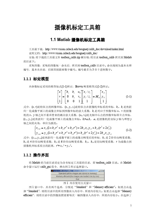
Matlab标定工具箱的使用

1
内存使用方式后，弹出标定工具箱操作面板。图 2 是选择“Standard”后弹出的标定工具箱操作面板。
图 2 标定工具箱操作面板图 2 所示的标定工具箱操作面板具有 16 个操作命令键，其功能如下： (1) “Image names”键：指定图像的基本名(Basename)和图像格式，并将相应的图像读入内存。 (2) “Read names”键：将指定基本名和格式的图像读入内存。 (3) “Extract grid corners”键：提取网格角点。 (4) “Calibration”键：内参数标定。 (5) “Show Extrinsic”键：以图形方式显示摄像机与标定靶标之间的关系。 (6) “Project on images”键：按照摄像机的内参数以及摄像机的外参数(即靶标坐标系相对于摄像机坐标系的变换关系)，根据网格点的笛卡尔空间坐标，将网格角点反投影到图像空间。 (7) “Analyse error”键：图像空间的误差分析 (8) “Recomp. corners”键：重新提取网格角点。 (9) “Add/Suppress images”键：增加/删除图像。 (10) “Save”键：保存标定结果。将内参数标定结果以及摄像机与靶标之间的外参数保存为 m 文件 Calib_results.m，存放于 toolbox_calib 目录中。 (11) “ Load ”键：读入标定结果。从存放于 toolbox_calib 目录中的标定结果文件 Calib_results.mat 读入。 (12) “Exit”键：退出标定。 (13) “Comp. Extrinsic”键：计算外参数。 (14) “Undistort image”键：生成消除畸变后的图像并保存。 (15) “Export calib data”键：输出标定数据。分别以靶标坐标系中的平面坐标和图像中的图像坐标，将每一幅靶标图像的角点保存为两个 tex 文件。 (16) “Show calib results”键：显示标定结果。

NXP SCM-i.MX 6 Series Yocto Linux 用户指南说明书

© 2017 NXP B.V.SCM-i.MX 6 Series Yocto Linux User'sGuide1. IntroductionThe NXP SCM Linux BSP (Board Support Package) leverages the existing i.MX 6 Linux BSP release L4.1.15-2.0.0. The i.MX Linux BSP is a collection of binary files, source code, and support files that can be used to create a U-Boot bootloader, a Linux kernel image, and a root file system. The Yocto Project is the framework of choice to build the images described in this document, although other methods can be also used.The purpose of this document is to explain how to build an image and install the Linux BSP using the Yocto Project build environment on the SCM-i.MX 6Dual/Quad Quick Start (QWKS) board and the SCM-i.MX 6SoloX Evaluation Board (EVB). This release supports these SCM-i.MX 6 Series boards:• Quick Start Board for SCM-i.MX 6Dual/6Quad (QWKS-SCMIMX6DQ)• Evaluation Board for SCM-i.MX 6SoloX (EVB-SCMIMX6SX)NXP Semiconductors Document Number: SCMIMX6LRNUGUser's GuideRev. L4.1.15-2.0.0-ga , 04/2017Contents1. Introduction........................................................................ 1 1.1. Supporting documents ............................................ 22. Enabling Linux OS for SCM-i.MX 6Dual/6Quad/SoloX .. 2 2.1. Host setup ............................................................... 2 2.2. Host packages ......................................................... 23.Building Linux OS for SCM i.MX platforms .................... 3 3.1. Setting up the Repo utility ...................................... 3 3.2. Installing Yocto Project layers ................................ 3 3.3. Building the Yocto image ....................................... 4 3.4. Choosing a graphical back end ............................... 4 4. Deploying the image .......................................................... 5 4.1. Flashing the SD card image .................................... 5 4.2. MFGTool (Manufacturing Tool) ............................ 6 5. Specifying displays ............................................................ 6 6. Reset and boot switch configuration .................................. 7 6.1. Boot switch settings for QWKS SCM-i.MX 6D/Q . 7 6.2. Boot switch settings for EVB SCM-i.MX 6SoloX . 8 7. SCM uboot and kernel repos .............................................. 8 8. References.......................................................................... 8 9.Revision history (9)Enabling Linux OS for SCM-i.MX 6Dual/6Quad/SoloX1.1. Supporting documentsThese documents provide additional information and can be found at the NXP webpage (L4.1.15-2.0.0_LINUX_DOCS):•i.MX Linux® Release Notes—Provides the release information.•i.MX Linux® User's Guide—Contains the information on installing the U-Boot and Linux OS and using the i.MX-specific features.•i.MX Yocto Project User's Guide—Contains the instructions for setting up and building the Linux OS in the Yocto Project.•i.MX Linux®Reference Manual—Contains the information about the Linux drivers for i.MX.•i.MX BSP Porting Guide—Contains the instructions to port the BSP to a new board.These quick start guides contain basic information about the board and its setup:•QWKS board for SCM-i.MX 6D/Q Quick Start Guide•Evaluation board for SCM-i.MX 6SoloX Quick Start Guide2. Enabling Linux OS for SCM-i.MX 6Dual/6Quad/SoloXThis section describes how to obtain the SCM-related build environment for Yocto. This assumes that you are familiar with the standard i.MX Yocto Linux OS BSP environment and build process. If you are not familiar with this process, see the NXP Yocto Project User’s Guide (available at L4.1.15-2.0.0_LINUX_DOCS).2.1. Host setupTo get the Yocto Project expected behavior on a Linux OS host machine, install the packages and utilities described below. The hard disk space required on the host machine is an important consideration. For example, when building on a machine running Ubuntu, the minimum hard disk space required is about 50 GB for the X11 backend. It is recommended that at least 120 GB is provided, which is enough to compile any backend.The minimum recommended Ubuntu version is 14.04, but the builds for dizzy work on 12.04 (or later). Earlier versions may cause the Yocto Project build setup to fail, because it requires python versions only available on Ubuntu 12.04 (or later). See the Yocto Project reference manual for more information.2.2. Host packagesThe Yocto Project build requires that the packages documented under the Yocto Project are installed for the build. Visit the Yocto Project Quick Start at /docs/current/yocto-project-qs/yocto-project-qs.html and check for the packages that must be installed on your build machine.The essential Yocto Project host packages are:$ sudo apt-get install gawk wget git-core diffstat unzip texinfo gcc-multilib build-essential chrpath socat libsdl1.2-devThe i.MX layers’ host packages for the Ubuntu 12.04 (or 14.04) host setup are:$ sudo apt-get install libsdl1.2-dev xterm sed cvs subversion coreutils texi2html docbook-utils python-pysqlite2 help2man make gcc g++ desktop-file-utils libgl1-mesa-dev libglu1-mesa-dev mercurial autoconf automake groff curl lzop asciidocThe i.MX layers’ host packages for the Ubuntu 12.04 host setup are:$ sudo apt-get install uboot-mkimageThe i.MX layers’ host packages for the Ubuntu 14.04 host s etup are:$ sudo apt-get install u-boot-toolsThe configuration tool uses the default version of grep that is on your build machine. If there is a different version of grep in your path, it may cause the builds to fail. One workaround is to rename the special versi on to something not containing “grep”.3. Building Linux OS for SCM i.MX platforms3.1. Setting up the Repo utilityRepo is a tool built on top of GIT, which makes it easier to manage projects that contain multiple repositories that do not have to be on the same server. Repo complements the layered nature of the Yocto Project very well, making it easier for customers to add their own layers to the BSP.To install the Repo utility, perform these steps:1.Create a bin folder in the home directory.$ mkdir ~/bin (this step may not be needed if the bin folder already exists)$ curl /git-repo-downloads/repo > ~/bin/repo$ chmod a+x ~/bin/repo2.Add this line to the .bashrc file to ensure that the ~/bin folder is in your PATH variable:$ export PATH=~/bin:$PATH3.2. Installing Yocto Project layersAll the SCM-related changes are collected in the new meta-nxp-imx-scm layer, which is obtained through the Repo sync pointing to the corresponding scm-imx branch.Make sure that GIT is set up properly with these commands:$ git config --global "Your Name"$ git config --global user.email "Your Email"$ git config --listThe NXP Yocto Project BSP Release directory contains the sources directory, which contains the recipes used to build, one (or more) build directories, and a set of scripts used to set up the environment. The recipes used to build the project come from both the community and NXP. The Yocto Project layers are downloaded to the sources directory. This sets up the recipes that are used to build the project. The following code snippets show how to set up the SCM L4.1.15-2.0.0_ga Yocto environment for the SCM-i.MX 6 QWKS board and the evaluation board. In this example, a directory called fsl-arm-yocto-bsp is created for the project. Any name can be used instead of this.Building Linux OS for SCM i.MX platforms3.2.1. SCM-i.MX 6D/Q quick start board$ mkdir fsl-arm-yocto-bsp$ cd fsl-arm-yocto-bsp$ repo init -u git:///imx/fsl-arm-yocto-bsp.git -b imx-4.1-krogoth -m scm-imx-4.1.15-2.0.0.xml$ repo sync3.2.2. SCM-i.MX 6SoloX evaluation board$ mkdir my-evb_6sxscm-yocto-bsp$ cd my-evb_6sxscm-yocto-bsp$ repo init -u git:///imx/fsl-arm-yocto-bsp.git -b imx-4.1-krogoth -m scm-imx-4.1.15-2.0.0.xml$ repo sync3.3. Building the Yocto imageNote that the quick start board for SCM-i.MX 6D/Q and the evaluation board for SCM-i.MX 6SoloX are commercially available with a 1 GB LPDDR2 PoP memory configuration.This release supports the imx6dqscm-1gb-qwks, imx6dqscm-1gb-qwks-rev3, and imx6sxscm-1gb-evb. Set the machine configuration in MACHINE= in the following section.3.3.1. Choosing a machineChoose the machine configuration that matches your reference board.•imx6dqscm-1gb-qwks (QWKS board for SCM-i.MX 6DQ with 1 GB LPDDR2 PoP)•imx6dqscm-1gb-qwks-rev3 (QWKS board Rev C for SCM-i.MX 6DQ with 1GB LPDDR2 PoP) •imx6sxscm-1gb-evb (EVB for SCM-i.MX 6SX with 1 GB LPDDR2 PoP)3.4. Choosing a graphical back endBefore the setup, choose a graphical back end. The default is X11.Choose one of these graphical back ends:•X11•Wayland: using the Weston compositor•XWayland•FrameBufferSpecify the machine configuration for each graphical back end.The following are examples of building the Yocto image for each back end using the QWKS board for SCM-i.MX 6D/Q and the evaluation board for SCM-i.MX 6SoloX. Do not forget to replace the machine configuration with what matches your reference board.3.4.1. X11 image on QWKS board Rev C for SCM-i.MX 6D/Q$ DISTRO=fsl-imx-x11 imx6dqscm-1gb-qwks-rev3 source fsl-setup-release.sh -b build-x11$ bitbake fsl-image-gui3.4.2. FrameBuffer image on evaluation board for SCM-i.MX 6SX$ DISTRO=fsl-imx-fb MACHINE=imx6sxscm-1gb-evb source fsl-setup-release.sh –b build-fb-evb_6sxscm$ bitbake fsl-image-qt53.4.3. XWayland image on QWKS board for SCM-i.MX 6D/Q$ DISTRO=fsl-imx-xwayland MACHINE=imx6dqscm-1gb-qwks source fsl-setup-release.sh –b build-xwayland$ bitbake fsl-image-gui3.4.4. Wayland image on QWKS board for SCM-i.MX 6D/Q$ DISTRO=fsl-imx-wayland MACHINE=imx6dqscm-1gb-qwks source fsl-setup-release.sh -b build-wayland$ bitbake fsl-image-qt5The fsl-setup-release script installs the meta-fsl-bsp-release layer and configures theDISTRO_FEATURES required to choose the graphical back end. The –b parameter specifies the build directory target. In this build directory, the conf directory that contains the local.conf file is created from the setup where the MACHINE and DISTRO_FEATURES are set. The meta-fslbsp-release layer is added into the bblayer.conf file in the conf directory under the build directory specified by the –e parameter.4. Deploying the imageAfter the build is complete, the created image resides in the <build directory>/tmp/deploy/images directory. The image is (for the most part) specific to the machine set in the environment setup. Each image build creates the U-Boot, kernel, and image type based on the IMAGE_FSTYPES defined in the machine configuration file. Most machine configurations provide the SD card image (.sdcard), ext4, and tar.bz2. The ext4 is the root file system only. The .sdcard image contains the U-Boot, kernel, and rootfs, completely set up for use on an SD card.4.1. Flashing the SD card imageThe SD card image provides the full system to boot with the U-Boot and kernel. To flash the SD card image, run this command:$ sudo dd if=<image name>.sdcard of=/dev/sd<partition> bs=1M && syncFor more information about flashing, see “P reparing an SD/MMC Card to Boot” in the i.MX Linux User's Guide (document IMXLUG).Specifying displays4.2. MFGTool (Manufacturing Tool)MFGTool is one of the ways to place the image on a device. To download the manufacturing tool for the SCM-i.MX 6D/Q and for details on how to use it, download the SCM-i.MX 6 Manufacturing Toolkit for Linux 4.1.15-2.0.0 under the "Downloads" tab from /qwks-scm-imx6dq. Similarly, download the manufacturing tool for the SCM-i.MX 6SoloX evaluation board under the "Downloads" tab from /evb-scm-imx6sx.5. Specifying displaysSpecify the display information on the Linux OS boot command line. It is not dependent on the source of the Linux OS image. If nothing is specified for the display, the settings in the device tree are used. Find the specific parameters in the i.MX 6 Release Notes L4.1.15-2.0.0 (available at L4.1.15-2.0.0_LINUX_DOCS). The examples are shown in the following subsections. Interrupt the auto-boot and enter the following commands.5.1.1. Display options for QWKS board for SCM-i.MX 6D/QHDMI displayU-Boot > setenv mmcargs 'setenv bootargs console=${console},${baudrate} ${smp}root=${mmcroot} video=mxcfb0:dev=hdmi,1920x1080M@60,if=RGB24'U-Boot > run bootcmd5.1.2. Display options for EVB for SCM-i.MX 6SXNote that the SCM-i.MX 6SX EVB supports HDMI with a HDMI accessory card (MCIMXHDMICARD) that plugs into the LCD connector on the EVB.Accessory boards:•The LVDS connector pairs with the NXP MCIMX-LVDS1 LCD display board.•The LCD expansion connector (parallel, 24-bit) pairs with the NXP MCIMXHDMICARD adapter board.LVDS displayU-Boot > setenv mmcargs 'setenv bootargs console=${console},${baudrate} ${smp}root=${mmcroot} ${dmfc} video=mxcfb0:dev=ldb,1024x768M@60,if=RGB666 ldb=sep0'U-Boot > run bootcmdHDMI display (dual display for the HDMI as primary and the LVDS as secondary)U-Boot > setenv mmcargs 'setenv bootargs console=${console},${baudrate} ${smp}root=${mmcroot} video=mxcfb0:dev=hdmi,1920x1080M@60,if=RGB24video=mxcfb1:dev=ldb,LDBXGA,if=RGB666'U-Boot > run bootcmdLCD displayu-boot > setenv mmcargs 'setenv bootargs ${bootargs}root=${mmcroot} rootwait rw video=mxcfb0:dev=lcd,if=RGB565'u-boot> run bootcmd6. Reset and boot switch configuration6.1. Boot switch settings for QWKS SCM-i.MX 6D/QThere are two push-button switches on the QWKS-SCMIMX6DQ board. SW1 (SW3 for QWKS board Rev B) is the system reset that resets the PMIC. SW2 is the i.MX 6Dual/6Quad on/off button that is needed for Android.There are three boot options. The board can boot either from the internal SPI-NOR flash inside the SCM-i.MX6Dual/6Quad or from either of the two SD card slots. The following table shows the switch settings for the boot options.Table 1.Boot configuration switch settingsBoot from top SD slot (SD3)Boot from bottom SD slot (SD2)Boot from internal SPI NORDefault1.References6.2. Boot switch settings for EVB SCM-i.MX 6SoloXThis table shows the jumper configuration to boot the evaluation board from the SD card slot SD3.7. SCM uboot and kernel repositoriesThe kernel and uboot patches for both SCM-i.MX 6 QWKS board and evaluation board are integrated in specific git repositories. Below are the git repos for SCM-i.MX 6 uboot and kernel:uBoot repo: /git/cgit.cgi/imx/uboot-imx.gitSCM Branch: scm-imx_v2016.03_4.1.15_2.0.0_gakernel repo: /git/cgit.cgi/imx/linux-imx.gitSCM branch: scm-imx_4.1.15_2.0.0_ga8. References1.For details about setting up the Host and Yocto Project, see the NXP Yocto Project User’s Guide(document IMXLXYOCTOUG).2.For information about downloading images using U-Boot, see “Downloading images usingU-Boot” in the i.MX Linux User's Guide (document IMXLUG).3.For information about setting up the SD/MMC card, see “P reparing an SD/MMC card to boot” inthe i.MX Linux User's Guide (document IMXLUG).9. Revision historyDocument Number: SCMIMX6LRNUGRev. L4.1.15-2.0.0-ga04/2017How to Reach Us: Home Page: Web Support: /supportInformation in this document is provided solely to enable system and softwareimplementers to use NXP products. There are no express or implied copyright licenses granted hereunder to design or fabricate any integrated circuits based on the information in this document. NXP reserves the right to make changes without further notice to any products herein.NXP makes no warranty, representation, or guarantee regarding the suitability of its products for any particular purpose, nor does NXP assume any liability arising out of the application or use of any product or circuit, and specifically disclaims any and all liability, including without limitation consequentia l or incidental damages. “Typical”parameters that may be provided in NXP data sheets and/or specifications can and do vary in different applications, and actual performance may vary over time. All operating parameters, including “typicals,” must be valida ted for each customer application by customer’s technical experts. NXP does not convey any license under its patent rights nor the rights of others. NXP sells products pursuant to standard terms and conditions of sale, which can be found at the following address: /SalesTermsandConditions .NXP, the NXP logo, NXP SECURE CONNECTIONS FOR A SMARTER WORLD, Freescale, and the Freescale logo are trademarks of NXP B.V. All other product or service names are the property of their respective owners.ARM, the ARM Powered logo, and Cortex are registered trademarks of ARM Limited (or its subsidiaries) in the EU and/or elsewhere. All rights reserved. © 2017 NXP B.V.。

Matrix软件包说明书

2nd Introduction to the Matrix packageMartin Maechler and Douglas BatesR Core Development Team******************.ethz.ch,*******************September2006(typeset on August11,2023)AbstractLinear algebra is at the core of many areas of statistical computing and from its inception the S lan-guage has supported numerical linear algebra via a matrix data type and several functions and operators,such as%*%,qr,chol,and solve.However,these data types and functions do not provide direct accessto all of the facilities for eﬃcient manipulation of dense matrices,as provided by the Lapack subroutines,and they do not provide for manipulation of sparse matrices.The Matrix package provides a set of S4classes for dense and sparse matrices that extend the basic matrix data type.Methods for a wide variety of functions and operators applied to objects from theseclasses provide eﬃcient access to BLAS(Basic Linear Algebra Subroutines),Lapack(dense matrix),CHOLMOD including AMD and COLAMD and Csparse(sparse matrix)routines.One notable char-acteristic of the package is that whenever a matrix is factored,the factorization is stored as part of theoriginal matrix so that further operations on the matrix can reuse this factorization.1IntroductionThe most automatic way to use the Matrix package is via the Matrix()function which is very similar to the standard R function matrix(),>library(Matrix)>M<-Matrix(10+1:28,4,7)>M4x7Matrix of class"dgeMatrix"[,1][,2][,3][,4][,5][,6][,7][1,]11151923273135[2,]12162024283236[3,]13172125293337[4,]14182226303438>tM<-t(M)Such a matrix can be appended to(using cbind()or rbind())or indexed,>(M2<-cbind(-1,M))4x8Matrix of class"dgeMatrix"[,1][,2][,3][,4][,5][,6][,7][,8][1,]-111151923273135[2,]-112162024283236[3,]-113172125293337[4,]-1141822263034381>M[2,1][1]12>M[4,][1]14182226303438where the last two statements show customary matrix indexing,returning a simple numeric vector each1. We assign0to some columns and rows to“sparsify”it,and some NA s(typically“missing values”in data analysis)in order to demonstrate how they are dealt with;note how we can“subassign”as usual,for classical R matrices(i.e.,single entries or whole slices at once),>M2[,c(2,4:6)]<-0>M2[2,]<-0>M2<-rbind(0,M2,0)>M2[1:2,2]<-M2[3,4:5]<-NAand then coerce it to a sparse matrix,>sM<-as(M2,"sparseMatrix")>10*sM6x8sparse Matrix of class"dgCMatrix"[1,].NA......[2,]-10NA150 (310350)[3,]...NA NA...[4,]-10.170 (330370)[5,]-10.180 (340380)[6,]........>identical(sM*2,sM+sM)[1]TRUE>is(sM/10+M2%/%2,"sparseMatrix")[1]TRUEwhere the last three calls show that multiplication by a scalar keeps sparcity,as does other arithmetic, but addition to a“dense”object does not,as you might have expected after some thought about“sensible”behavior:>sM+106x8Matrix of class"dgeMatrix"[,1][,2][,3][,4][,5][,6][,7][,8][1,]10NA101010101010[2,]9NA251010104145[3,]101010NA NA101010[4,]910271010104347[5,]910281010104448[6,]10101010101010101because there’s an additional default argument to indexing,drop=TRUE.If you add“,drop=FALSE”you will get submatrices instead of simple vectors.2Operations on our classed matrices include(componentwise)arithmetic(+,−,∗,/,etc)as partly seen above,comparison(>,≤,etc),e.g.,>Mg2<-(sM>2)>Mg26x8sparse Matrix of class"lgCMatrix"[1,].N......[2,]:N|...||[3,]...N N...[4,]:.|...||[5,]:.|...||[6,]........returning a logical sparse matrix.When interested in the internal str ucture,str()comes handy,and we have been using it ourselves more regulary than print()ing(or show()ing as it happens)our matrices; alternatively,summary()gives output similar to Matlab’s printing of sparse matrices.>str(Mg2)Formal class'lgCMatrix'[package"Matrix"]with6slots..@i:int[1:16]1340113422.....@p:int[1:9]0358910101316..@Dim:int[1:2]68..@Dimnames:List of2....$:NULL....$:NULL..@x:logi[1:16]FALSE FALSE FALSE NA NA TRUE.....@factors:list()>summary(Mg2)6x8sparse Matrix of class"lgCMatrix",with16entriesi j x121FALSE241FALSE351FALSE412NA522NA623TRUE743TRUE853TRUE934NA1035NA1127TRUE1247TRUE1357TRUE1428TRUE1548TRUE1658TRUEAs you see from both of these,Mg2contains“extra zero”(here FALSE)entries;such sparse matrices may be created for diﬀerent reasons,and you can use drop0()to remove(“drop”)these extra zeros.This should never matter for functionality,and does not even show diﬀerently for logical sparse matrices,but the internal structure is more compact:3>Mg2<-drop0(Mg2)>str(Mg2@x)#length 13,was 16logi [1:13]NA NA TRUE TRUE TRUE NA ...For large sparse matrices,visualization (of the sparsity pattern)is important,and we provide image()methods for that,e.g.,>data(CAex,package ="Matrix")>print(image(CAex,main ="image(CAex)"))#print(.)needed for Sweaveimage(CAex)Dimensions: 72 x 72Column R o w204060204060−0.4−0.20.00.20.40.60.81.0Further,i.e.,in addition to the above implicitly mentioned "Ops"operators (+,*,...,<=,>,...,&which all work with our matrices,notably in conjunction with scalars and traditional matrices),the "Math"-operations (such as exp(),sin()or gamma())and "Math2"(round()etc)and the "Summary"group of functions,min(),range(),sum(),all work on our matrices as they should.Note that all these are implemented via so called group methods ,see e.g.,?Arith in R .The intention is that sparse matrices remain sparse whenever sensible,given the matrix classes and operators involved,but not content speciﬁcally. E.g.,<sparse>+<dense>gives <dense>even for the rare cases where it would be advantageous to get a <sparse>result.These classed matrices can be “indexed”(more technically “subset”)as traditional S language (and hence R )matrices,as partly seen above.This also includes the idiom M [M op num ]which returns simple vectors,>sM[sM >2][1]NA NA 151718NA NA 313334353738>sml <-sM[sM <=2]>sml [1]0-10-1-10NA NA 000000000NA[24]NA 0000000and “subassign”ment similarly works in the same generality as for traditional S language matrices.41.1Matrix package for numerical linear algebraLinear algebra is at the core of many statistical computing techniques and,from its inception,the S language has supported numerical linear algebra via a matrix data type and several functions and operators,such as %*%,qr,chol,and solve.Initially the numerical linear algebra functions in R called underlying Fortran routines from the Linpack(Dongarra et al.,1979)and Eispack(Smith et al.,1976)libraries but over the years most of these functions have been switched to use routines from the Lapack(Anderson et al.,1999) library which is the state-of-the-art implementation of numerical dense linear algebra.Furthermore,R can be conﬁgured to use accelerated BLAS(Basic Linear Algebra Subroutines),such as those from the Atlas(Whaley et al.,2001)project or other ones,see the R manual“Installation and Administration”.Lapack provides routines for operating on several special forms of matrices,such as triangular matrices and symmetric matrices.Furthermore,matrix decompositions like the QR decompositions produce multiple output components that should be regarded as parts of a single object.There is some support in R for operations on special forms of matrices(e.g.the backsolve,forwardsolve and chol2inv functions)and for special structures(e.g.a QR structure is implicitly deﬁned as a list by the qr,qr.qy,qr.qty,and related functions)but it is not as fully developed as it could be.Also there is no direct support for sparse matrices in R although Koenker and Ng(2003)have developed the SparseM package for sparse matrices based on SparseKit.The Matrix package provides S4classes and methods for dense and sparse matrices.The methods for dense matrices use Lapack and BLAS.The sparse matrix methods use CHOLMOD(Davis,2005a), CSparse(Davis,2005b)and other parts(AMD,COLAMD)of Tim Davis’“SuiteSparse”collection of sparse matrix libraries,many of which also use BLAS.Todo:triu(),tril(),diag(),...and as(.,.),but of course only when they’ve seen a few diﬀerent ones.Todo:matrix operators include%*%,crossprod(),tcrossprod(),solve()Todo:expm()is the matrix exponential......Todo:symmpart()and skewpart()compute the symmetric part,(x+t(x))/2and the skew-symmetric part,(x-t(x))/2of a matrix x.Todo:factorizations include Cholesky()(or chol()),lu(),qr()(not yet for dense)Todo:Although generally the result of an operation on dense matrices is a dgeMatrix,certain operations return matrices of special types.Todo: E.g.show the distinction between t(mm)%*%mm and crossprod(mm).2Matrix ClassesThe Matrix package provides classes for real(stored as double precision),logical and so-called“pattern”(binary)dense and sparse matrices.There are provisions to also provide integer and complex(stored as double precision complex)matrices.Note that in R,logical means entries TRUE,FALSE,or NA.To store just the non-zero pattern for typical sparse matrix algorithms,the pattern matrices are binary,i.e.,conceptually just TRUE or FALSE.In Matrix, the pattern matrices all have class names starting with"n"(patter n).2.1Classes for dense matricesFor the sake of brevity,we restrict ourselves to the real(d ouble)classes,but they are paralleled by l ogical and patter n matrices for all but the positive deﬁnite ones.dgeMatrix Real matrices in general storage modedsyMatrix Symmetric real matrices in non-packed storagedspMatrix Symmetric real matrices in packed storage(one triangle only)5dtrMatrix Triangular real matrices in non-packed storagedtpMatrix Triangular real matrices in packed storage(triangle only)dpoMatrix Positive semi-deﬁnite symmetric real matrices in non-packed storagedppMatrix ditto in packed storageMethods for these classes include coercion between these classes,when appropriate,and coercion to the matrix class;methods for matrix multiplication(%*%);cross products(crossprod),matrix norm(norm); reciprocal condition number(rcond);LU factorization(lu)or,for the poMatrix class,the Cholesky decom-position(chol);and solutions of linear systems of equations(solve).Whenever a factorization or a decomposition is calculated it is preserved as a(list)element in the factors slot of the original object.In this way a sequence of operations,such as determining the condition number of a matrix then solving a linear system based on the matrix,do not require multiple factorizations of the same matrix nor do they require the user to store the intermediate results.2.2Classes for sparse matricesUsed for large matrices in which most of the elements are known to be zero(or FALSE for logical and binary (“pattern”)matrices).Sparse matrices are automatically built from Matrix()whenever the majority of entries is zero(or FALSE respectively).Alternatively,sparseMatrix()builds sparse matrices from their non-zero entries and is typically recommended to construct large sparse matrices,rather than direct calls of new().Todo: E.g.model matrices created from factors with a large number of levelsTodo:or from spline basis functions(e.g.COBS,package cobs),etc.Todo:Other uses include representations of graphs.indeed;good you mentioned it!particularly since we still have the interface to the graph package.I think I’d like to draw one graph in that article—maybe the undirected graph corresponding to a crossprod()result of dimension ca.502Todo:Specialized algorithms can give substantial savings in amount of storage used and execution time of operations.Todo:Our implementation is based on the CHOLMOD and CSparse libraries by Tim Davis.2.3Representations of sparse matrices2.3.1Triplet representation(TsparseMatrix)Conceptually,the simplest representation of a sparse matrix is as a triplet of an integer vector i giving the row numbers,an integer vector j giving the column numbers,and a numeric vector x giving the non-zero values in the matrix.2In Matrix,the TsparseMatrix class is the virtual class of all sparse matrices in triplet representation.Its main use is for easy input or transfer to other classes.As for the dense matrices,the class of the x slot may vary,and the subclasses may be triangular, symmetric or unspeciﬁed(“general”),such that the TsparseMatrix class has several3‘actual”subclasses,the most typical(numeric,general)is dgTMatrix:>getClass("TsparseMatrix")#(i,j,Dim,Dimnames)slots are common to allVirtual Class"TsparseMatrix"[package"Matrix"]Slots:2For eﬃciency reasons,we use“zero-based”indexing in the Matrix package,i.e.,the row indices i are in0:(nrow(.)-1)and the column indices j accordingly.3the3×3actual subclasses of TsparseMatrix are the three structural kinds,namely t riangular,s ymmetric and g eneral, times three entry classes,d ouble,l ogical,and patter n.6Name:i j Dim DimnamesClass:integer integer integer listExtends:Class"sparseMatrix",directlyClass"Matrix",by class"sparseMatrix",distance2Class"mMatrix",by class"Matrix",distance3Class"replValueSp",by class"Matrix",distance3Known Subclasses:"ngTMatrix","ntTMatrix","nsTMatrix","lgTMatrix","ltTMatrix", "lsTMatrix","dgTMatrix","dtTMatrix","dsTMatrix">getClass("dgTMatrix")Class"dgTMatrix"[package"Matrix"]Slots:Name:i j Dim Dimnames x factorsClass:integer integer integer list numeric listExtends:Class"TsparseMatrix",directlyClass"dsparseMatrix",directlyClass"generalMatrix",directlyClass"dMatrix",by class"dsparseMatrix",distance2Class"sparseMatrix",by class"dsparseMatrix",distance2Class"compMatrix",by class"generalMatrix",distance2Class"Matrix",by class"TsparseMatrix",distance3Class"xMatrix",by class"dMatrix",distance3Class"mMatrix",by class"Matrix",distance4Class"replValueSp",by class"Matrix",distance4Note that the order of the entries in the(i,j,x)vectors does not matter;consequently,such matrices are not unique in their representation.42.3.2Compressed representations:CsparseMatrix and RsparseMatrixFor most sparse operations we use the compressed column-oriented representation(virtual class CsparseMatrix) (also known as“csc”,“compressed sparse column”).Here,instead of storing all column indices j,only the start index of every column is stored.Analogously,there is also a compressed sparse row(csr)representation,which e.g.is used in in the SparseM package,and we provide the RsparseMatrix for compatibility and completeness purposes,in ad-dition to basic coercion((as(.,<cl>)between the classes.These compressed representations remove the redundant row(column)indices and provide faster access to a given location in the matrix because you only need to check one row(column).There are certain advantages5to csc in systems like R,Octave and Matlab where dense matrices are stored in column-major order,therefore it is used in sparse matrix libraries such as CHOLMOD or CSparse 4Furthermore,there can be repeated(i,j)entries with the customary convention that the corresponding x entries are addedto form the matrix element m ij.5routines can make use of high-level(“level-3”)BLAS in certain sparse matrix computations7of which we make use.For this reason,the CsparseMatrix class and subclasses are the principal classes for sparse matrices in the Matrix package.The Matrix package provides the following classes for sparse matrices ...FIXME many more —maybe ex plain naming scheme?...dgTMatrix general,numeric,sparse matrices in (a possibly redundant)triplet form.This can be a conve-nient form in which to construct sparse matrices.dgCMatrix general,numeric,sparse matrices in the (sorted)compressed sparse column format.dsCMatrix symmetric,real,sparse matrices in the (sorted)compressed sparse column format.Only theupper or the lower triangle is stored.Although there is provision for both forms,the lower triangle form works best with TAUCS.dtCMatrix triangular,real,sparse matrices in the (sorted)compressed sparse column format.Todo:Can also read and write the Matrix Market and read the Harwell-Boeing representations.Todo:Can convert from a dense matrix to a sparse matrix (or use the Matrix function)but going through an intermediate dense matrix may cause problems with the amount of memory required.Todo:similar range of operations as for the dense matrix classes.3More detailed examples of “Matrix”operationsHave seen drop0()above,showe a nice double example (where you see “.”and “0”).Show the use of dim<-for resizing a (sparse)matrix.Maybe mention nearPD().Todo:Solve a sparse least squares problem and demonstrate memory /speed gain Todo:mention lme4and lmer(),maybe use one example to show the matrix sizes.4Notes about S4classes and methods implementationMaybe we could give some glimpses of implementations at least on the R level ones?Todo:The class hierarchy:a non-trivial tree where only the leaves are “actual”classes.Todo:The main advantage of the multi-level hierarchy is that methods can often be deﬁned on a higher (virtual class)level which ensures consistency [and saves from “cut &paste”and forgetting things]Todo:Using Group Methods5Session Info>toLatex(sessionInfo())•R version 4.3.1Patched (2023-08-09r84931),x86_64-pc-linux-gnu•Locale:LC_CTYPE=de_CH.UTF-8,LC_NUMERIC=C ,LC_TIME=en_US.UTF-8,LC_COLLATE=C ,LC_MONETARY=en_US.UTF-8,LC_MESSAGES=de_CH.UTF-8,LC_PAPER=de_CH.UTF-8,LC_NAME=C ,LC_ADDRESS=C ,LC_TELEPHONE=C ,LC_MEASUREMENT=de_CH.UTF-8,LC_IDENTIFICATION=C •Time zone:Europe/Zurich •TZcode source:system (glibc)•Running under:Fedora Linux 36(Thirty Six)•Matrix products:default8•BLAS:/u/maechler/R/D/r-patched/F36-64-inst/lib/libRblas.so•LAPACK:/usr/lib64/liblapack.so.3.10.1•Base packages:base,datasets,grDevices,graphics,methods,stats,utils•Other packages:Matrix1.6-1•Loaded via a namespace(and not attached):compiler4.3.1,grid4.3.1,lattice0.21-8,tools4.3.1 ReferencesE.Anderson,Z.Bai,C.Bischof,S.Blackford,J.Demmel,J.Dongarra,J.Du Croz,A.Greenbaum,S.Ham-marling,A.McKenney,and PACK Users’Guide.SIAM,Philadelphia,PA,3rd edition, 1999.Tim Davis.CHOLMOD:sparse supernodal Cholesky factorization and update/downdate. http://www.cise.uﬂ.edu/research/sparse/cholmod,2005a.Tim Davis.CSparse:a concise sparse matrix package.http://www.cise.uﬂ.edu/research/sparse/CSparse, 2005b.Jack Dongarra,Cleve Moler,Bunch,and G.W.Stewart.Linpack Users’Guide.SIAM,1979.Roger Koenker and Pin Ng.SparseM:A sparse matrix package for R.J.of Statistical Software,8(6),2003.B.T.Smith,J.M.Boyle,J.J.Dongarra,B.S.Garbow,Y.Ikebe,V.C.Klema,and C.B.Moler.Matrix Eigensystem Routines.EISPACK Guide,volume6of Lecture Notes in Computer Science.Springer-Verlag, New York,1976.R.Clint Whaley,Antoine Petitet,and Jack J.Dongarra.Automated empirical optimization of software and the ATLAS project.Parallel Computing,27(1–2):3–35,2001.Also available as University of Tennessee LAPACK Working Note#147,UT-CS-00-448,2000(/lapack/lawns/lawn147.ps).9。

VIBRO_4_Acoustic_Transparency-ACTRAN隔声量分析理论

Acoustic Transparancy Computations with ACTRANACTRAN Training – VIBROCopyright Free Field TechnologiesIntroductionPre-requisites - before going through this presentation, the reader should have read and understood the following presentations:Theory ACTRAN Acoustics basic; Theory VIBRO DIRECT Simulation;These slides present the different concepts and modeling tools for computing Transmission Loss (TL) indexes in ACTRAN.2Copyright Free Field TechnologiesContentAcoustic TransparencyModeling Acoustic Transparency with ACTRANDiffuse sound fieldRayleigh surface3Copyright Free Field TechnologiesAcoustic TransparencyAcoustic transparency generally defined a group of standard tests performed to assess the ability of a component to attenuate soundThe standard tests of acoustic transparency generally involved 2 rooms acoustically connected by the system to be testedThe typical indicator used in Acoustic Transparency is the Transmission Loss index (TL)4Copyright Free Field TechnologiesWhat is the transmission loss index?Transmission loss:Symbols used in the literature: TL, STL or R expressed in dB Intrinsic property of system (does not depend on the coupled rooms of the set-up)TL = 10 ⋅ log10(1 τ )[ dB ]withτ (ω ) = Wtransmitted / WincidentThe transmission loss is the logarithmic representation of the ratio of powers: what is the part of the incident power that will be transmitted through the studied structure.5Copyright Free Field TechnologiesTypical measurement set-up: associated chambersAnechoic and reverberant rooms can be associated: side by side (classic transmission loss measurements) or on top of each other (building impact noise). Most used set-up: two side-by-side reverberant rooms 6Copyright Free Field TechnologiesTypical measurement set-up: associated reverberant chambersASTM E90 STL = SPL(source room) – SPL(receiving room) +10 log S – 10 log A(receiving room surface) [dB] S = area of test specimen (common to both rooms) A = sound absorption of receiving room with test specimen in place (metric Sabins) STL = R = TL = sound transmission loss index The sound pressure level (SPL) is measured in each rooms using a rotating microphone (pressure average). The sound absorption can be derived from reverberation time measurement7Copyright Free Field TechnologiesSimplified experimental set-upsTwo small chambers test set-up8Copyright Free Field TechnologiesSimplified experimental set-upsSmall cabin test set-up9Copyright Free Field TechnologiesContentAcoustic TransparencyModeling Acoustic Transparency with ACTRANDiffuse sound fieldRayleigh surfaces10Copyright Free Field TechnologiesReal ProblemExperimental Set up to be modeled:Anechoic Receiving Room Measurement ofIncident PowerMeasurement ofRadiated PowerReverberant Room withDiffuse Sound FieldSystem to be characterizedACTRAN Modeling Strategy (1)The Diffuse Sound Field (DSF) excitation available in ACTRAN can be used to simulated the incident sound field loading the systemThe reverberant room is not modeled. The DSF boundary condition is applied on the loaded surfaceThe incident power over the surface is automatically computedThe Rayleigh Surface component or the Infinite Fluid Component can be used to model the radiation in free fieldNo or limited modeling of the receiving roomThe power radiated by the system is automatically outputThe PLTViewer viewer has a TL operator to quickly plot the TL index from the PLT file computedACTRAN offers two different ways to model free field radiation of baffled structures :A combination of a Finite Fluidand an Infinite Fluid components The definition of aRayleigh Surface componentFinite Fluid DomainInterest of Rayleigh Surface:Reduction of the meshing effortReduced number of degrees of freedomDisadvantages of Rayleigh Surface :Limited to plane or nearly plane baffled structuresLimits of the ModelingThe acoustic field of a reverberant chamber is no longer diffuse under a cut-off frequency that depends on the room size and shapeComparison between test and simulation below the cut-off frequency should be done with careThe fixation of the system is ideal in the simulation while it may not be perfect in the realityThis may explain discrepancies between the test and simulation resultsContentAcoustic TransparencyModeling Acoustic Transparency with ACTRAN Diffuse sound fieldRayleigh surfacesThe set of a Diffuse Sound Field boundary condition is done in 2 stepsDefine the parameter of DSFSpecify the surface of application through an Incident Surface post-processing componentThe Diffuse Sound Field Boundary Condition(1)TypeInput Power Spectral Density (PSD)Properties of the reverberant roomNumber of samples simulatedThe Diffuse Sound Field Boundary ConditionDiffuse field :“Sound field in which the time average of the mean-square sound pressure is everywhere the same and the flow of acoustic energy in all directions is equally probable.”(INCE)Diffuse fields are produced experimentally by activating strong acoustic sources in a reverberant chamber, the multiple reflections along the boundary wallsleading to a “diffuse” field.Association of an Incident Surface to the DSF excitationAdd a new Incident Surface post-processing component Drag’nDrop the surface mesh of applicationDrag’nDrop the Incident Surface to the DSF excitationThe Diffuse Sound Field Boundary Condition(2)The Diffuse Sound Field –Element of Theory(1)The Diffuse Sound Field is considered as a weakly stationary random processThe DSF is characterized by the cross-correlation function betweeneach pair of loaded nodes The input of a Random excitation is given in term of Power Spectral ()rk r k f ⋅⋅=sin Density (PSD)(2)The strategy to compute the response of a system under a DSF is to: Perform a Cholesky decomposition of the DSF matrixCompute the response of the system to a large number of samplesCompute the average response to the samplesOutput PSD= Σ(Output sample)²It is advise to set at least 30 samplesThe PSD response is automatically computed when a PSD_FILENAME is provided(3)For further information about the Random excitations and their full theory, please refer to the VIBRO_RANDOM_Simulation.pdfpresentationContentAcoustic TransparencyModeling Acoustic Transparency with ACTRAN Diffuse sound fieldRayleigh surfacesRayleigh Surfaces DefinitionThe acoustic field related to a baffled plane (or nearly plane) structure can be modeled using the Rayleigh boundary integral representation :∫ρω=S n 2)y (dS )y ,x (G )y (u )x (p Rigid plane Rayleigh surface Field pointsField point can be defined to retrieve de pressure in the far field Rigid plane Vibrating plateThe Rayleigh Surface Component (2)Syntax in the ACTRAN input file: Definition in ACTRAN/VIBEGIN RAYLEIGH_SURFACE surface_idMATERIAL material_idnumber of faceList of facesEND RAYLEIGH_SURFACE surface_idDomainGoing FurtherThe concepts that have been presented are put in practice in the workshop Workshop_VIBRO_4_Windshield.pdf。

1、下载文档前请自行甄别文档内容的完整性，平台不提供额外的编辑、内容补充、找答案等附加服务。
2、"仅部分预览"的文档,不可在线预览部分如存在完整性等问题,可反馈申请退款(可完整预览的文档不适用该条件!)。
3、如文档侵犯您的权益，请联系客服反馈,我们会尽快为您处理(人工客服工作时间：9:00-18:30)。

IDS InnomicGesellschaft für Computer- und Messtechnik mbHInstruction ManualVibroMatrix Instruction ManualVersion: 1.6.0.71, 02/06/2009Authors:Dipl.Ing. Thomas Olschewski, Dr.rer.nat. Thomas DamkerIDS Innomic Gesellschaft für Computer- und Messtechnik mbHZum Buchhorst 2529410 SalzwedelGermany© 2003 – 2009 All rights reserved. Reproduction (also in extracts) only with permission of IDS Innomic GmbH.VibroMatrix®InnoBeamer®InnoMaster®InnoStreamMachine®InnoMeter®InnoLogger®InnoPlotter®InnoAnalyzer®InnoScope®InnoBalancer®are registered trademarks of IDS Innomic GmbHWindows®is registered trademark of Microsoft CorporationDespite accurate work we cannot exclude errors in this manual. We hereby disclaim all warranties and conditions related to this informa-tion regarding fitness for a particular purpose and non-infringement. In no event shall IDS Innomic GmbH and/or its respective suppliers be liable for any special, indirect or consequential damages or any damages whatsoever resulting from loss of use, data or profits, whether in an action of contract, negligence or other tortuous action arising out of or in connection with the use of information available in this manual.Contents1.Introduction (6)1.1.Overview (7)2.Quick Start (8)2.1.What you need (8)2.2.How to proceed (8)3.How to install VibroMatrix on your PC (9)3.1.Driver installation (9)3.2.VibroMatrix installation (11)4.Vibration sensors and measurement devices (14)4.1.Piezoelectric accelerometers (14)Overview (14)Sensor mounting (14)4.2.InnoBeamer® – Connecting sensor and PC (15)InnoBeamer L2 (16)Measuring ranges with selected sensors (16)5.The control center InnoMaster® RT (17)5.1.Sensor Management (18)Creating a new sensor group (18)Changing the properties of a sensor group (18)Deleting a sensor group (19)Creating a new sensor entry (19)Changing sensor properties (19)Deleting a sensor (20)Assigning a sensor to a measuring channel (20)Disconnecting a sensor from the measuring channel (20)5.2.Measuring channel management (21)Changing the properties of a measuring channel (21)Deleting a disconnected InnoBeamer device (22)Showing the properties of an InnoBeamer device (22)Showing the properties of an InnoBeamer device type (22)5.3.Instrument management (22)Starting an instrument (23)Adding an instrument (23)5.4.Event messengers (24)5.5.Central start/stop button (24)5.6.Extended InnoMaster settings (25)Display settings (25)Signal processing settings (26)Workspace settings (27)Measurement data recording settings (29)6.VibroMatrix instruments (30)6.1.Overview (30)The instruments at a glance (30)6.2.Uniform control elements (31)6.3.Controls of multichannel graphical instruments (32)6.4.Report generation (37)6.5.Configuring event messengers (39)Using a messenger (40)Releasing a messenger (40)Configuring event messengers (40)6.6.Uniform status indicators (40)6.7.Calibrator – Sensor calibration for all VibroMatrix instruments (43)Displays and controls (43)6.8.InnoMeter® – Universal vibration meter with digital display (45)Overview (45)Displays and controls (46)6.9.InnoPlotter® – Digital strip chart recorder for vibration parameters (48)Overview (48)Displays and controls (49)6.10.InnoLogger® – Logging of vibration signals and vibration parameters (52)Overview (52)Displays and controls (53)Data format (57)6.11.InnoScope® – Displaying fast vibration and shock events (60)Overview (60)Displays and controls (61)6.12.InnoAnalyzer® – Frequency and vibration analysis (68)Overview (68)Displays and controls (69)6.13.InnoAnalyzer® Speed – Measurements at run-up and coast-down (73)Displays and controls (74)6.14.InnoBalancer® – Field balancing (78)Overview (78)Displays and controls (79)6.15.InnoMeter® HVM 2631:1997 – Human whole-body vibration measurement (90)Overview (90)Preparing the measurement (91)Performing the measurement (95)Data storage (99)Evaluation with exposure segments (101)Event messengers (104)6.16.InnoMeter® HVM 5349:2001 – Human hand-arm vibration measurement (105)Overview (105)Preparing the measurement (106)Performing the measurement (108)Data storage (110)Evaluation (112)Event messengers (117)6.17.InnoMeter® HVM 6954:2001 – Vibration measurement on ships (118)Overview (118)Preparing the measurement (119)Performing the measurement (121)Data storage (123)Event messengers (125)6.18.InnoMeter® 4150-3:1999 – Vibration measurement of buildings (126)Overview (126)Preparing the measurement (127)Performing the measurement (131)Data storage (134)Graphical display (136)Event messengers (137)7.Event messengers (139)7.1.Messenger administration (139)Activating the messenger administration when required (139)List of event messengers (139)Creating a messenger (140)Deleting a messenger (140)Display modes of event messengers (140)7.2.Messenger type e-mail (140)Configuration (141)7.3.Messenger type extra display (144)Configuration (144)7.4.Messenger type radio switch (145)Overview (145)Set up (145)Driver installation (146)Checking the connection with the radio control center (146)Configuration of the event messenger (147)8.InnoMaster® Replay – Off-line analysis (148)Basic process (148)8.1.Loading a data file (149)8.2.Playing back a data file (149)More tips for replaying (151)8.3.Control panel Navigator (151)The Navigator display (151)Axes menu (153)Notes menu (153)Masks menu (154)Export menu (155)8.4.Control panel Notes and Masks (156)8.5.Differences to InnoMaster RT (157)Sensor management (157)Channel management (157)Instrument management (158)Using the software instruments (158)9.Facts about VibroMatrix worth knowing (159)9.1.Technologies (159)InnoStreamMachine® – Digital data streams as kernel of VibroMatrix (159)Synchronization of measuring channels (159)9.2.Licensing software in VibroMatrix (160)Channel concept and clone function (161)1.Introduction1.IntroductionThank you for choosing VibroMatrix. You have purchased an efficient, expandable and economical solution for vibration measurement. Whether in laboratory, permanent in-dustrial installations or field, VibroMatrix can be used for each of these applications. VibroMatrix provides a variety of vibration instruments based on your PC and broadens the potential of conventional instrumentation.▪You can operate several instruments with one common vibration sensor – without any disadvantages like by electrical connection of measuring instruments.▪Duplicate your instruments during the measurement – one becomes two, three, ...▪Enlarge the number of measurement channels by additional DAQ boxes. When con-figured conveniently, measured data is read in as synchronously as it would be if only one data acquisition device was used.▪Save the screen arrangement of instruments with individual settings in workspaces. You never built up and configured your conventional instrumentation as fast as a workspace is restored.▪In case of unattended measurements, VibroMatrix now informs you when interesting events occurred, for instance by e-mail.▪Play measurements again with recorded data and analyze the measured data more in-tensely than during live measurement. Simply put comments to the data stream during live measurement. They are indicated again when replaying and help you to relate the measurement data.This instruction manual shows you how to efficiently apply VibroMatrix in order to solve your measuring tasks. If you do not have enough time to read the entire document please proceed to the chapter 2 on page 8.If you have more time to become familiar with VibroMatrix, this manual will inform you detailed about both the complete system and the system’s components, like control center and instruments.Hint: If you read this manual electronically, you can click on the page reference, like this one for instance – page 8 – to go directly to this page.The current version of the manual can always be downloaded under .We are at your disposal for increments, complaints and wishes. We are sure you will use VibroMatrix successfully.Germany, Salzwedel, February 6, 2009VibroMatrix Development Team Introduction61.Introduction 1.1.OverviewVibroMatrix is a PC based vibration measurement system consisting of harmonizedhardware and software modules. This measurement system is a complementary solutionfor your notebook or PC and is therefore very cost-efficient. Until now, your PC hasbeen your typewriter, calendar or drawing board. With VibroMatrix, it becomes a high-quality vibration measurement system. You continue using your familiar environment.1.Piezoelectric sensors with integrated amplifier are directly connected to the PC viathe InnoBeamer USB adapter. Piezoelectric sensors with charge output are previous-ly connected with a charge converter from the ICP1x0-series and thereafter are ableto transmit their signals to the PC as well.2.One or more InnoBeamers are connected to the USB interface of the PC. The PCsupplies the InnoBeamer with energy. No external power supply is required.3.The software instruments have been tailored for various measuring applications.Still, all instruments can work on the PC-screen at the same time. You can combinethem at will. The operation is performed by mouse. The results are displayed in real-time, high resolution and color.4.If required, messages can be sent automated, for instance by e-mail to another PC.The operation of VibroMatrix is simple, because the system is based on the natural sig-nal flow: sensors → measuring channels → instruments → messengers.Quick starters go on to the next page. For those with more time: Proceed like that:Installation – Your PC/notebook becomes a measuring machine........................p.9Sensors and devices provide the measurement signals .......................................p.14Control center InnoMaster – Comfortable overview ..........................................p.17Instruments – Vibrations are visible now ............................................................p.30VibroMatrix non-stop operation – Automated event messages ..........................p.139Replay – Off-line analysis of measured data.......................................................p.1482.Quick Start2.Quick StartVibroMatrix has reduced considerably the setup time since version 1.5. Before the sys-tem is delivered a complete configuration with your purchased sensors and instruments is prepared. During installation this individually created configuration is transferred to your computer an you are immediately ready for measurement.2.1.What you need▪PC or notebook with USB interface, CD-ROM drive, operating system Windows 98, Windows ME, Windows 2000, Windows XP, Windows Vista▪VibroMatrix CD-ROM▪Piezoelectric sensor with integrated amplifier▪Sensor cable with BNC plug on the InnoBeamer side▪InnoBeamer device▪USB cable2.2.How to proceed▪Switch on your PC.▪Insert the VibroMatrix CD-ROM.▪Connect InnoBeamer to your PC via USB cable.▪When Windows asks for driver installation, direct the assistant to your CD-ROM and install the driver (page 9).▪If you have more than one InnoBeamer, repeat the last step for the other InnoBeamers until all of them are connected to your PC.▪Start VibroMatrix_Setup.exe in the root directory of the CD-ROM and install the software (page 11).▪This will transfer the prepared configuration too. When you finish the installation, VibroMatrix will start with one of the pre-configured work spaces.▪Connect the sensor to the InnoBeamer, switch on the instrument, the measurement is running.How to proceed83.How to install VibroMatrix on your PC3.How to install VibroMatrix on your PCThe installation of the VibroMatrix software is executed in two steps. The driver for the InnoBeamer must be installed first. Then the VibroMatrix software itself is installed.3.1.Driver installationA driver is a small piece of software controlling the InnoBeamer hardware under Win-dows. The InnoBeamer driver is a so-called WDM driver supporting Windows 98 (first and second edition), Windows ME, Windows 2000, Windows XP and Windows Vista. For installation from Windows 2000 Professional on make sure that you have permis-sion to install drivers.When you connect the InnoBeamer to your PC for the first time, the operating system recognizes the hardware and asks you for an appropriate device driver. The drivers are located in the root directory of your VibroMatrix CD-ROM.The dialog boxes after the fist connection with the InnoBeamer vary, depending on the Windows version you are using. The following dialog, for example, applies for Win-dows XP.The hardware wizard opens, an-nouncing the installation of thedriver.Insert your VibroMatrix-CD now.Select Install the software auto-matically and click on Next >.Windows automatically searchesthe CD-Rom drive, finds the driverand installs it.3.How to install VibroMatrix on your PC A final message about the success-ful installation appears in the end.Click on Finish.It is a characteristic of some Windows versions to ask for the driver again when you connect the InnoBeamer with an USB interface it has not been connected to previously. That is why we recommend to successively connect the InnoBeamer to all USB interfaces of the PC/notebook and – if Windows asks for it – install the driver for each of them. This way, you avoid later Windows callbacks when you actu-ally just want to work with VibroMatrix.Driver installation 103.How to install VibroMatrix on your PC3.2.VibroMatrix installationBefore installation, please uninstall old versions of VibroMatrix first.The installation program VibroMatrix_Setup.exe is located in the root directory ofyour VibroMatrix CD-ROM.tains all language versions ofVibroMatrix.Please choosethe desired language first.to the installation.Click on Next >.ment informs you about theterms of use for the VibroMa-trix software.If you agree, choose the up-per option to accept the li-cense agreement and click onNext >.3.How to install VibroMatrix on your PCNow you define which direc-tory the software will be in-stalled in. A default directory has already been preset.Click on Next >.Even if the directory is al-ready present due to a former installation, you can install VibroMatrix there.Click on Yes.A summary for the upcoming installation is displayed now. Click on Install .Now the installation is carried out according to your instruc-tions.A final dialog appears in the end.If required, you can start the training program for Vibro-Matrix now. For this pro-gram, you do not need any measurement hardware.A separate training manual with many practical exercises inducts you into vibration measurement.Click on Finish .VibroMatrix installation123.How to install VibroMatrix on your PCto optionally save the signals in Innomic Data Stream format. InnoMaster Replay The control center for the replay of data saved in InnomicData Stream format.InnoMaster RT Trainer All instruments can be used without measurement hardware,thus allowing to become acquainted with their functionality.A short training program gives an introduction to vibrationmeasurement.Uninstall VibroMatrix Uninstalls the program. Measured data will not be deleted.4.Vibration sensors and measurement devices4.Vibration sensors and measurement devices4.1.Piezoelectric accelerometers OverviewPiezoelectric accelerometers with integrated amplifier are most suitable for vibration measurement. They are available from several producers for different applications. The following sensors are an example for our offer:▪General purpose accelerometers▪High sensitivity accelerometers, for instance for building vibration measurement ▪Miniature accelerometers, for instance for small objects ▪Triaxial accelerometers, for measurement in three axes ▪Industrial accelerometers▪Special sensors, for instance seat accelerometer for human vibration measurementAccelerometers with charge output can be refitted with an external remote charge con-verter.Sensor mountingBefore making measurements, suitable measuring points need to be found. On rotating machines, vibration forces are normally transmitted into the machine frame via bearings and their housings. Therefore, bearing housings or points close to bearings are recom-mended as measuring points. Less suitable are light or mechanically flexible machine parts.An even, smoothsurface at the mounting point isindispensable forprecise vibrationtransmission from the machine to theaccelerometer. Measuring pointsthat are uneven, scratched or insuf-ficiently sized may cause considerableerrors, particularly at frequencies above 1 kHz. For best transmitting conditions, we rec-ommend a stainless steel disk with vertical mounting thread which can be glued or welded onto the machine. The diameter should be at least as big as the diameter of the accelerometer.The transducer is usually mounted by stud bolts. A thin layer of grease (e.g. silicon grease) will improve the quality of the couple connection. For measurements up to 1 kHz, mounting via clamping magnet is suitable as well.Piezoelectric accelerometers144.Vibration sensors and measurement devices4.2.InnoBeamer® – Connecting sensor and PCThere is no direct connection for piezoelectric sensors on the PC. That’s why the USBadapter InnoBeamer is interposed. It digitizes the transducer signals and provides USBcompatible data for the software instruments on the PC. On the input, sensors are con-nected directly and supplied. On the output, the transfer of the digitized data via USBinterface is carried out.A safe link mode is used, which transfers all data without dropouts. Scanner, printer orother instruments can be used in parallel on the USB input of the PC.InnoBeamers receive their power supply from the USB interface of the PC. No externalpower supply is necessary. The complete measuring chain is supplied by PC, which al-lows an easy use of VibroMatrix on notebooks far away from any power outlet.4.Vibration sensors and measurement devices InnoBeamer L2Measuring ranges with selected sensorsDAQ products are often advertised by unpractical electrical properties. What counts, are maximum values and resolution of vibration quantities. The following table shows which values a VibroMatrix system provides with different sensors:InnoBeamer® – Connecting sensor and PC16Sensor: KS74BFrequency range [Hz]Acceleration [m/s²]Velocity [mm/s]min maxmin max min max min max 0,3 2000 0,00812000,3-100-1 1,1 0,000512000,04191000 630.000.000 10 11 0,000812000,00619100 0,1300.000 100 110 0,000612000,00051910 0,0008 3.000 1000 11000,001612000,0001191 0,0000230Sensor: KS80CFrequency range [Hz]Acceleration [m/s²]Velocity [mm/s]min maxmin max min max min max 0,3 2000 0,0046000,2-50-1 1,1 0,00036000,0295000 315.000.000 10 11 0,00046000,0039500 0,1150.000 100 110 0,00036000,0003950 0,0004 1.500 1000 11000,00086000,0001950,0000115Sensor: KS48BFrequency range [Hz]Acceleration [m/s²]Velocity [mm/s]min maxmin max min max min max 0,3 2000 0,0004600,08-30-1 1,1 0,00003600,00210000 0,3 1.600.000 10 11 0,00004600,00031000 0,0116.000 100 110 0,00003600,00003100 0,00004160 1000 11000,00008600,00001100,0000011,6Sensor: KB12VBFrequency range [Hz]Acceleration [m/s²]Velocity [mm/s]min maxmin max min max min max 0,3 260 0,0000260,002-0,6-1 1,1 0,00000360,00021000 0,03160.000 10 11 0,00000460,00003100 0,001 1.600 100 1100,00000360,000003100,00000416Displacement [µm]Displacement [µm]Displacement [µm]Displacement [µm]Connector and indicator for USB connectorConnector and indicator for piezoelectric sensor 25.The control center InnoMaster® RT 5.The control center InnoMaster® RTVibroMatrix is a modular system. Sensors, measuring channels, software instrumentsand – if required – event messengers are combined to solve the vibration measurementtasks. The InnoMaster RT organizes the communication between these modules.After having started VibroMatrix, this control center appears at the lower edge of yourscreen. By means of 4 buttons, all elements of the measuring chain are available.By clicking on Settings >>, further global functions are available.In both modes the CPU load of the PC is displayed. It shows how much CPU capacityis occupied by the digital signal processing of VibroMatrix. If the CPU load exceeds100%, the instruments cannot work with the required speed. In this case, instrumentsshould be closed or their refresh rate reduced (page 25). However, the optimized pro-gram code of VibroMatrix - the InnoStreamMachine - will run properly even with olderPCs. Thus, vibration measurement with VibroMatrix works on PCs from 500 MHz on.The following section explains the settings of the measuring chain followed by a de-scription of the extended functions of InnoMaster (page 25).5.The control center InnoMaster® RT 5.1.Sensor ManagementA measuring chain starts with the sensors. The InnoMaster allows to acquire and archive the data of your sensors. As soon as a sensor is assigned to a measuring channel, it will make its measured data to all instruments connected to this channel. The data is: sensor name, serial number and calibration to mV.A click on the Sensor button in the InnoMaster opens the sensor control window. A clear arrangement of the sensors data can be obtained by sensor groups.On the left side of the sensor name, there is an activityindicator. It can show 3 states:▪Red The sensor is not in use.▪Yellow: The sensor is assigned to a measuring channel but this channel is not active. ▪Green:The sensor is assigned to a measuring channel and it is involved in a measure-ment.By means of the 3 buttons in the bottom line, the dis-played sensors can be filtered. For instance, only ac-tive sensors can be displayed.By a right click in the environment of the sensor list, a context-sensitive menu opens. Its functions are ex-plained in the following section.Creating a new sensor group➔Click right in an empty space of the sensor list. A new menu named New group will open.➔Click left on this entry. A new sensor group with a default name is generated. You can change this name as described in the next section.Up to 100 sensor groups can be created.Changing the properties of a sensor group➔A property window appears automatically after a sensor group has been created. Oth-erwise, double-click left on a sensor group to open the property window.➔Enter a name for the sensor group and, if desired, a description text.If an already existing name is entered, a message will appear asking for a differentname.Sensor Management185.The control center InnoMaster® RTDeleting a sensor groupopens.➔Select Delete group and click left on it.➔A confirmation message appears. The deletion canbe confirmed or canceled.Creating a new sensor entry➔Click right on a sensor group.A context menu➔Choose New sensor and click left on it.➔A new sensor with a default name in the previouslychosen group is generated. You can change thisname in Properties.Up to 100 sensors per group can be created.Changing sensor propertieshas been created. Otherwise, double-click left on a sen-sor to open the property window.Standard sensors are piezoelectric accelerometers. Forthese sensors all measuring units,measurands,etc.arepreset.▪Type: Select one type from the list or type it in.▪Serial number: In order to distinguish the sensors, en-ter the serial number here.▪Sensitivity: The sensitivity from the data sheet of thesensor can be added here. Another method is to cali-brate the sensor with the VibroMatrix instrument Cali-brator (page 43). The calibration date (field Last cali-bration) is also updated, when the sensitivity value isconfirmed (i.e. when the enter button is pressed withinthe field Sensitivity). A regular calibration is recommended, though (12 months forintensively used equipment, 24 months otherwise).▪Calibration interval: Define the calibration interval for the sensor here. InnoMastercompares the date of the last calibration with the present one and signals the calibra-tion state automatically.- OK(green):Less than 90% of the calibration interval are expired.- Calibrate soon (yellow):More than 90% of the calibration interval are expired.- Calibrate !!!(red):The calibration interval is expired.▪Calibrate now: This button starts the VibroMatrix instrument Calibrator. Thereforethe sensor must be connected to a measuring channel (page 20).5.The control center InnoMaster® RT Deleting a sensor➔Click right on a sensor. A context menu opens.➔Select Delete sensor and click left on it.➔A confirmation message appears. The deletion can be confirmed or canceled.Assigning a sensor to a measuring channelSpecify now which sensor from the sensor list is actually connected to an InnoBeamer measuring channel. This is done with simple “drag and drop“ by your mouse.➔Open the windows Sensors and Mea-suring channels by clicking on the re-spective buttons in the InnoMaster.➔Click left on a sensor and keep the but-ton pressed.➔Drag the sensor to a measuring channel that is marked yellow or green, i.e. it must be physically connected to an In-noBeamer.➔Release the left mouse button.The sensor is connected to the measuring channel now. Thus the sensor parameters (e.g. calibrated sensitivity) are accessible for this channel. The sensor will automati-cally appear in all instruments workingwith this channel and these instruments will consider the new sensitivity instantaneous-ly.Disconnecting a sensor from the measuring channel➔Open the window for the measuring channelmanagement by clicking on the button Measuring Channels in the InnoMaster.➔Click right on a measuring channel to which a sensor was assigned previously. A context menu opens.➔Select the entry Disconnect sensor .Sensor Management205.The control center InnoMaster® RT 5.2.Measuring channel managementIn the measuring chain,sensors(page 18)are fol-To view the channel settings, open the Measuringchannels window by clicking the respective Inno-Master button: Here you find all available InnoBeam-er devices with their associated measuring channels. Ifan InnoBeamer is connected to or disconnected fromthe USB interface, the list will be updated automati-cally. The state of each measuring channel is shownby an indicator on the left. 3 states are possible:▪Red:The measuring channel belongs to an In-noBeamer device which is currently notconnected to the PC (off-line).▪Yellow: The measuring channel belongs to an InnoBeamer device which is con-nected to the PC but currently not measuring (on-line/inactive).▪Green: The measuring channel is measuring (on-line/active).On the bottom of the Measuring channels window you will find three switches whichcan be used for filtering the listed channels. For example, only active channels can belisted.Other setup features are accessible by right mouse click.Changing the properties of a measuring channel➔Double-click left on a measuring channel. A property window opens.This window shows which InnoBeamer theCoupling the input signal is processed with.You can type in an individual Name for eachmeasuring channel. It will be shown in themeasuring channel list as well as in the in-struments.The date of the Last calibration is also dis-played in the properties window. For recali-bration please contact your dealer.In the Supported instruments list you willfind all instruments which are registered forthis channel. To register one further instru-ment click on the button Add instrument orlease time for instrument. Further detailsabout Adding an instrument can be found onpage 23.。