美赛论文solution
2013美国大学生数学建模竞赛论文

summaryOur solution paper mainly deals with the following problems:·How to measure the distribution of heat across the outer edge of pans in differentshapes and maximize even distribution of heat for the pan·How to design the shape of pans in order to make the best of space in an oven·How to optimize a combination of the former two conditions.When building the mathematic models, we make some assumptions to get themto be more reasonable. One of the major assumptions is that heat is evenly distributedwithin the oven. We also introduce some new variables to help describe the problem.To solve all of the problems, we design three models. Based on the equation ofheat conduction, we simulate the distribution of heat across the outer edge with thehelp of some mathematical softwares. In addition, taking the same area of all the pansinto consideration, we analyze the rate of space utilization ratio instead of thinkingabout maximal number of pans contained in the oven. What’s more, we optimize acombination of conditions (1) and (2) to find out the best shape and build a function toshow the relation between the weightiness of both conditions and the width to lengthratio, and to illustrate how the results vary with different values of W/L and p.To test our models, we compare the results obtained by stimulation and our models, tofind that our models fit the truth well. Yet, there are still small errors. For instance, inModel One, the error is within 1.2% .In our models, we introduce the rate of satisfaction to show how even thedistribution of heat across the outer edge of a pan is clearly. And with the help ofmathematical softwares such as Matlab, we add many pictures into our models,making them more intuitively clear. But our models are not perfect and there are someshortcomings such as lacking specific analysis of the distribution of heat across theouter edge of a pan of irregular shapes. In spite of these, our models can mainlypredict the actual conditions, within reasonable range of error.For office use onlyT1 ________________T2 ________________T3 ________________T4 ________________ Team Control Number18674 Problem Chosen AFor office use only F1 ________________ F2 ________________ F3 ________________ F4 ________________2013 Mathematical Contest in Modeling (MCM) Summary Sheet(Attach a copy of this page to your solution paper.)Type a summary of your results on this page. Do not includethe name of your school, advisor, or team members on this page.The Ultimate Brownie PanAbstractWe introduce three models in the paper in order to find out the best shape for the Brownie Pan, which is beneficial to both heat conduction and space utility.The major assumption is that heat is evenly distributed within the oven. On the basis of this, we introduce three models to solve the problem.The first model deals with heat distribution. After simulative experiments and data processing, we achieve the connection between the outer shape of pans and heat distribution.The second model is mainly on the maximal number of pans contained in an oven. During the course, we use utility rate of space to describe the number. Finally, we find out the functional relation.Having combined both of the conditions, we find an equation relation. Through mathematical operation, we attain the final conclusion.IntroductionHeat usage has always been one of the most challenging issues in modern world. Not only does it has physic significance, but also it can influence each bit of our daily life. Likewise,space utilization, beyond any doubt, also contains its own strategic importance. We build three mathematic models based on underlying theory of thermal conduction and tip thermal effects.The first model describes the process and consequence of heat conduction, thus representing the temperature distribution. Given the condition that regular polygons gets overcooked at the corners, we introduced the concept of tip thermal effects into our prediction scheme. Besides, simulation technique is applied to both models for error correction to predict the final heat distribution.Assumption• Heat is distributed evenly in the oven.Obviously, an oven has its normal operating temperature, which is gradually reached actually. We neglect the distinction of temperature in the oven and the heating process, only to focus on the heat distribution of pans on the basis of their construction.Furthermore, this assumption guarantees the equivalency of the two racks.• Thermal conductivity is temperature-invariant.Thermal conductivity is a physical quantity, symbolizing the capacity of materials. Always, the thermal conductivity of metal material usually varies with different temperatures, in spite of tiny change in value. Simply, we suppose the value to be a constant.• Heat flux of boundaries keeps steady.Heat flux is among the important indexes of heat dispersion. In this transference, we give it a constant value.• Heat conduction dom inates the variation of temperature, while the effects ofheat radiation and heat convection can be neglected.Actually, the course of heat conduction, heat radiation and heat convectiondecide the variation of temperature collectively. Due to the tiny influence of other twofactors, we pay closer attention to heat conduction.• The area of ovens is a constant.I ntroduction of mathematic modelsModel 1: Heat conduction• Introduction of physical quantities:q: heat fluxλ: Thermal conductivityρ: densityc: specific heat capacityt: temperature τ: timeV q : inner heat sourceW q : thermal fluxn: the number of edges of the original polygonsM t : maximum temperaturem t : minimum temperatureΔt: change quantity of temperatureL: side length of regular polygon• Analysis:Firstly, we start with The Fourier Law:2(/)q gradt W m λ=- . (1) According to The Fourier Law, along the direction of heat conduction, positionsof a larger cross-sectional area are lower in temperature. Therefore, corners of panshave higher temperatures.Secondly, let’s analyze the course of heat conduction quantitatively.To achieve this, we need to figure out exact temperatures of each point across theouter edge of a pan and the variation law.Based on the two-dimension differential equation of heat conduction:()()V t t t c q x x y yρλλτ∂∂∂∂∂=++∂∂∂∂∂. (2) Under the assumption that heat distribution is time-independent, we get0t τ∂=∂. (3)And then the heat conduction equation (with no inner heat source)comes to:20t ∇=. (4)under the Neumann boundary condition: |W s q t n λ∂-=∂. (5)Then we get the heat conduction status of regular polygons and circles as follows:Fig 1In consideration of the actual circumstances that temperature is higher at cornersthan on edges, we simulate the temperature distribution in an oven and get resultsabove. Apparently, there is always higher temperature at corners than on edges.Comparatively speaking, temperature is quite more evenly distributed around circles.This can prove the validity of our model rudimentarily.From the figure above, we can get extreme values along edges, which we callM t and m t . Here, we introduce a new physical quantity k , describing the unevennessof heat distribution. For all the figures are the same in area, we suppose the area to be1. Obviously, we have22sin 2sin L n n n ππ= (6) Then we figure out the following results.n t M t m t ∆ L ksquare 4 214.6 203.3 11.3 1.0000 11.30pentagon 5 202.1 195.7 6.4 0.7624 8.395hexagon 6 195.7 191.3 4.4 0.6204 7.092heptagon 7 193.1 190.1 3.0 0.5246 5.719octagon 8 191.1 188.9 2.2 0.4551 4.834nonagon 9 188.9 187.1 1.8 0.4022 4.475decagon 10 189.0 187.4 1.6 0.3605 4.438Table 1It ’s obvious that there is negative correlation between the value of k and thenumber of edges of the original polygons. Therefore, we can use k to describe theunevenness of temperature distribution along the outer edge of a pan. That is to say, thesmaller k is, the more homogeneous the temperature distribution is.• Usability testing:We use regular hendecagon to test the availability of the model.Based on the existing figures, we get a fitting function to analyze the trend of thevalue of k. Again, we introduce a parameter to measure the value of k.Simply, we assume203v k =, (7) so that100v ≤. (8)n k v square 4 11.30 75.33pentagon 5 8.39 55.96hexagon 6 7.09 47.28heptagon 7 5.72 38.12octagon 8 4.83 32.23nonagon9 4.47 29.84 decagon 10 4.44 29.59Table 2Then, we get the functional image with two independent variables v and n.Fig 2According to the functional image above, we get the fitting function0.4631289.024.46n v e -=+.(9) When it comes to hendecagons, n=11. Then, v=26.85.As shown in the figure below, the heat conduction is within our easy access.Fig 3So, we can figure out the following result.vnActually,2026.523tvL∆==.n ∆t L k vhendecagons 11 187.1 185.8 1.3 0.3268 3.978 26.52Table 3Easily , the relative error is 1.24%.So, our model is quite well.• ConclusionHeat distribution varies with the shape of pans. To put it succinctly, heat is more evenly distributed along more edges of a single pan. That is to say, pans with more number of peripheries or more smooth peripheries are beneficial to even distribution of heat. And the difference in temperature contributes to overcooking. Through calculation, the value of k decreases with the increase of edges. With the help of the value of k, we can have a precise prediction of heat contribution.Model 2: The maximum number• Introduction of physical quantities:n: the number of edges of the original polygonsα: utility rate of space• Analysis:Due to the fact that the area of ovens and pans are constant, we can use the area occupied by pans to describe the number of pans. Further, the utility rate of space can be used to describe the number. In the following analysis, we will make use of the utility rate of space to pick out the best shape of pans. We begin with the best permutation devise of regular polygon. Having calculated each utility rate of space, we get the variation tendency.• Model Design:W e begin with the scheme which makes the best of space. Based on this knowledge, we get the following inlay scheme.Fig 4Fig 5According to the schemes, we get each utility rate of space which is showed below.n=4 n=5 n=6 n=7 n=8 n=9 n=10 n=11 shape square pentagon hexagon heptagon octagon nonagon decagon hendecagon utility rate(%)100.00 85.41 100.00 84.22 82.84 80.11 84.25 86.21Table 4Using the ratio above, we get the variation tendency.Fig 6 nutility rate of space• I nstructions:·The interior angle degrees of triangles, squares, and regular hexagon can be divided by 360, so that they all can completely fill a plane. Here, we exclude them in the graph of function.·When n is no more than 9, there is obvious negative correlation between utility rate of space and the value of n. Otherwise, there is positive correlation.·The extremum value of utility rate of space is 90.69%,which is the value for circles.• Usability testing:We pick regular dodecagon for usability testing. Below is the inlay scheme.Fig 7The space utility for dodecagon is 89.88%, which is around the predicted value. So, we’ve got a rather ideal model.• Conclusion:n≥), the When the number of edges of the original polygons is more than 9(9 space utility is gradually increasing. Circles have the extreme value of the space utility. In other words, circles waste the least area. Besides, the rate of increase is in decrease. The situation of regular polygon with many sides tends to be that of circles. In a word, circles have the highest space utility.Model 3: Rounded rectangle• Introduction of physical quantities:A: the area of the rounded rectanglel: the length of the rounded rectangleα: space utilityβ: the width to length ratio• Analysis:Based on the combination of consideration on the highest space utility of quadrangle and the even heat distribution of circles, we invent a model using rounded rectangle device for pans. It can both optimize the cooking effect and minimize the waste of space.However, rounded rectangles are exactly not the same. Firstly, we give our rounded rectangle the same width to length ratio (W/L) as that of the oven, so that least area will be wasted. Secondly, the corner radius can not be neglected as well. It’ll give the distribution of heat across the outer edge a vital influence. In order to get the best pan in shape, we must balance how much the two of the conditions weigh in the scheme.• Model Design:To begin with, we investigate regular rounded rectangle.The area224r ar a A π++= (10) S imilarly , we suppose the value of A to be 1. Then we have a function between a and r :21(4)2a r r π=+--(11) Then, the space utility is()212a r α=+ (12) And, we obtain()2114rαπ=+- (13)N ext, we investigate the relation between k and r, referring to the method in the first model. Such are the simulative result.Fig 8Specific experimental results arer a ∆t L k 0.05 0.90 209.2 199.9 9.3 0.98 9.49 0.10 0.80 203.8 196.4 7.4 0.96 7.70 0.15 0.71 199.6 193.4 6.2 0.95 6.56 0.20 0.62 195.8 190.5 5.3 0.93 5.69 0.25 0.53 193.2 189.1 4.1 0.92 4.46Table 5According to the table above, we get the relation between k and r.Fig 9So, we get the function relation3.66511.190.1013r k e -=+. (14) After this, we continue with the connection between the width to length ratioW Lβ=and heat distribution. We get the following results.krFig 10From the condition of heat distribution, we get the relation between k and βFig 11And the function relation is4.248 2.463k β=+ (15)Now we have to combine the two patterns together:3.6654.248 2.463(11.190.1013)4.248 2.463r k e β-+=++ (16)Finally, we need to take the weightiness (p) into account,(,,)()(,)(1)f r p r p k r p βαβ=⋅+⋅- (17)To standard the assessment level, we take squares as criterion.()(,)(1)(,,)111.30r p k r p f r p αββ⋅⋅-=+ (18) Then, we get the final function3.6652(,,)(1)(0.37590.2180)(1.6670.0151)1(4)r p f r p p e rββπ-=+-⋅+⋅++- (19) So we get()()3.6652224(p 1)(2.259β 1.310)14r p f e r r ππ--∂=-+-+∂⎡⎤+-⎣⎦ (20) Let 0f r∂=∂,we can get the function (,)r p β. Easily,0r p∂<∂ and 0r β∂>∂ (21) So we can come to the conclusion that the value of r decreases with the increase of p. Similarly, the value of r increases with the increase of β.• Conclusion:Model 3 combines all of our former analysis, and gives the final result. According to the weightiness of either of the two conditions, we can confirm the final best shape for a pan.• References:[1] Xingming Qi. Matlab 7.0. Beijing: Posts & Telecom Press, 2009: 27-32[2] Jiancheng Chen, Xinsheng Pang. Statistical data analysis theory and method. Beijing: China's Forestry Press, 2006: 34-67[3] Zhengshen Fan. Mathematical modeling technology. Beijing: China Water Conservancy Press, 2003: 44-54Own It NowYahoo! Ladies and gentlemen, please just have a look at what a pan we have created-the Ultimate Brownie Pan.Can you imagine that just by means of this small invention, you can get away of annoying overcookedchocolate Brownie Cake? Pardon me, I don’t want to surprise you, but I must tell you , our potential customers, that we’ve made it! Believing that it’s nothing more than a common pan, some people may think that it’s not so difficult to create such a pan. To be honest, it’s not just a simple pan as usual, and it takes a lot of work. Now let me show you how great it is. Here we go!Believing that it’s nothing more than a common pan, some people may think that it’s not so difficult to create such a pan. To be honest, it’s not just a simple pan as usual, and it takes a lot of work. Now let me show you how great it is. Here we go!Maybe nobody will deny this: when baked in arectangular pan, cakes get easily overcooked at thecorners (and to a lesser extent at the edges).But neverwill this happen in a round pan. However, round pansare not the best in respects of saving finite space in anoven. How to solve this problem? This is the key pointthat our work focuses on.Up to now, as you know, there have been two factors determining the quality of apan -- the distribution of heat across the outer edge of and thespace occupied in an oven. Unfortunately, they cannot beachieved at the same time. Time calls for a perfect pan, andthen our Ultimate Brownie Pan comes into existence. TheUltimate Brownie Pan has an outstandingadvantage--optimizing a combination of the two conditions. As you can see, it’s so cute. And when you really begin to use it, you’ll find yourself really enjoy being with it. By using this kind of pan, you can use four pans in the meanwhile. That is to say you can bake more cakes at one time.So you can see that our Ultimate Brownie Pan will certainly be able to solve the two big problems disturbing so many people. And so it will! Feel good? So what are you waiting for? Own it now!。
2010 美赛 MCM 优秀论文
3 Center of Minimum Distance Model.................................. 5
数学建模美国赛论文常用句式总结
The expression of ... can be expanded as: ......的表达式可扩展为...A is exponentially smaller than B,so it can be neglected.A对B来说呈指数级减小,所以可以忽略不计。
Equation (1) is reduced to:方程(1)化简为:Substitute the values into equation (3), we get ...把这些值代入方程3,我们得到...According to our first assumption on Page 1,根据我们第一页的第一个假设,Thus we arrive at the conclusion:因此我们得到结论:From the model of ... ,we find that theoretically, it is almost true that ...由...模型,我们从理论上证明了... 是真实可信的。
That is the theoretical basis for ... in many application areas.这是...在很多领域应用的理论基础。
To quantitatively analyze the different requirements of the two applications, we introduce two measures: 为了定量的分析这两种应用的不同要求,我们介绍来两个量度标准。
We give the criterion that ...我们给出了...的判别标准According to the criterion of...根据...的标准So its expression can be derived from equation (3) with small change.所以它的表达式可以由方程3做微小改动而推出。
美国大学生数学建赛论文模板【范文】
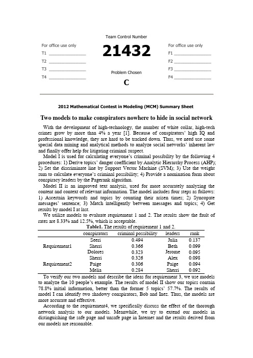
For office use onlyT1________________ T2________________ T3________________ T4________________Team Control Number21432Problem ChosenCFor office use onlyF1________________F2________________F3________________F4________________2012 Mathematical Contest in Modeling (MCM) Summary SheetTwo models to make conspirators nowhere to hide in social network With the development of high-technology, the number of white collar, high-tech crimes grow by more than 4% a year [1]. Bec ause of conspirators’ high IQ and professional knowledge, they are hard to be tracked down. Thus, we need use some special data mining and analytical methods to analyze social networks’ inherent law and finally offer help for litigating criminal suspect.M odel I is used for calculating everyone’s criminal possibility by the following 4 procedures: 1) Derive topics’ danger coefficient by Ana lytic Hierarchy Process (AHP);2) Set the discriminate line by Support Vector Machine (SVM); 3) Use the weight sum to c alculate everyone’s criminal possibility; 4) Provide a nomination form about conspiracy leaders by the Pagerank algorithm.Model II is an improved text analysis, used for more accurately analyzing the content and context of relevant information. The model includes four steps as follows: 1) Ascertain keywords and topics by counting their arisen times; 2) Syncopate me ssages’ sentence; 3) Match intelligently between messages and topics; 4) Get results by model I at last.We utilize models to evaluate requirement 1 and 2. The results show the fault of rates are 8.33% and 12.5%, which is acceptable.Table1. The results of requirement 1 and 2.conspirators criminal possibility leaders rankRequirement1Seeri 0.494 Julia 0.137 Sherri 0.366 Beth 0.099 Dolores 0.323 Jerome 0.095Requirement2 Sherri 0.326 Alex 0.098 Paige 0.306 Paige 0.094 Melia 0.284 Sherri 0.092To verify our two models and describe the ideas for requirement 3, we use models to analyze the 10 people’s example. The results of model II sho w our topics contain 78.8% initial information, better than the former 5 topics’ 57.7%. The results of model I can identify two shadowy conspirators, Bob and Inez. Thus, the models are more accurate and effective.According to the requirement4, we specifically discuss the effect of the thorough network analysis to our models. Meanwhile, we try to extend our models in distinguishing the safe page and unsafe page in Internet and the results derived from our models are reasonable.Two models to make conspirators nowhere to hideTeam #13373February 14th ,2012ContentIntroduction (3)The Description of the Problem (3)Analysis (3)What is the goal of the Modeling effort? (4)Flow chart (4)Assumptions (5)Terms, Definitions and Symbols (5)Model I (6)Overview (6)Model Built (6)Solution and Result (9)Analysis of the Result (10)Model II (11)Overview (11)Model Built (11)Result and Analysis (12)Conclusions (13)Technical summary (13)Strengths and Weaknesses (13)Extension (14)Reference (14)Appendix (16)IntroductionWith the development of our society, more and more high-tech conspiracy crimes and white-collar crimes take place in business and government professionals. Unlike simple violent crime, it is a kind of bran-new crime style, would gradually create big fraud schemes to hurt others’ benefit and destroy business companies.In order to track down the culprits and stop scams before they start, we must make full use of effective simulation model and methodology to search their criminal information. We create a Criminal Priority Model (CPM) to evaluate every suspect’s criminal possibility by analyzing text message and get a priority line which is helpful to ICM’s investigation.In addition, using semantic network analysis to search is one of the most effective ways nowadays; it will also be helpful we obtain and analysis semantic information by automatically extract networks using co-occurrence, grammatical analysis, and sentiment analysis. [1]During searching useful information and data, we develop a whole model about how to effective search and analysis data in network. In fact, not only did the coalescent of text analysis and disaggregated model make a contribution on tracking down culprits, but also provide an effective way for analyzing other subjects. For example, we can utilize our models to do the classification of pages.In fact, the conditions of pages’classification are similar to criminological analysis. First, according to the unsafe page we use the network crawler and Hyperlink to find the pages’ content and the connection between each pages. Second, extract the messages and the relationships between pages by Model II. Third, according to the available information, we can obtain the pages’priority list about security and the discriminate line separating safe pages and the unsafe pages by Model I. Finally we use the pages’ relationships to adjust the result.The Description of the ProblemAnalysisAfter reading the whole ICM problem, we make a depth analysis about the conspiracy and related information. In fact, the goal of ICM leads us to research how to take advantage of the thorough network, semantic, and text analyses of the message contents to work out personal criminal possibility.At first, we must develop a simulation model to analysis the current case’s data, and visualize the discriminate line of separating conspirator and non-conspirator.Then, by increasing text analyses to research the possible useful information from “Topic.xls”, we can optimize our model and develop an integral process of automatically extract and operate database.At last, use a new subject and database to verify our improved model.What is the goal of the Modeling effort?●Making a priority list for crime to present the most likely conspirators●Put forward some criteria to discriminate conspirator and non-conspirator, createa discriminate line.●Nominate the possible conspiracy leaders●Improve the model’s accuracy and the credit of ICM●Study the principle and steps of semantic network analysis●Describe how the semantic network analysis could empower our model.Flow chartFigure 1Assumptions●The messages have no serious error.●These messages and text can present what they truly mean.●Ignore special people, such as spy.●This information provided by ICM is reasonable and reliable.Terms, Definitions and SymbolsTable 2. Model parametersParameter MeaningThe rate of sending message to conspirators to total sending messageThe rate of receiving message to conspirators to total receiving messageThe dangerous possibility of one’s total messagesThe rate of messages with known non-conformist to total messagesDanger coefficient of topicsThe number of one’s sending messagesThe number of one’s receiving messagesThe number of one’s sending messages from criminalThe number of one’s receiving messages from criminalThe number of one’s sending messages from non-conspiratorThe number of one’s receiving messages from non-conspiratorDanger coefficient of peopleModel IOverviewModel I is used for calculating and analyzing everyone’s criminal possibility. In fact, the criminal possibility is the most important parameter to build a priority list and a discriminate line. The model I is made up of the following 4 procedures: (1) Derive topics’danger coefficient by Analytic Hierarchy Process (AHP); (2) Set the discriminate line by Support Vector Machine (SVM); (3) Use the weight sum to calculate everyone’s criminal possibility; (4) Provide a nomination form about conspiracy leaders by the Pagerank algorithm.Model BuiltStep.1PretreatmentIn order to decide the priority list and discriminate line, we must sufficiently study the data and factors in the ICM.For the first, we focus on the estimation about the phenomena of repeated names. In the name.xls, there are three pair phenomena of repeated names. Node#7 and node#37 both call Elsie, node#16 and node#34 both call Jerome, node#4 and node#32 both calls Gretchen. Thus, before develop simulation models; we must evaluate who are the real Elsie, Jerome and Gretchen.To decide which one accord with what information the problem submitsFirst we study the data in message.xls ,determine to analysis the number of messages of Elsie, Jerome and Gretchen. Table1 presents the correlation measure of their messages with criminal topic.Figure2By studying these data and figures, we can calculate the rate of messages about criminal topic to total messages; node#7 is 0.45455, while node#37 is 0.27273. Furthermore node#7 is higher than node#37 in the number of messages.Thus, we evaluate that node #7 is more likely Elsie what the ICM points out.In like manner, we think node#34, node#32 are those senior managers the ICM points out. In the following model and deduction, we assume node#7 is Elsie, node#34 is Jerome and node #32 is Gretchen.Step.2Derive topics’ danger coefficient by Analytic Hierarchy ProcessUse analytic hierarchy process to calculate the danger every topic’s coefficient. During the research, we decide use four factors’ effects to evaluate :● Aim :Evaluate the danger coefficient of every topic.[2]● Standard :The correlation with dangerous keywordsThe importance of the topic itselfThe relationship of the topic and known conspiratorsThe relationship of the topic and known non-conspirators● Scheme : The topics (1,2,3……15)Figure3According to previous research, we decide the weight of The Standard to Aim :These weights can be evaluated by paired comparison algorithm, and build a matrix about each part.For example, build a matrix about Standard and Aim, the equation is followingij j i a C C ⇒:ijji ij n n ij a a a a A 1,0)(=>=⨯ The other matrix can be evaluated by the similar ways. At last, we make a consistency check to matrix A and find it is reasonable.The result shows in the table, and we can use the data to continue the next model. Step.3 Use the weight sum to calculate everyone ’s criminal possibilityWe will start to study every one’s danger coefficient by using four factors,, and .[3]100-第一份工作开始时间)(第一份工作结束时间第一份工作持续时间=The first factor means calculate the rate of someone’s sending criminal messages to total sending messages.The second factors means calculate the rate of someone’s receivingcriminal messages to total receiving messages.=The third factormeans calculate the dangerous possibility of someone’stotal messages.The four factorthe rate of someone’s messages with non-conspirators tototal messages.At last, we use an equation to calculate every one’s criticality, namely thepossibility of someone attending crime. ( Shows every factors’weighing parameter)After calculating these equations abov e, we derive everyone’s criminal possibilityand a priority list. (See appendix for complete table about who are the most likely conspirators) We instead use a cratering technique first described by Rossmo [1999]. The two-dimensional crime points xi are mapped to their radius from the anchor point ai, that is, we have f : xi → ri, where f(xi) = j i i a a (a shifted modulus). The set ri isthen used to generate a crater around the anchor point.There are two dominatingStep.4 Provide a nomination form about conspiracy leaders by the Pagerankalgorithm.At last, we will find out the possible important leaders by pagerank model, and combined with priority list to build a prior conspiracy leaders list.[4]The essential idea from Page Rank is that if node u has a link to node v, then the author of u is an implicitly conferring some importance to node v. Meanwhile it means node v has a important chance. Thus, using B (u) to show the aggregation of links to node u, and using F (u) to show the aggregation of received links of node u, The C is Normalization factor. In each iteration, propagate the ranks as follows: The next equation shows page rank of node u:Using the results of Page Rank and priority list, we can know those possiblecriminal conspiracy leaders.Solution and ResultRequirement 1:According to Model I above, we calculate these data offered by requirement 1 and build two lists. The following shows the result of requirement 1.By running model I step2, we derive danger coefficient of topics, the known conspiracy topic 7, 11 and 13 are high danger coefficient (see appendix Table4. for complete information).After running model step3, we get a list of every one’s criticality .By comparing these criticality, we can build a priority list about criminal suspects. In fact, we find out criminal suspects are comparatively centralized, who are highly different from those known non-conspirators. This illuminates our model is relative reasonable. Thus we decide use SVM to get the discriminate line, namely to separate criminal suspects and possible non-conspirators (see appendix Table5. for complete information). Finally, we utilize Page rank to calculate criminal suspects’ Rank and status, table4 shows the result. Thus, we nominate 5 most likely criminal leaders according the results of table4.They are Julia, Beth, Jerome, Stephanie and Neal.According to the requirement of problem1, we underscore the situations of three senior managers Jerome, Delores and Gretchen. Because the SVM model makes a depth analysis about conspirators, Jerome is chosen as important conspirator, Delores and Gretchen both has high danger coefficient. We think Jerome could be a conspirator, while Delores and Gretchen are regarded as important criminal suspects. Using the software Ucinet, we derive a social network of criminal suspects.The blue nodes represent non-conspirators. The red nodes represent conspirators. The yellow nodes represent conspiracy leaders.Figure 4Requirement 2:Using the similar model above, we can continue analyzing the results though theconditions change.We derive three new tables (4, 5 and 6): danger coefficient of topics, every one’s criticality and the probability of nominated. At last, we get a new priority list (table6) and 5 most likely criminal leaders: Alex, Sherri, Yao, Elsie and Jerome.We sincerely wish that our analysis can be helpful to ICM’s investigation. We figure out a new figure, which shows the social network of criminal suspects for requirement 2.Figure 5Analysis of the Result1)AnalysisIn the requirement 1, we find out 24 possible criminal suspects. All of 7 known conspirators are in the 24 suspects and their danger coefficients are also pretty high. However, there are 2 known non-conspirators are in these suspects.Thus, the rate of making mistakes is 8.33%. In all, we still have enough reasons to think the model is reasonable.In addition, we find 5 suspects who are likely conspirators by Support Vector Machine (SVM).In the requirement 2, we also choose 24 the most likely conspirators after run our CPM. All of 8 known conspirators are also in the 24 suspects and their danger coefficients are pretty high. Because 3 known non-conspirators are in these suspects, the rate of making mistakes is 12.5%, which is higher to the result of requirement 1.2)ComparisonTo research the effect of changing the number of criminal topics and conspirators to results, we decide to do an additional research about their effect.We separate the change of topics and crimes’numbers, analysis result’s changes of only one factor:In order to analyze the change between requirement 1 and 2, we choose those people whose rank has a big change over 30.Reference: the node.1st result: the part of the requirement1’s priority list.2nd result: the part of the requirement2’s priority list.3rd result: the priority’s changes of requirement 1 and 2.After investigate these people, we find out the topics about them isn’t close connected with node#0. Thus, the change of node#0 does not make a great effect on their change.However, there are more than a half of people who talk about topic1. According to the analysis, we find the topic1 has a great effect on their change. The topic1 is more important to node#0.Thus; we can do an assumption that the decision of topics has bigger effect on the decision of the personal identity and decide to do a research in the following content.Model IIOverviewAccording to requirement3, we will take the text analysis into account to enhance our model. In the paper, text analysis is presented as a paradigm for syntactic-semantic analysis of natural language. The main characteristics of this approach are: the vectors of messages about keywords, semanteme and question formation. In like manner, we need get three vectors of topics. Then, we utilize similarity to separate every message to corresponding topics. Finally, we evaluate these effects of text analysis by model I.Model BuiltStep.1PretreatmentIn this step, we need conclude relatively accurate topics by keywords in messages. Not only builds a database about topics, but also builds a small database for adjusting the topic classification of messages. The small database for adjusting is used for studying possible interpersonal relation between criminal suspects, i. e. Bob always use positive and supportive words to comment topics and things about Jerry, and then we think Bob’s messages are closely connected with topics about Jerry. [5] At first, we need to count up how many keywords in the whole messages.Text analysis is word-oriented, i.e., the word plays the central role in language understanding. So we avoid stipulating a grammar in the traditional sense and focus on the concept of word. During the analysis of all words in messages, we ignore punctuation, some simple word such as “is” and “the”, and extract relative importantwords.Then, a statistics will be completed about how many times every important word occurs. We will make a priority list and choose the top part of these words.Finally, according to some messages, we will turn these keywords into relatively complete topics.Step.2Syncopate sentenceWe will make a depth research to every sentence in messages by running program In the beginning, we can utilize the same way in step1 to syncopate sentence, deriving every message’s keywords. We decide create a vector about keywords: = () (m is the number keywords in everymessage)For improving the accuracy and relativity of our keywords, we decide to build a vector that shows every keyword’s synonyms, antonym.= () (1<k<m, p is the number of correlative words)According to primary analysis, we can find some important interpersonal relations between criminal suspects, i.e. Bob is closely connected with Jerry, then we can build a vector about interpersonal relation.= () (n is the number of relationships in one sentence )Step.3Intelligent matchingIn order to improve the accuracy of our disaggregated model, we use three vectors to do intelligent matching.Every message has three vectors:. Similarly, every topic alsohas three vectors.At last, we can do an intelligent matching to classify. [6]Step.4Using CPMAfter deriving new the classification of messages, we will make full use of new topics to calculate every one’s criticality.Result and AnalysisAfter calculating the 10 people example, we derive new topics. By verifying the topics’ contained initial information, we can evaluate the effect of models.The results of model II show our topics contain 78.8% initial information, better than former 5 topics’ 57.7%.T hus, new topics contain more initial information. Meanwhile, we build a database about interpersonal relation, and using it to optimize the results of everyone’s criminal possibility.Table 3#node primary new #node primary new1 0 0.065 6 0.342 0.2652 0.342 0.693 7 0.891 0.9123 0.713 0.562 8 0.423 0.354 1 1 9 0.334 0.7235 0.823 0.853 10 0.125 0.15 The results of model I can identify the two shadowy conspirators, Bob and Inez. In the table, the rate of fault is becoming smaller.According to Table11, we can derive some information:1.Analysis the danger coefficient of two people, Bob and Inez. Bob is theperson who self-admitted his involvement in a plan bargain for a reducedsentence. His data changes from 0.342 to 0.693. And Inez is the person whogot off, his data changes from 0.334 to 0.723. The models can identify thetwo shadowy people.2.Carol, the person who was later dropped his data changes from 0.713 to0.562. Although it still has a relatively high danger coefficient, the resultsare enhancing by our models.3.The distance between high degree people and low degree become bigger, itpresents the models would more distinctly identify conspirators andnon-conspirators.Thus, the models are more accurate and effective.ConclusionsTechnical summaryWe bring out a whole model about how to extract and analysis plentiful network information, and finally solve the classification problems. Four steps are used to make the classification problem easier.1)According known conspirators and correlative information, use resemblingnetwork crawler to extract what we may need information and messages.[7]2)Using the second model to analysis and classify these messages and text, getimportant topics.3)Using the first model to calculate everyone’s criminal possibility.4)Using an interpersonal relation database derived by step2 to optimize theresults. [8]Strengths and WeaknessesStrengths:1)We analyze the danger coefficient of topics and people by using different characteristics to describe them. Its results have a margin of error of 10percentage points. That the Models work well.2)In the semantic analysis, in addition to obtain topics from messages in social network, we also extract the relationships of people and adjust the final resultimprove the model.3)We use 4 characteristics to describe people’s danger coefficient. SVM has a great advantage in classification by small characteristics. Using SVM to classify the unknown people and its result is good.Weakness:1)For the special people, such as spy and criminal researcher, the model works not so well.2)We can determine some criminals by topics; at the same time we can also use the new criminals to adjust the topics. The two react upon each other. We canexpect to cycle through several times until the topics and criminals are stable.However we only finish the first cycle.3)For the semantic analysis model we have established, we just test and verify in the example (social network of 10 people). In the condition of large social network, the computational complexity will become greater, so the classify result is still further to be surveyed.ExtensionAccording to our analysis, not only can our model be applied to analyze criminal gangs, but also applied to similar network models, such as cells in a biological network, safe pages in Internet and so on. For the pages’ classification in Internet, our model would make a contribution. In the following, we will talk about how to utilize [9] Our model in pages’ classification.First, according to the unsafe page we use the network crawler and Hyperlink to find the pages’content and the connection between each page. Second, extract the messages and the relationships between pages by Model II. Third, according to the available information, we can obtain the pages’priority list about security and the discriminate line separating safe pages and the unsafe pages by Model I. Finally we use the pages’ relationships to adjust the result.Reference1. http://books.google.pl/books?id=CURaAAAAYAAJ&hl=zh-CN2012.2. AHP./wiki/%E5%B1%82%E6%AC%A1%E5%88%86%E6%9E%90%E6%B 3%95.3. Schaller, J. and J.M.S. Valente, Minimizing the weighted sum of squared tardiness on a singlemachine. Computers & Operations Research, 2012. 39(5): p. 919-928.4. Frahm, K.M., B. Georgeot, and D.L. Shepelyansky, Universal emergence of PageRank.Journal of Physics a-Mathematical and Theoretical, 2011. 44(46).5. Park, S.-B., J.-G. Jung, and D. Lee, Semantic Social Network Analysis for HierarchicalStructured Multimedia Browsing. Information-an International Interdisciplinary Journal, 2011.14(11): p. 3843-3856.6. Yi, J., S. Tang, and H. Li, Data Recovery Based on Intelligent Pattern Matching.ChinaCommunications, 2010. 7(6): p. 107-111.7. Nath, R. and S. Bal, A Novel Mobile Crawler System Based on Filtering off Non-ModifiedPages for Reducing Load on the Network.International Arab Journal of Information Technology, 2011. 8(3): p. 272-279.8. Xiong, F., Y. Liu, and Y. Li, Research on Focused Crawler Based upon Network Topology.Journal of Internet Technology, 2008. 9(5): p. 377-380.9. Huang, D., et al., MyBioNet: interactively visualize, edit and merge biological networks on theWeb. Bioinformatics, 2011. 27(23): p. 3321-3322.AppendixTable 4requirement 1topic danger topic danger topic danger topic danger7 1.65 4 0.78 5 0.47 8 0.1713 1.61 10 0.77 15 0.46 14 0.1711 1.60 12 0.47 9 0.19 6 0.141 0.812 0.473 0.18requirement 2topic danger topic danger topic danger topic danger1 0.402 0.26 15 0.15 14 0.117 0.37 9 0.23 8 0.15 3 0.0913 0.37 10 0.21 5 0.14 6 0.0611 0.30 12 0.18 4 0.12Table 5requirement 1#node danger #node danger #node danger #node danger 21 0.74 22 0.19 0 0.13 23 0.03 67 0.69 4 0.19 40 0.13 72 0.03 54 0.61 33 0.19 36 0.13 62 0.03 81 0.49 47 0.19 11 0.12 51 0.02 7 0.47 41 0.19 69 0.12 57 0.02 3 0.37 28 0.18 29 0.12 64 0.02 49 0.36 16 0.18 12 0.11 71 0.02 43 0.36 31 0.17 25 0.11 74 0.01 10 0.32 37 0.17 82 0.11 58 0.01 18 0.29 27 0.16 60 0.10 59 0.01 34 0.29 45 0.16 42 0.10 70 0.00 48 0.28 50 0.16 65 0.09 53 0.00 20 0.27 24 0.16 9 0.09 76 0.00 15 0.27 44 0.16 5 0.09 61 0.00 17 0.26 38 0.16 66 0.09 75 -0.01 2 0.23 13 0.16 26 0.08 77 -0.01 32 0.23 35 0.15 39 0.06 55 -0.02 30 0.20 1 0.15 80 0.04 68 -0.02 73 0.20 46 0.15 78 0.04 52 -0.0319 0.20 8 0.14 56 0.03 63 -0.03 14 0.19 6 0.14 79 0.03requirement 2#node danger #node danger #node danger #node danger 0 0.39881137 75 0.1757106 47 0.1090439 11 0.0692506 21 0.447777778 52 0.1749354 71 0.1089147 4 0.0682171 67 0.399047158 38 0.1738223 82 0.1088594 42 0.0483204 54 0.353754153 10 0.1656977 14 0.1079734 65 0.046124 81 0.325736434 19 0.1559173 27 0.1060724 60 0.0459948 2 0.306054289 40 0.1547065 23 0.105814 39 0.0286822 18 0.303178295 30 0.1517626 5 0.1039406 62 0.0245478 66 0.28372093 80 0.145155 8 0.10228 78 0.0162791 7 0.279870801 24 0.1447674 73 0.1 56 0.0160207 63 0.261886305 70 0.1425711 50 0.0981395 64 0.0118863 68 0.248514212 29 0.1425562 26 0.097213 72 0.011369548 0.239668277 45 0.1374667 1 0.0952381 79 0.009302349 0.238076781 37 0.1367959 69 0.0917313 51 0.0056848 34 0.232614868 17 0.1303064 33 0.0906977 57 0.0056848 3 0.225507567 6 0.1236221 31 0.0905131 74 0.0054264 35 0.222435188 22 0.1226934 36 0.0875452 76 0.005168 77 0.214470284 13 0.1222868 41 0.0822997 53 0.0028424 20 0.213718162 44 0.115007 46 0.0749354 58 0.0015504 43 0.204328165 12 0.1121447 28 0.0748708 59 0.0015504 32 0.193311469 15 0.1121447 16 0.074234 61 0.0007752 55 0.182687339 9 0.1117571 25 0.0701292Table 6requirement 1#node leader #node leader #node leader #node leader 15 0.1368 49 0.0481 7 0.0373 19 0.0089 14 0.0988 4 0.0423 21 0.0357 32 0.0073 34 0.0951 10 0.0422 18 0.029 22 0.0059 30 0.0828 67 0.0421 48 0.0236 81 0.0053 17 0.0824 54 0.0377 20 0.0232 73 043 0.0596 3 0.0377 2 0.0181 33 0requirement 2#node leader #node leader #node leader #node leader 21 0.0981309 7 0.0714406 54 0.0526831 43 0.01401872 0.0942899 34 0.0707246 32 0.0464614 81 0.00977763 0.0916127 0 0.0706746 18 0.041114248 0.0855984 20 0.0658119 68 0.028532867 0.0782211 49 0.0561665 35 0.024741。
美赛论文模版
摘要:第一段:写论文解决什么问题1.问题的重述a. 介绍重点词开头:例1:“Hand move” irrigation, a cheap but labor-intensive system used on small farms, consists of a movable pipe with sprinkler on top that can be attached to a stationary main.例2:……is a real-life common phenomenon with many complexi t ies.例3:An (effective plan) is crucial to………b. 直接指出问题:例1:We find the optimal number of tollbooths in a highway toll-plaza for a given number of highway lanes: the number of tollbooths that minimizes average delay experienced by cars.例2:A brand-new university needs to balance the cost of information technology security measures wi t h the potential cost of attacks on its systems.例3:We determine the number of sprinklers to use by analyzing the energy and motion of water in the pipe and examining the engineering parameters of sprinklers available in the market.例4: After mathematically analyzing the …… problem, our modeling group would like to present our conclusions, strategies, (and recommendations )to the …….例5:Our goal is... that (mini mizes the time )……….2.解决这个问题的伟大意义反面说明。
美赛金奖论文
1
Team # 14604
Catalogue
Abstracts ........................................................................................................................................... 1 Contents ............................................................................................................................................ 3 1. Introduction ................................................................................................................................... 3 1.1 Restatement of the Problem ................................................................................................ 3 1.2 Survey of the Previous Research......................................................................................... 3 2. Assumptions .................................................................................................................................. 4 3. Parameters ..................................................................................................................................... 4 4. Model A ----------Package model .................................................................................................. 6 4.1 Motivation ........................................................................................................................... 6 4.2 Development ....................................................................................................................... 6 4.2.1 Module 1: Introduce of model A .............................................................................. 6 4.2.2 Module 2: Solution of model A .............................................................................. 10 4.3 Conclusion ........................................................................................................................ 11 5. Model B----------Optional model ................................................................................................ 12 5.1 Motivation ......................................................................................................................... 12 5.2 Development ..................................................................................................................... 12 5.2.1 Module B: Choose oar- powered rubber rafts or motorized boats either ............... 12 5.2.2 Module 2: Choose mix of oar- powered rubber rafts and motorized boats ............ 14 5.3 Initial arrangement ............................................................................................................ 17 5.4. Deepened model B ........................................................................................................... 18 5.4.1 Choose the campsites allodium .............................................................................. 18 5.4.2 Choose the oar- powered rubber rafts or motorized boats allodium ...................... 19 5.5 An example of reasonable arrangement ............................................................................ 19 5.6 The strengths and weakness .............................................................................................. 20 6. Extensions ................................................................................................................................... 21 7. Memo .......................................................................................................................................... 25 8. References ................................................................................................................................... 26 9. Appendices .................................................................................................................................. 27 9.1 Appendix I .................................................................................................. 27 9.2 Appendix II ....................................................................................................................... 29
美赛一等奖论文-中文翻译版
目录问题回顾 (3)问题分析: (4)模型假设: (6)符号定义 (7)4.1---------- (8)4.2 有热水输入的温度变化模型 (17)4.2.1模型假设与定义 (17)4.2.2 模型的建立The establishment of the model (18)4.2.3 模型求解 (19)4.3 有人存在的温度变化模型Temperature model of human presence (21)4.3.1 模型影响因素的讨论Discussion influencing factors of the model (21)4.3.2模型的建立 (25)4.3.3 Solving model (29)5.1 优化目标的确定 (29)5.2 约束条件的确定 (31)5.3模型的求解 (32)5.4 泡泡剂的影响 (35)5.5 灵敏度的分析 (35)8 non-technical explanation of the bathtub (37)Summary人们经常在充满热水的浴缸里得到清洁和放松。
本文针对只有一个简单的热水龙头的浴缸,建立一个多目标优化模型,通过调整水龙头流量大小和流入水的温度来使整个泡澡过程浴缸内水温维持基本恒定且不会浪费太多水。
首先分析浴缸中水温度变化的具体情况。
根据能量转移的特点将浴缸中的热量损失分为两类情况:沿浴缸四壁和底面向空气中丧失的热量根据傅里叶导热定律求出;沿水面丧失的热量根据水由液态变为气态的焓变求出。
因涉及的参数过多,将系数进行回归分析的得到一个一元二次函数。
结合两类热量建立了温度关于时间的微分方程。
加入阻滞因子考虑环境温湿度升高对水温的影响,最后得到水温度随时间的变化规律(见图**)。
优化模型考虑保持水龙头匀速流入热水的情况。
将过程分为浴缸未加满和浴缸加满而水从排水口溢出的两种情况,根据能量守恒定律优化上述微分方程,建立一个有热源的情况下水的温度随时间变化的分段模型,(见图**)接下来考虑人在浴缸中对水温的影响。
2012美国数学建模大赛二等奖论文及格式——英文版
Dedicated Pipeline for Trip ArrangementSummaryIn the problem of camping, we should set reasonable schedule which can not only increase the utilization of campsites but also meet people's needs. Meanwhile, the carrying capacity of the river is also required. To solve the problem, this thesis will build optimization model with maximum campsite's utilization and river trips as the model's target function.The specific steps are as follows:step1: Determine the number of campsites Y. We use Computer Emulation Simulation to solve this problem by making full use of the given conditions that trips will spend6 to 18 nights on the river and the river is 225 miles long. We get 29 sets of data through programming, then curve fitting them by SPSS software. By comparing the value of sig. and adjusting R square and so on, the ideal number of the campsites is got .Step2: By using the number of the campsites 39 as well as the goal programming equation built in the first step, we get the number of river trips that are allowed to enter, namely the carrying capacity of the river.Step3: By using the campsites 39, we adjust the campsites of different camping program and then divide them into 4 kinds through clustering analysis using SPSS. Then we select representatives in various types of camping programs according to repetition rate and the average transfer rate. So we streamline the camping programs into the problem of goal programming for 6, 8, 11, 12, 16 nights.Step4: In those five camping programs, 39 campsites which will not repeat are distributed in 3 dedicated pipelines . The first line accounts for 12 campsites and can only be available for 6 or 12 nights trip. Each day, a couple of 6 nights trips are distributed, and the starting trip camps the campsites in turn according to the even number of the pipeline while the secondary trip camps in turn according to the odd number. The second pipeline accounting for 16 campsites is arranged just as the first one .Under the premise of guaranteeing the variety of camping project, trips start as a pipeline to make the total number of trips camping in this line the biggest and the utilization of the campsites maximum. There are 11 campsites in the third pipeline which are available for 6 to 11 nights trip.According to the above analysis, the carrying capacity of Dedicated Pipeline, namely C_line, is less than that of the river, namely C_river, within 180 days. the park managers need to grasp passenger flow(P) of the river in the following period(T) and calculate P/( C_line/T)The best distribution program: the best utirlization of campsites is P/( C_line/T) in one period.According to the best utilization of campsites, The best distribution program can be got.Key words: Cluster Analysis, Bus Rapid, Transit Pipeline System, Curve Fitting , Computer Emulation SimulationContentsI. Introduction (3)1.1Restatement of the problem (3)1.2 Theory knowledge introduction (3)II. Definitions and Key terms (4)1,The conditions given (4)2,Symbol definition (4)III. General Assumptions (4)IV Model Design (5)4.1Model Establishment (5)4.2 Model Solution (6)4.2.1.To determine Y (6)4.2.1 To Determine the Camping program (11)4.2.3 To find capacity of the river (15)4.2.3 Determine Dedicated Pipeline (15)4.3 Strength and Weakness............................................................. 错误!未定义书签。
美赛数学建模比赛论文实用模板
The Keep-Right-Except-To-Pass RuleSummaryAs for the first question, it provides a traffic rule of keep right except to pass, requiring us to verify its effectiveness. Firstly, we define one kind of traffic rule different from the rule of the keep right in order to solve the problem clearly; then, we build a Cellular automaton model and a Nasch model by collecting massive data; next, we make full use of the numerical simulation according to several influence factors of traffic flow; At last, by lots of analysis of graph we obtain, we indicate a conclusion as follow: when vehicle density is lower than 0.15, the rule of lane speed control is more effective in terms of the factor of safe in the light traffic; when vehicle density is greater than 0.15, so the rule of keep right except passing is more effective In the heavy traffic.As for the second question, it requires us to testify that whether the conclusion we obtain in the first question is the same apply to the keep left rule. First of all, we build a stochastic multi-lane traffic model; from the view of the vehicle flow stress, we propose that the probability of moving to the right is 0.7and to the left otherwise by making full use of the Bernoulli process from the view of the ping-pong effect, the conclusion is that the choice of the changing lane is random. On the whole, the fundamental reason is the formation of the driving habit, so the conclusion is effective under the rule of keep left.As for the third question, it requires us to demonstrate the effectiveness of the result advised in the first question under the intelligent vehicle control system. Firstly, taking the speed limits into consideration, we build a microscopic traffic simulator model for traffic simulation purposes. Then, we implement a METANET model for prediction state with the use of the MPC traffic controller. Afterwards, we certify that the dynamic speed control measure can improve the traffic flow .Lastly neglecting the safe factor, combining the rule of keep right with the rule of dynamical speed control is the best solution to accelerate the traffic flow overall.Key words:Cellular automaton model Bernoulli process Microscopic traffic simulator model The MPC traffic controlContentContent (2)1. Introduction (3)2. Analysis of the problem (3)3. Assumption (3)4. Symbol Definition (3)5. Models (4)5.1 Building of the Cellular automaton model (4)5.1.1 Verify the effectiveness of the keep right except to pass rule (4)5.1.2 Numerical simulation results and discussion (5)5.1.3 Conclusion (8)5.2 The solving of second question (8)5.2.1 The building of the stochastic multi-lane traffic model (9)5.2.2 Conclusion (9)5.3 Taking the an intelligent vehicle system into a account (9)5.3.1 Introduction of the Intelligent Vehicle Highway Systems (9)5.3.2 Control problem (9)5.3.3 Results and analysis (9)5.3.4 The comprehensive analysis of the result (10)6. Improvement of the model (11)6.1 strength and weakness (11)6.1.1 Strength (11)6.1.2 Weakness (11)6.2 Improvement of the model (11)7. Reference (13)1. IntroductionAs is known to all, it’s essential for us to drive automobiles, thus the driving rules is crucial important. In many countries like USA, China, drivers obey the rules which called “The Keep-Right-Except-To-Pass (that is, when driving automobiles, the rule requires drivers to drive in the right-most unless theyare passing another vehicle)”.2. Analysis of the problemFor the first question, we decide to use the Cellular automaton to build models,then analyze the performance of this rule in light and heavy traffic. Firstly,we mainly use the vehicle density to distinguish the light and heavy traffic; secondly, we consider the traffic flow and safe as the represent variable which denotes the light or heavy traffic; thirdly, we build and analyze a Cellular automaton model; finally, we judge the rule through two different driving rules,and then draw conclusions.3. AssumptionIn order to streamline our model we have made several key assumptions●The highway of double row three lanes that we study can representmulti-lane freeways.●The data that we refer to has certain representativeness and descriptive●Operation condition of the highway not be influenced by blizzard oraccidental factors●Ignore the driver's own abnormal factors, such as drunk driving andfatigue driving●The operation form of highway intelligent system that our analysis canreflect intelligent system●In the intelligent vehicle system, the result of the sampling data hashigh accuracy.4. Symbol Definitioni The number of vehiclest The time5. ModelsBy analyzing the problem, we decided to propose a solution with building a cellular automaton model.5.1 Building of the Cellular automaton modelThanks to its simple rules and convenience for computer simulation, cellular automaton model has been widely used in the study of traffic flow in recent years. Let )(t x i be the position of vehicle i at time t , )(t v i be the speed of vehicle i at time t , p be the random slowing down probability, and R be the proportion of trucks and buses, the distance between vehicle i and the front vehicle at time t is:1)()(1--=-t x t x gap i i i , if the front vehicle is a small vehicle.3)()(1--=-t x t x gap i i i , if the front vehicle is a truck or bus.5.1.1 Verify the effectiveness of the keep right except to pass ruleIn addition, according to the keep right except to pass rule, we define a new rule called: Control rules based on lane speed. The concrete explanation of the new rule as follow:There is no special passing lane under this rule. The speed of the first lane (the far left lane) is 120–100km/h (including 100 km/h);the speed of the second lane (the middle lane) is 100–80km8/h (including80km/h);the speed of the third lane (the far right lane) is below 80km/ h. The speeds of lanes decrease from left to right.● Lane changing rules based lane speed controlIf vehicle on the high-speed lane meets control v v <, ),1)(min()(max v t v t gap i f i +≥, safe b i gap t gap ≥)(, the vehicle will turn into the adjacent right lane, and the speed of the vehicle after lane changing remains unchanged, where control v is the minimum speed of the corresponding lane.● The application of the Nasch model evolutionLet d P be the lane changing probability (taking into account the actual situation that some drivers like driving in a certain lane, and will not takethe initiative to change lanes), )(t gap f i indicates the distance between the vehicle and the nearest front vehicle, )(t gap b i indicates the distance between the vehicle and the nearest following vehicle. In this article, we assume that the minimum safe distance gap safe of lane changing equals to the maximum speed of the following vehicle in the adjacent lanes.Lane changing rules based on keeping right except to passIn general, traffic flow going through a passing zone (Fig. 5.1.1) involves three processes: the diverging process (one traffic flow diverging into two flows), interacting process (interacting between the two flows), and merging process (the two flows merging into one) [4].Fig.5.1.1 Control plan of overtaking process(1) If vehicle on the first lane (passing lane) meets ),1)(min()(max v t v t gap i f i +≥ and safe b i gap t gap ≥)(, the vehicle will turn into the second lane, the speed of the vehicle after lane changing remains unchanged.5.1.2 Numerical simulation results and discussionIn order to facilitate the subsequent discussions, we define the space occupation rate as L N N p truck CAR ⨯⨯+=3/)3(, where CAR N indicates the number ofsmall vehicles on the driveway,truck N indicates the number of trucks and buses on the driveway, and L indicates the total length of the road. The vehicle flow volume Q is the number of vehicles passing a fixed point per unit time,T N Q T /=, where T N is the number of vehicles observed in time duration T .The average speed ∑∑⨯=T it i a v T N V 11)/1(, t i v is the speed of vehicle i at time t . Take overtaking ratio f p as the evaluation indicator of the safety of traffic flow, which is the ratio of the total number of overtaking and the number of vehicles observed. After 20,000 evolution steps, and averaging the last 2000 steps based on time, we have obtained the following experimental results. In order to eliminate the effect of randomicity, we take the systemic average of 20 samples [5].Overtaking ratio of different control rule conditionsBecause different control conditions of road will produce different overtaking ratio, so we first observe relationships among vehicle density, proportion of large vehicles and overtaking ratio under different control conditions.(a) Based on passing lane control (b) Based on speed control Fig.5.1.3Fig.5.1.3 Relationships among vehicle density, proportion of large vehicles and overtaking ratio under different control conditions.It can be seen from Fig. 5.1.3:(1) when the vehicle density is less than 0.05, the overtaking ratio will continue to rise with the increase of vehicle density; when the vehicle density is larger than 0.05, the overtaking ratio will decrease with the increase of vehicle density; when density is greater than 0.12, due to the crowding, it willbecome difficult to overtake, so the overtaking ratio is almost 0.(2) when the proportion of large vehicles is less than 0.5, the overtaking ratio will rise with the increase of large vehicles; when the proportion of large vehicles is about 0.5, the overtaking ratio will reach its peak value; when the proportion of large vehicles is larger than 0.5, the overtaking ratio will decrease with the increase of large vehicles, especially under lane-based control condition s the decline is very clear.● Concrete impact of under different control rules on overtaking ratioFig.5.1.4Fig.5.1.4 Relationships among vehicle density, proportion of large vehicles and overtaking ratio under different control conditions. (Figures in left-hand indicate the passing lane control, figures in right-hand indicate the speed control. 1f P is the overtaking ratio of small vehicles over large vehicles, 2f P is the overtaking ratio of small vehicles over small vehicles, 3f P is the overtaking ratio of large vehicles over small vehicles, 4f P is the overtaking ratio of large vehicles over large vehicles.). It can be seen from Fig. 5.1.4:(1) The overtaking ratio of small vehicles over large vehicles under passing lane control is much higher than that under speed control condition, which is because, under passing lane control condition, high-speed small vehicles have to surpass low-speed large vehicles by the passing lane, while under speed control condition, small vehicles are designed to travel on the high-speed lane, there is no low- speed vehicle in front, thus there is no need to overtake.● Impact of different control rules on vehicle speedFig. 5.1.5 Relationships among vehicle density, proportion of large vehicles and average speed under different control conditions. (Figures in left-hand indicates passing lane control, figures in right-hand indicates speed control.a X is the average speed of all the vehicles, 1a X is the average speed of all the small vehicles, 2a X is the average speed of all the buses and trucks.).It can be seen from Fig. 5.1.5:(1) The average speed will reduce with the increase of vehicle density and proportion of large vehicles.(2) When vehicle density is less than 0.15,a X ,1a X and 2a X are almost the same under both control conditions.Effect of different control conditions on traffic flowFig.5.1.6Fig. 5.1.6 Relationships among vehicle density, proportion of large vehicles and traffic flow under different control conditions. (Figure a1 indicates passing lane control, figure a2 indicates speed control, and figure b indicates the traffic flow difference between the two conditions.It can be seen from Fig. 5.1.6:(1) When vehicle density is lower than 0.15 and the proportion of large vehicles is from 0.4 to 1, the traffic flow of the two control conditions are basically the same.(2) Except that, the traffic flow under passing lane control condition is slightly larger than that of speed control condition.5.1.3 ConclusionIn this paper, we have established three-lane model of different control conditions, studied the overtaking ratio, speed and traffic flow under different control conditions, vehicle density and proportion of large vehicles.5.2 The solving of second question5.2.1 The building of the stochastic multi-lane traffic model5.2.2 ConclusionOn one hand, from the analysis of the model, in the case the stress is positive, we also consider the jam situation while making the decision. More specifically, if a driver is in a jam situation, applying ))(,2(x P B R results with a tendency of moving to the right lane for this driver. However in reality, drivers tend to find an emptier lane in a jam situation. For this reason, we apply a Bernoulli process )7.0,2(B where the probability of moving to the right is 0.7and to the left otherwise, and the conclusion is under the rule of keep left except to pass, So, the fundamental reason is the formation of the driving habit.5.3 Taking the an intelligent vehicle system into a accountFor the third question, if vehicle transportation on the same roadway was fully under the control of an intelligent system, we make some improvements for the solution proposed by us to perfect the performance of the freeway by lots of analysis.5.3.1 Introduction of the Intelligent Vehicle Highway SystemsWe will use the microscopic traffic simulator model for traffic simulation purposes. The MPC traffic controller that is implemented in the Matlab needs a traffic model to predict the states when the speed limits are applied in Fig.5.3.1. We implement a METANET model for prediction purpose[14].5.3.2 Control problemAs a constraint, the dynamic speed limits are given a maximum and minimum allowed value. The upper bound for the speed limits is 120 km/h, and the lower bound value is 40 km/h. For the calculation of the optimal control values, all speed limits are constrained to this range. When the optimal values are found, they are rounded to a multiplicity of 10 km/h, since this is more clear for human drivers, and also technically feasible without large investments.5.3.3 Results and analysisWhen the density is high, it is more difficult to control the traffic, since the mean speed might already be below the control speed. Therefore, simulations are done using densities at which the shock wave can dissolve without using control, and at densities where the shock wave remains. For each scenario, five simulations for three different cases are done, each with a duration of one hour. The results of the simulations are reported in Table 5.1, 5.2, 5.3. Table.5.1 measured results for the unenforced speed limit scenariodem q case#1 #2 #3 #4 #5 TTS:mean(std ) TPN 4700no shock 494.7452.1435.9414.8428.3445.21(6.9%) 5:4wave 3 5 8 8 0 14700nocontrolled520.42517.48536.13475.98539.58517.92(4.9%)6:364700 controlled 513.45488.43521.35479.75-486.5500.75(4.0%)6:244700 no shockwave493.9472.6492.78521.1489.43493.96(3.5%)6:034700 uncontrolled635.1584.92643.72571.85588.63604.84(5.3%)7:244700 controlled 575.3654.12589.77572.15586.46597.84(6.4%)7:19●Enforced speed limits●Intelligent speed adaptationFor the ISA scenario, the desired free-flow speed is about 100% of the speed limit. The desired free-flow speed is modeled as a Gaussian distribution, with a mean value of 100% of the speed limit, and a standard deviation of 5% of the speed limit. Based on this percentage, the influence of the dynamic speed limits is expected to be good[19].5.3.4 The comprehensive analysis of the resultFrom the analysis above, we indicate that adopting the intelligent speed control system can effectively decrease the travel times under the control of an intelligent system, in other words, the measures of dynamic speed control can improve the traffic flow.Evidently, under the intelligent speed control system, the effect of the dynamic speed control measure is better than that under the lane speed control mentioned in the first problem. Because of the application of the intelligent speed control system, it can provide the optimal speed limit in time. In addition, it can guarantee the safe condition with all kinds of detection device and the sensor under the intelligent speed system.On the whole, taking all the analysis from the first problem to the end into a account, when it is in light traffic, we can neglect the factor of safe with the help of the intelligent speed control system.Thus, under the state of the light traffic, we propose a new conclusion different from that in the first problem: the rule of keep right except to pass is more effective than that of lane speed control.And when it is in the heavy traffic, for sparing no effort to improve the operation efficiency of the freeway, we combine the dynamical speed control measure with the rule of keep right except to pass, drawing a conclusion that the application of the dynamical speed control can improve the performance ofthe freeway.What we should highlight is that we can make some different speed limit as for different section of road or different size of vehicle with the application of the Intelligent Vehicle Highway Systems.In fact, that how the freeway traffic operate is extremely complex, thereby, with the application of the Intelligent Vehicle Highway Systems, by adjusting our solution originally, we make it still effective to freeway traffic.6. Improvement of the model6.1 strength and weakness6.1.1 Strength●it is easy for computer simulating and can be modified flexibly to consideractual traffic conditions ,moreover a large number of images make the model more visual.●The result is effectively achieved all of the goals we set initially, meantimethe conclusion is more persuasive because of we used the Bernoulli equation.●We can get more accurate result as we apply Matlab.6.1.2 Weakness●The relationship between traffic flow and safety is not comprehensivelyanalysis.●Due to there are many traffic factors, we are only studied some of the factors,thus our model need further improved.6.2 Improvement of the modelWhile we compare models under two kinds of traffic rules, thereby we come to the efficiency of driving on the right to improve traffic flow in some circumstance. Due to the rules of comparing is too less, the conclusion is inadequate. In order to improve the accuracy, We further put forward a kinds of traffic rules: speed limit on different type of cars.The possibility of happening traffic accident for some vehicles is larger, and it also brings hidden safe troubles. So we need to consider separately about different or specific vehicle types from the angle of the speed limiting in order to reduce the occurrence of traffic accidents, the highway speed limit signs is in Fig.6.1.Fig .6.1Advantages of the improving model are that it is useful to improve the running condition safety of specific type of vehicle while considering the difference of different types of vehicles. However, we found that the rules may be reduce the road traffic flow through the analysis. In the implementation it should be at the 85V speed of each model as the main reference basis. In recent years, the 85V of some researchers for the typical countries from Table 6.1[ 21]: Table 6.1 Operating speed prediction modeAuthorCountry Model Ottesen andKrammes2000America LC DC L DC V C ⨯---=01.0012.057.144.10285Andueza2000Venezuel a ].[308.9486.7)/894()/2795(25.9885curve horizontal L DC Ra R V T ++--= ].[tan 819.27)/3032(69.10085gent L R V T +-= Jessen2001 America ][00239.0614.0279.080.86185LSD ADT G V V P --+=][00212.0432.010.7285NLSD ADT V V P -+=Donnell2001 America 22)2(8500724.040.10140.04.78T L G R V --+=22)3(85008369.048.10176.01.75T L G R V --+= 22)4(8500810.069.10176.05.74T L G R V --+=22)5(8500934.008.21.83T L G V --=BucchiA.BiasuzziK.And SimoneA.2005Italy DC V 124.0164.6685-= DC E V 4.046.3366.5585--= 2855.035.1119.0745.65DC E DC V ---= Fitzpatrick America KV 98.17507.11185-= Meanwhile, there are other vehicles driving rules such as speed limit in adverseweather conditions. This rule can improve the safety factor of the vehicle to some extent. At the same time, it limits the speed at the different levels.7. Reference[1] M. Rickert, K. Nagel, M. Schreckenberg, A. Latour, Two lane traffi csimulations using cellular automata, Physica A 231 (1996) 534–550.[20] J.T. Fokkema, Lakshmi Dhevi, Tamil Nadu Traffi c Management and Control inIntelligent Vehicle Highway Systems,18(2009).[21] Yang Li, New Variable Speed Control Approach for Freeway. (2011) 1-66。
美赛数学建模比赛论文资料材料模板
The Keep-Right-Except-To-Pass RuleSummaryAs for the first question, it provides a traffic rule of keep right except to pass, requiring us to verify its effectiveness. Firstly, we define one kind of traffic rule different from the rule of the keep right in order to solve the problem clearly; then, we build a Cellular automaton model and a Nasch model by collecting massive data; next, we make full use of the numerical simulation according to several influence factors of traffic flow; At last, by lots of analysis of graph we obtain, we indicate a conclusion as follow: when vehicle density is lower than 0.15, the rule of lane speed control is more effective in terms of the factor of safe in the light traffic; when vehicle density is greater than 0.15, so the rule of keep right except passing is more effective In the heavy traffic.As for the second question, it requires us to testify that whether the conclusion we obtain in the first question is the same apply to the keep left rule. First of all, we build a stochastic multi-lane traffic model; from the view of the vehicle flow stress, we propose that the probability of moving to the right is 0.7and to the left otherwise by making full use of the Bernoulli process from the view of the ping-pong effect, the conclusion is that the choice of the changing lane is random. On the whole, the fundamental reason is the formation of the driving habit, so the conclusion is effective under the rule of keep left.As for the third question, it requires us to demonstrate the effectiveness of the result advised in the first question under the intelligent vehicle control system. Firstly, taking the speed limits into consideration, we build a microscopic traffic simulator model for traffic simulation purposes. Then, we implement a METANET model for prediction state with the use of the MPC traffic controller. Afterwards, we certify that the dynamic speed control measure can improve the traffic flow .Lastly neglecting the safe factor, combining the rule of keep right with the rule of dynamical speed control is the best solution to accelerate the traffic flow overall.Key words:Cellular automaton model Bernoulli process Microscopic traffic simulator model The MPC traffic controlContentContent (2)1. Introduction (3)2. Analysis of the problem (3)3. Assumption (3)4. Symbol Definition (3)5. Models (3)5.1 Building of the Cellular automaton model (3)5.1.1 Verify the effectiveness of the keep right except to pass rule (4)5.1.2 Numerical simulation results and discussion (5)5.1.3 Conclusion (8)5.2 The solving of second question (8)5.2.1 The building of the stochastic multi-lane traffic model (8)5.2.2 Conclusion (8)5.3 Taking the an intelligent vehicle system into a account (8)5.3.1 Introduction of the Intelligent Vehicle Highway Systems (9)5.3.2 Control problem (9)5.3.3 Results and analysis (9)5.3.4 The comprehensive analysis of the result (9)6. Improvement of the model (10)6.1 strength and weakness (10)6.1.1 Strength (10)6.1.2 Weakness (10)6.2 Improvement of the model (10)7. Reference (12)1. IntroductionAs is known to all, it ’s essential for us to drive automobiles, thus the driving rules is crucial important. In many countries like USA, China, drivers obey the rules which called “The Keep-Right-Except-To-Pass (that is, when driving automobiles, the rule requires drivers to drive in the right-most unless they are passing another vehicle)”.2. Analysis of the problemFor the first question, we decide to use the Cellular automaton to build models, then analyze the performance of this rule in light and heavy traffic. Firstly, we mainly use the vehicle density to distinguish the light and heavy traffic; secondly, we consider the traffic flow and safe as the represent variable which denotes the light or heavy traffic; thirdly, we build and analyze a Cellular automaton model; finally, we judge the rule through two different driving rules, and then draw conclusions.3. AssumptionIn order to streamline our model we have made several key assumptions● The highway of double row three lanes that we study can representmulti-lane freeways.● The data that we refer to has certain representativeness and descriptive● Operation condition of the highway not be influenced by blizzard or accidental factors ● Ignore the driver's own abnormal factors, such as drunk driving and fatigue driving ● The operation form of highway intelligent system that our analysis can reflectintelligent system● In the intelligent vehicle system, the result of the sampling data has high accuracy.4. Symbol Definitioni The number of vehiclest The time5. ModelsBy analyzing the problem, we decided to propose a solution with building a cellular automaton model.5.1 Building of the Cellular automaton modelThanks to its simple rules and convenience for computer simulation, cellular automaton model has been widely used in the study of traffic flow in recent years.Let )(t x i be the position of vehicle i at time t , )(t v i be the speed of vehicle i at time t ,p be the random slowing down probability, and R be the proportion of trucks and buses, the distance between vehicle i and the front vehicle at time t is:1)()(1--=-t x t x gap i i i , if the front vehicle is a small vehicle.3)()(1--=-t x t x gap i i i , if the front vehicle is a truck or bus.5.1.1 Verify the effectiveness of the keep right except to pass ruleIn addition, according to the keep right except to pass rule, we define a new rule called: Control rules based on lane speed. The concrete explanation of the new rule as follow:There is no special passing lane under this rule. The speed of the first lane (the far left lane) is 120–100km/h (including 100 km/h);the speed of the second lane (the middle lane) is 100–80km8/h (including80km/h);the speed of the third lane (the far right lane) is below 80km/ h. The speeds of lanes decrease from left to right.● Lane changing rules based lane speed controlIf vehicle on the high-speed lane meets control v v <, ),1)(min()(max v t v t gap i f i +≥, safe b i gap t gap ≥)(, the vehicle will turn into the adjacent right lane, and the speed of the vehicle after lane changing remains unchanged, where control v is the minimum speed of the corresponding lane.● The application of the Nasch model evolutionLet d P be the lane changing probability (taking into account the actual situation that some drivers like driving in a certain lane, and will not take the initiative to change lanes), )(t gap f i indicates the distance between the vehicle and the nearest front vehicle, )(t gap b i indicates the distance between the vehicle and the nearest following vehicle. In this article, we assume that the minimum safe distance gap safe of lane changing equals to the maximum speed of the following vehicle in the adjacent lanes.● Lane changing rules based on keeping right except to passIn general, traffic flow going through a passing zone (Fig. 5.1.1) involves three processes: the diverging process (one traffic flow diverging into two flows), interacting process (interacting between the two flows), and merging process (the two flows merging into one)[4].Fig.5.1.1 Control plan of overtaking process(1) If vehicle on the first lane (passing lane) meets ),1)(min()(max v t v t gap i f i +≥ and safe b i gap t gap ≥)(, the vehicle will turn into the second lane, the speed of the vehicle after lane changing remains unchanged.5.1.2 Numerical simulation results and discussionIn order to facilitate the subsequent discussions, we define the space occupation rate as L N N p truck CAR ⨯⨯+=3/)3(, where CAR N indicates the number of small vehicles on the driveway,truck N indicates the number of trucks and buses on the driveway, and L indicates the total length of the road. The vehicle flow volume Q is the number of vehicles passing a fixed point per unit time,T N Q T /=, where T N is the number of vehicles observed in time duration T .The average speed ∑∑⨯=T it i a v T N V 11)/1(, t i v is the speed of vehicle i at time t . Take overtaking ratio f p as the evaluation indicator of the safety of traffic flow, which is the ratio of the total number of overtaking and the number of vehicles observed. After 20,000 evolution steps, and averaging the last 2000 steps based on time, we have obtained the following experimental results. In order to eliminate the effect of randomicity, we take the systemic average of 20 samples [5].Overtaking ratio of different control rule conditionsBecause different control conditions of road will produce different overtaking ratio, so we first observe relationships among vehicle density, proportion of large vehicles and overtaking ratio under different control conditions.(a) Based on passing lane control (b) Based on speed controlFig.5.1.3Fig.5.1.3Relationships among vehicle density, proportion of large vehicles and overtaking ratio under different control conditions.It can be seen from Fig. 5.1.3:(1) when the vehicle density is less than 0.05, the overtaking ratio will continue to rise with the increase of vehicle density; when the vehicle density is larger than 0.05, the overtaking ratio will decrease with the increase of vehicle density; when density is greater than 0.12, due to the crowding, it will become difficult to overtake, so the overtaking ratio is almost 0.(2) when the proportion of large vehicles is less than 0.5, the overtaking ratio will rise with the increase of large vehicles; when the proportion of large vehicles is about 0.5, the overtaking ratio will reach its peak value; when the proportion of large vehicles is larger than 0.5, the overtaking ratio will decrease with the increase of large vehicles, especially under lane-based control condition s the decline is very clear.Concrete impact of under different control rules on overtaking ratioFig.5.1.4Fig.5.1.4 Relationships among vehicle density, proportion of large vehicles and overtaking ratio under different control conditions. (Figures in left-hand indicate the passing lane control, figures in right-hand indicate thespeed control. 1f P is the overtaking ratio of small vehicles over large vehicles, 2f P is the overtaking ratio ofsmall vehicles over small vehicles, 3f P is the overtaking ratio of large vehicles over small vehicles, 4f P is the overtaking ratio of large vehicles over large vehicles.).It can be seen from Fig. 5.1.4:(1) The overtaking ratio of small vehicles over large vehicles under passing lane control is much higher than that under speed control condition, which is because, under passing lane control condition, high-speed small vehicles have to surpass low-speed large vehicles by the passing lane, while under speed control condition, small vehicles are designed to travel on the high-speed lane, there is no low- speed vehicle in front, thus there is no need to overtake. ● Impact of different control rules on vehicle speedFig. 5.1.5 Relationships among vehicle density, proportion of large vehicles and average speed under different control conditions. (Figures in left-hand indicates passing lane control, figures in right-hand indicates speed control. a X is the average speed of all the vehicles, 1a X is the average speed of all the small vehicles, 2a X is the average speed of all the buses and trucks.).It can be seen from Fig. 5.1.5:(1) The average speed will reduce with the increase of vehicle density and proportion of large vehicles.(2) When vehicle density is less than 0.15,a X ,1a X and 2a X are almost the same under both control conditions.● Effect of different control conditions on traffic flowFig.5.1.6Fig. 5.1.6Relationships among vehicle density, proportion of large vehicles and traffic flow under different control conditions. (Figure a1 indicates passing lane control, figure a2 indicates speed control, and figure b indicates the traffic flow difference between the two conditions.It can be seen from Fig. 5.1.6:(1) When vehicle density is lower than 0.15 and the proportion of large vehicles is from 0.4 to 1, the traffic flow of the two control conditions are basically the same.(2) Except that, the traffic flow under passing lane control condition is slightly larger than that of speed control condition.5.1.3 ConclusionIn this paper, we have established three-lane model of different control conditions, studied the overtaking ratio, speed and traffic flow under different control conditions, vehicle density and proportion of large vehicles.5.2 The solving of second question5.2.1 The building of the stochastic multi-lane traffic model5.2.2 ConclusionOn one hand, from the analysis of the model, in the case the stress is positive, we also consider the jam situation while making the decision. More specifically, if a driver is in a jam BP(situation, applying ))results with a tendency of moving to the right lane for this,2(xRdriver. However in reality, drivers tend to find an emptier lane in a jam situation. For this reason, we apply a Bernoulli process )7.0,2(B where the probability of moving to the right is 0.7and to the left otherwise, and the conclusion is under the rule of keep left except to pass, So, the fundamental reason is the formation of the driving habit.5.3 Taking the an intelligent vehicle system into a accountFor the third question, if vehicle transportation on the same roadway was fully under the control of an intelligent system, we make some improvements for the solution proposed by usto perfect the performance of the freeway by lots of analysis.5.3.1 Introduction of the Intelligent Vehicle Highway SystemsWe will use the microscopic traffic simulator model for traffic simulation purposes. The MPC traffic controller that is implemented in the Matlab needs a traffic model to predict the states when the speed limits are applied in Fig.5.3.1. We implement a METANET model for prediction purpose[14].5.3.2 Control problemAs a constraint, the dynamic speed limits are given a maximum and minimum allowed value. The upper bound for the speed limits is 120 km/h, and the lower bound value is 40 km/h. For the calculation of the optimal control values, all speed limits are constrained to this range. When the optimal values are found, they are rounded to a multiplicity of 10 km/h, since this is more clear for human drivers, and also technically feasible without large investments.5.3.3 Results and analysisWhen the density is high, it is more difficult to control the traffic, since the mean speed might already be below the control speed. Therefore, simulations are done using densities at which the shock wave can dissolve without using control, and at densities where the shock wave remains. For each scenario, five simulations for three different cases are done, each with a duration of one hour. The results of the simulations are reported in Table5.1, 5.2, 5.3.●Enforced speed limits●Intelligent speed adaptationFor the ISA scenario, the desired free-flow speed is about 100% of the speed limit. The desired free-flow speed is modeled as a Gaussian distribution, with a mean value of 100% of the speed limit, and a standard deviation of 5% of the speed limit. Based on this percentage, the influence of the dynamic speed limits is expected to be good[19].5.3.4 The comprehensive analysis of the resultFrom the analysis above, we indicate that adopting the intelligent speed control system can effectively decrease the travel times under the control of an intelligent system, in other words, the measures of dynamic speed control can improve the traffic flow.Evidently, under the intelligent speed control system, the effect of the dynamic speed control measure is better than that under the lane speed control mentioned in the first problem. Becauseof the application of the intelligent speed control system, it can provide the optimal speed limit in time. In addition, it can guarantee the safe condition with all kinds of detection device and the sensor under the intelligent speed system.On the whole, taking all the analysis from the first problem to the end into a account, when it is in light traffic, we can neglect the factor of safe with the help of the intelligent speed control system.Thus, under the state of the light traffic, we propose a new conclusion different from that in the first problem: the rule of keep right except to pass is more effective than that of lane speed control.And when it is in the heavy traffic, for sparing no effort to improve the operation efficiency of the freeway, we combine the dynamical speed control measure with the rule of keep right except to pass, drawing a conclusion that the application of the dynamical speed control can improve the performance of the freeway.What we should highlight is that we can make some different speed limit as for different section of road or different size of vehicle with the application of the Intelligent Vehicle Highway Systems.In fact, that how the freeway traffic operate is extremely complex, thereby, with the application of the Intelligent Vehicle Highway Systems, by adjusting our solution originally, we make it still effective to freeway traffic.6. Improvement of the model6.1 strength and weakness6.1.1 Strength●it is easy for computer simulating and can be modified flexibly to consider actual trafficconditions ,moreover a large number of images make the model more visual.●The result is effectively achieved all of the goals we set initially, meantime the conclusion ismore persuasive because of we used the Bernoulli equation.●We can get more accurate result as we apply Matlab.6.1.2 Weakness●The relationship between traffic flow and safety is not comprehensively analysis.●Due to there are many traffic factors, we are only studied some of the factors, thus ourmodel need further improved.6.2 Improvement of the modelWhile we compare models under two kinds of traffic rules, thereby we come to the efficiency of driving on the right to improve traffic flow in some circumstance. Due to the rules of comparing is too less, the conclusion is inadequate. In order to improve the accuracy, Wefurther put forward a kinds of traffic rules: speed limit on different type of cars.The possibility of happening traffic accident for some vehicles is larger, and it also brings hidden safe troubles. So we need to consider separately about different or specific vehicle types from the angle of the speed limiting in order to reduce the occurrence of traffic accidents, the highway speed limit signs is in Fig.6.1.Fig.6.1Advantages of the improving model are that it is useful to improve the running condition safety of specific type of vehicle while considering the difference of different types of vehicles. However, we found that the rules may be reduce the road traffic flow through the analysis. In the implementation it should be at the85V speed of each model as the main reference basis. Inrecent years, the85V of some researchers for the typical countries from Table 6.1[ 21]:Author Country ModelOttesen andKrammes2000America LCDCLDCVC⨯---=01.0012.057.144.10285Andueza2000 Venezuela].[308.9486.7)/894()/2795(25.9885curvehorizontalLDCRaRVT++--=].[tan819.27)/3032(69.10085gentLRVT+-=Jessen2001 America][00239.0614.0279.080.86185LSDADTGVVP--+=][00212.0432.010.7285NLSDADTVVP-+=Donnell2001 America22)2(8500724.040.10140.04.78TLGRV--+=22)3(85008369.048.10176.01.75TLGRV--+=22)4(8500810.069.10176.05.74TLGRV--+=22)5(8500934.008.21.83TLGV--=BucchiA.BiasuzziK.And SimoneA.2005 ItalyDCV124.0164.6685-=DCEV4.046.3366.5585--=Meanwhile, there are other vehicles driving rules such as speed limit in adverse weather conditions. This rule can improve the safety factor of the vehicle to some extent. At the same time, it limits the speed at the different levels.7. Reference[1] M. Rickert, K. Nagel, M. Schreckenberg, A. Latour, Two lane traffic simulations usingcellular automata, Physica A 231 (1996) 534–550.[20] J.T. Fokkema, Lakshmi Dhevi, Tamil Nadu Traffic Management and Control inIntelligent Vehicle Highway Systems,18(2009).[21] Yang Li, New Variable Speed Control Approach for Freeway. (2011) 1-66。
- 1、下载文档前请自行甄别文档内容的完整性,平台不提供额外的编辑、内容补充、找答案等附加服务。
- 2、"仅部分预览"的文档,不可在线预览部分如存在完整性等问题,可反馈申请退款(可完整预览的文档不适用该条件!)。
- 3、如文档侵犯您的权益,请联系客服反馈,我们会尽快为您处理(人工客服工作时间:9:00-18:30)。
Traffic Circle DetectionProblem analysisDifferent cities and communities have different traffic circles. In order to make traffic more convenient and efficient, these traffic circles position stop signs or yield signs on every incoming road or position traffic lights there. We want to use mathematical method to determine how to choose the appropriate flow-control method for different traffic circles.Traffic-control methodFor different traffic conditions, we use different signposts. If the road number of vehicles flowing in the intersection is not too large, some stop signs or yield signs may be more fitted. For some complex traffic conditions, traffic lights may be better. In our model, we ignore other signposts and mainly talked about the time of traffic lights.Traffic circle conditionsA circle may be a large one with many lanes or a small one with only one or two lanes. For different number of lanes, the volume varies. Besides, the number of entrances also affects the vehicle flow. At the same time, combined traffic circles should also be considered.Green light periodFor relatively complex traffic circles, traffic lights are essential. Our model should give the green light period at each entrance. Adjusting the control system with these data, we can get the optimal result.AssumptionsTaking all restrictive conditions into consideration, we make several assumptions regarding the cases we deal with.1.Considering that the yellow light interval is short, and to make our model simple,we ignore it.2.The passers-by and non-vehicles are stochastic and uncertain, so we ignore themwhen we establish our model.3.We assume that all drivers keep the traffic rule. They start up once the lightbecomes green, that is, we ignore their reaction time.4.Once the traffic circle is positioned with traffic lights, other objectives such asyield signs and stop signs are not considered.5.Traffic circles are not suitable for any road conditions, they are mainly applied tobranches or secondary truck road in urban area.6.The entrances are not less than four, so we don’t consider the three entrancescases.7.Traffic is allowed to go in only one direction (right-of-way)Description of the modelThree progressively related models are established to get the optimal result at a certain circle. First, we think the cases that the circle has four crossings, and they are symmetrical.Original model :Fig.1 schematic diagram of isolated traffic circleAs is stated above, we start our analysis from isolated traffic circle with four entrances (Fig.1). While vehicles travel across the traffic circle, how best to reduce the delayed time is the key of the traffic control system. According to the optimization theory, we construct a mathematic model to calculate the minimum delayed time. To deal with this case, we think the number of vehicles in the whole signal period is constant.Given T is the cycle time(including stoplight and green light), usually we let s r g T i i 100=+=(4,3,2,1=i ) Wherei g is the green light period at every entrance.(i=1,2,3,4);i r is the stoplight period at one entrance.As the longest time drivers could probably wait is i r , the shortest could probably be 0s, thus the average time of every driver should wait is)4,3,2,1(22=-=i g T r ii sIn one cycle time, the total number of waiting vehicles is Tg T U ii -⨯Where i U is the number of vehicles flowing in during one signal period.So at one entrance the total time vehicles should wait is)4,3,2,1(2=-⨯-⨯i r T T g T U ii i The total delayed time of all entrances is)4,3,2,1(241=-⨯-⨯=∑i r T T g T U D ii i The constraint condition is∑=41i g cWhere c is the signal period .which determined by the green light period in thetraffic circle.To make the total delayed time of all entrances minimum, we must look for the optimal green light period. We set the signal period c with the step of 5s from 100s to 140s. We use practical data in beijing ’s 10 highways and street roads as i U .Our calculated results are as follows:Table.2 Results of the simulation D with Signal periodswhen the signal period vary in the given range. Changes in signal period have obvious effect on the total delayed time.Unfortunately, when the signal period is 100s , 105s , 110s , we find the green light period is unreasonable. So the model we put forward is a rough one which is not very accurate. To get closer to reality, we change our algorithm and construct the mature model.Mature model :Using the Webster delay model, we can get{]})1(2/[)]1(2/[)1(9.022x q x x c d -⨯+--⨯=λλ,(1)Whered is the average delayed time of traveling vehicle;c is the cycle time of all the green light shine once;λ is the ratio of green in all the time;q is the flow rate;x is the degree of saturation, that is, the ratio of actual flow with the trafficcapacity(N ).So, the total delayed time at the traffic intersections can be described as1ni D d q=∑, (2)Wherei d states the average delayed time of thei th entranceTRLL (England) method believes that if vehicles are given with enough green light period, vehicles will transit the traffic circle smoothly. So, we just select the flow rate of one direction as our calculation data.If we let r y r q S =, ( r S is the saturation flow rate),we can have the following formula:22'1(1)0.92(1)2()n r r r rr r r r cy S y D q y y λλλ⎛⎫-=+⨯⎪--⎝⎭∑(3)To get the minimum 'D , we only need to let '0dD dt=,Thus, the optimal circle time 0(5)(1)KL c Y +=-,(4)AndK is a coefficient, in real cases, 1.5K = L is the sum of the losing timei Y y =∑. With 0()ii y g c L Y=- (i g is the green light period), we can get the final conclusion.However, if Y is too high, 0c will have a great deviation, we need to improve the problem-solving procedure.We use the method of non-linear program, and try to find the minimum value of total delayed time. Modifying formula (3) at the condition of 4n =, we have∑⎥⎦⎤⎢⎣⎡-+--=4122)(2)1(2)1(9.0r r r r r r r r y q y y c q D λλλ(5)The coefficient 0.9 does not influence the result, so we omit it. If we let i g express the green light period in i th entrance, then 1234c g g g g =+++. And in acertain entrance, S is constant, which can only be obtained through survey. q can also be obtained through investigation. We use the data in a typical intersection in Nanjing, and replace saturation flow rate with saturation flow rate of natural turn, which is shown in the following table.Table.3 the saturation flow rate of right turn of Nanjing intersectionWhen1i =, 10.085y =, 111123.25/0.0342 pcu/s q y S pcu h =⨯==2211111234111112234221123411234(1)123.25()2(1)2()0.546448()0.0000293103()()0.085c y D q g g g g y q y g g g g g g g g g g g g g λλλ⎡⎤-=+=+++⨯⎢⎥--⎣⎦++++++-++++ When 2i =, 20.203y =, 222294.38/0.0818pcu/s q y S pcu h =⨯==2222221234222222134222123421234(1)294.35()2(1)2()0.627()0.00007(()0.203c y D q g g g g y q y g g g g g g g g g g g g g λλλ⎡⎤-=+=+++⨯⎢⎥--⎣⎦++++++-++++ When 3i =, 30.166y =, 333257.3/0.0715pcu/s q y S pcu h =⨯==2233331234333332124223123411234(1)257.3()2(1)2()0.59952()0.0000535484(()0.166c y D q g g g g y q y g g g g g g g g g g g g g λλλ⎡⎤-=+=+++⨯⎢⎥--⎣⎦++++++-++++ When 4i =, 40.085y =, 444111.15/0.0309pcu/s q y S pcu h =⨯==2244441234444442124224123411234(1)111.15()2(1)2()0.546747()0.0000328846(()0.0855c y D q g g g g y q y g g g g g g g g g g g g g λλλ⎡⎤-=+=+++⨯⎢⎥--⎣⎦++++++-++++ 123411123423231234123422122321234232430.0036125(){(0.085)0.02060450.013778(0.203)(0.166)1[399.689282.377256.241()312.782443.213504.022D g g g g g g g g g g g g g g g g g g g g g g g g g g g g g g g g g g g =++++-+++++-+-++++++++++++++++2441234406.268(430.055490.864677.836)]}g g g g g ++++ (6)Constraint condition :To find the minimum value of the objective function, we need some constraint condition to help us solve the non-linear program.Driver cannot endure queuing all the time and not being evacuated, so a new parameter should be introduced to describe the minimum effective green light period, which now is expressed as t min . We assume that the number of arriving vehicles obeys Poisson distribution. From the data above, we can get the average number of arriving vehicles, which we use as the expectation of Poisson distribution (i a ). Four tables were generated through investigation to show the relationship between the number of arriving vehicles and their possibilities.For the first entrance, 11100 3.42361a q =⨯=,min /t N S =, where N express the number of arriving vehicles at a certain cumulative probability.Here, we let the probability equal 94.04%, then 6N =, min11/14.9t N S ==, so114.9g ≥.(7)In a similar way, from Table.5, Table.6 and Table.7, let the probability separately be 96.03%, 96.89%, 96.19% , we can obtain thatmin2min3min432.3s,27.9 s,=16.6 s t t t ==.So232.3g ≥ s(8)327.9g ≥s(9)416.6g ≥s(10)For any cases of traffic circle, the cycle time will have an inevitable influence on the average delayed time. If the cycle time is too short, the acceleration time will accounted for a higher proportion. As a result, the traffic control will be inefficient. On the other hand, assuming that circle time is too long, vehicles will pass through freely and make a waste of the great flow rate. Ordinarily, we think25120s c s ≤≤Now, we can solve objective function (6) with Constraint conditions (7) (8) (9) and (10).Using the Lingo software, we get the final result as follows:114.9g s =;232.3g s =; 327.9g s =;416.6g s =;And the total delayed time in a signal period is 2208.5s . If we let the green lights lighten at a certain clockwise order, it will avoid traffic jam in the circle and improve the traffic efficient.Analysis of resultsAnalysis of the original modelWe find that for different entrances, the green light period is determined by vehicle flow .The more cars travel through the entrance, the longer green light period will be.Once the signal period c become longer, the total delayed time in the traffic circle will turn shorter. In other words, the traffic is more efficient, which is the goal of this model. However, considering the actual condition, if green light period is too long, too many cars in the traffic circle could lead to traffic jam. So we believe that the green light period will be limited in a certain range.Analysis of the mature modelAs is shown above, we realize that the final green light period which makes the objective function minimum equals their separate minimum value. With this conclusion, given any certain traffic circle, we can know S . If the flow rate q is also given, for a certain cumulative probability, we can get the number of traveling vehicles (N ), using min /t N S =, the optimal green light time (g ) can be figured out. When 1i =, 10.085y =, 10.0342 pcu/s q =, 114.9g s =. When 2i =, 20.203y =, 20.0818pcu/s q =, 232.3g s =. When 3i=, 30.166y =, 30.0715pcu/s q =, 327.9g s =.When 4i =, 40.085y =, 40.0309pcu/s q =, 416.6g s =.A conclusion can be drawn that if an entrance has a larger flow rate, its green light period will be larger. That is to say, they are positively correlated. However, for further consideration, they are not linear positively correlated. This phenomenon corresponds with actual situations. There exists a balance point if a traffic circle is given. Knowing the flow rate, we can adjust green light period to best control the traffic. Besides, if there are more than 2 lanes, we prefer to set right turn lane. As these vehicles don ’t add the total delayed time and can increase the flow rate. Such method should be acceptable.We generated several other sets of data, and simulated the tendency in a chart. Their relationship is presented as follows:Fig.2 the relationship between flow rate and green light period We read the tendency clearly from the chart. However, considering that the Webster model applies only to situations when the actual traffic flow rate is not so close to its saturation flow, the tendency is unreliable when the flow rate is too large. Because of the limitation of time, we don’t discuss it in details.Extension of the modeln-entrances modelWe established the model with four entrances, and make a detailed description of it. Now, when the circle condition is more complex, for example, has n entrances, or the entrances are asymmetrical, this model can also be used because our objective function only relate to the number of entrance (n).Combined intersection modelFig 3 schematic diagram of combined intersectionsWhat we considered above is under the condition that all the intersections areisolated. Now we extend our model to two interactional intersections (Fig 3). Thetraffic schematic diagram is like fig.1We assume system A and system B are two interactional circle systems and thiscombination is separated from other systems. Entrance 1A and 1B are commonsegment. Thus the flow of those unshared entrances still obeys Poisson distribution.We let the flow of these unshared roads be expressed as i A and )4,3,2(=i B i (Whichis measurable in a certain road.). The saturation flow (S ) is also constant in onecertain situation. To use the Webster delay model once again, we set the flow of everyroad is distributed to other road according to proportion (()i p B and ()i p A ). So we canget1223344()()()()()()A p A Q A p A Q A p A Q A =++1223344()()()()()()B p B Q B p B Q B p B Q B =++Where ()i Q B and ()i Q A express the flow of corresponding road. In actual situation,()i p B is always obtainable. So the total delayed time at the combined intersectionD could be described as the function of i g , using the Webster delayed formula∑⎥⎦⎤⎢⎣⎡-+--=4122)(2)1(2)1(9.0r r r r r r r r y q y y c q D λλλWe use cumulative probability of Poisson distribution to restrict the minimum green light period. Under the condition of these constraint conditions, we can use the software Lingo to help us find the minimum of objective function. Thus we obtain the different green light period i g.Considering traffic circle is mainly used to link crossings, it is difficult to obtain the actual data, so we just provide the idea instead of solving the problem with concrete data.Stability analysisWe tested the effect of changing some base factors in the model. In viewing of the original model, we use an initial signal period of s100, and gradually enlarge the signal period. The green light time i g changes slowly. When the signal period increase to 105, 110 and 115, i g changes only7.76%, 13.2% and 18.6%. The result suggests that longer signal period decide longer green light time period.When it comes to our mature model, what we concerned is the relationship between flow rate and green light period. Although the data we get is limited, we could still find that when the flow rate changes from 0.309 to 0.342, green light period changes only 11.4%. All of these mean that our model has good stability and it is reasonable.Strengths and weaknessesStrengths1.We take full consideration of the practical background of the original problem.2.Through analysis, we can learn that our models have well stability, which isimportant for mathematical models.3.We make several reasonable assumptions by neglecting minor factors, so ourmodels are practical. With these models, we can solve most physical issues.4.Sufficient analysis was made, and we can have a deep understanding of thisproblem.5.At the end of the mature model, we clearly show the relationship between thetraffic flow rate and the green time period. Given a flow rate value of a certain entrance, we can get the optimal green light period.Weaknesses1.We ignore the yellow light, but in real cases, yellow light has effect on the trafficflow, especially when the cycle time is short.2.we have not consider any traffic jams or delayed time brought by accidentalfactors, which can not be avoid in physical cases. However, these is a common problem3.It is a fact that our data is obtained through investigation. We also have nodoubt that different road conditions have different result, so we must admit that there exists error.4.The original model think that the longest time drivers could probably wait is thestoplight time. However, we know that if the number of waiting vehicles is too large, they have to wait during the former stoplight time. This adds deviation to the result.5.In the mature model, we used Webster model, but when it applies to situationswhen the traffic flow in close to saturation flow.References●Programming method to optimize the time assignment at the traffic intersection(Liu Ying. Li Yuewu)Screening number 1008-844X(2002)01-0078-02●Design of optimize the time assignment at the signalized intersections undermixed traffic flows conditions (Zheng Changjiang. Liu Wei)Screening number 1002-0268(2005)04-0116-04●Design of roundabout crossings in the plane (Wang Yangzhen )screening number 1004-4345(2006)02-0036-05●Study on optimize the time assignment based on delay model(Zhang Xiaocui. Chai Gan)Screening number 1008-5696(2007)03-0082-03●Journal of shanxi normal universityV ol.31 Sup apr.2003 1001-3857(2003)Sup.-0010-04●Book: Study on optimal control algorithm of the traffic signal in urban areas(Jian Lilin) P.33~34Technical Summary(To be presented to the Traffic Engineer)Our mathematical models are established to solve the problem of controlling the traffic flow in, around and out of a circle. After a detailed analysis of practical problem and a series of reasonable assumptions, we finally find a method that can help to control the traffic.Since the traffic jam often appeared at the entrance of intersections, we set up traffic lights in front of every entrance. Through changing the green light period and sequence, we relatively successfully make the total delayed time minimum. We assume that the radius of central part, the number and width of lanes etc. won ’t lead to traffic jam. We develop an algorithm which could find the relationship between green light period and the flow rate from every entrance.Imagine there is a certain intersection, the inflow of vehicles may be influenced by the time of day and the official holiday. Luckily, the inflow is measurable and the saturation flow is also obtainable. Using our improved Webster delayed model, we could easily find the expression of total delayed time D . Through calculating, we reasonably let the green light period be min t (the minimum effective green light period according to the guarantee rate). Using the formula of cumulative probabilityp k k nk =⨯-∑=0!^)exp(λλ; With the known expectation λ (λ is the number of vehicles in the certain time) and a wanted p (the cumulative probability of Poisson distribution), we get an n as the number of vehicles, thus the green time period that makes the total delayed timeminimum is Sn . Different time during a day and official holiday only have an effect on the flow rate of intersections. As this flow rate is easily measured, it is convenient for a traffic engineer to choose the optimal green light period.In specific examples, if the entrances of intersections are misshapen or the number of entrances is above five, our model can still be used. According our algorithm, provided that our assumptions are satisfied, we can easily obtain the most suitable green light period according to a certain guarantee rate, no matter how many entrances there are or whether the intersection is isolated. Through investigation, the inflow of every entrance is easily known. Under the condition of unsaturated situation, the optimal green light period could be found.In conclusion, the algorithm we provide is relatively accurate and has wide application. It can calculate the suitable green light period which makes the total delayed time minimum. It is therefore worthy to be put to practical use in the traffic-control system.。