simplorer-maxwell联合仿真实例
Maxwell与Simplorer联合仿真方法及注意问题剖析

三相鼠笼式异步电动机的协同仿真模型实验分析本文所采用的电机是参照《Ansoft 12在工程电磁场中的应用》一书所给的使用RMxprt输入机械参数所生成的三相鼠笼式异步电动机,并且由RMxprt的电机模型直接导出2D模型。
由于个人需要,对电机的参数有一定的修改,但是使用Y160M--4的电机并不影响联合仿真的过程与结果。
1.1 Maxwell与Simplorer联合仿真的设置1.1.1Maxwell端的设置在Maxwell 2D模型中进行一下几步设置:第一步,设置Maxwell和Simplorer端口连接功能。
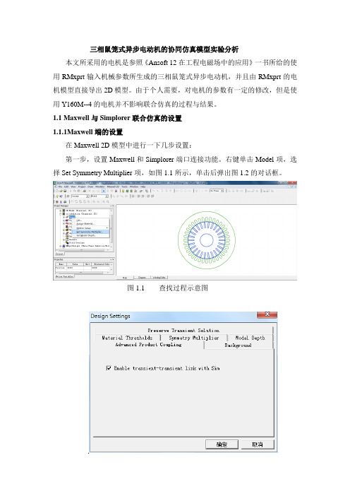
右键单击Model项,选择Set Symmetry Multiplier项,如图1.1所示,单击后弹出图1.2的对话框。
图1.1 查找过程示意图图1.2 设计设置对话框在对话框中,选择Advanced Product Coupling项,勾选其下的Enable tr-tr link with Sim 。
至此,完成第一步操作。
第二步,2D模型的激励源设置。
单击Excitation项的加号,显示Phase A、Phase B、Phase C各项。
双击Phase A项,弹出如图1.3所示的对话框。
图1.3 A相激励源设置在上图的对话框中,将激励源的Type项设置为External,并勾选其后的Strander,并且设置初始电流Initial Current项为0。
Number of parallel branch项按照电机的设置要求,其值为1。
参数设置完成后,点击确定退出。
需要说明的一点是,建议在设置Maxwell与Simplorer连接功能即第一步之前,记录电压激励源下的电阻和电感。
事实上,这里的电组和电感就是Maxwell 2D计算出的电机的定子电阻与定子电感。
这两个数据在外电路的连接中会使用到,在后面会详细说明。
至此,Maxwell端的设置完毕。
1.1.2 Simplorer端的设置Simplorer端的设置,主要是对电机外电路的设置,具体的电路会在空载实验和额定负载实验中详细给出,这里不再赘述。
Maxwell与Simplorer联合仿真方法及注意问题

三相鼠笼式异步电动机的协同仿真模型实验分析本文所采用的电机是参照《Ansoft 12在工程电磁场中的应用》一书所给的使用RMxprt输入机械参数所生成的三相鼠笼式异步电动机,并且由RMxprt的电机模型直接导出2D模型。
由于个人需要,对电机的参数有一定的修改,但是使用Y160M--4的电机并不影响联合仿真的过程与结果。
1.1 Maxwell与Simplorer联合仿真的设置1.1.1Maxwell端的设置在Maxwell 2D模型中进行一下几步设置:第一步,设置Maxwell和Simplorer端口连接功能。
右键单击Model项,选择Set Symmetry Multiplier项,如图1.1所示,单击后弹出图1.2的对话框。
图1.1 查找过程示意图图1.2 设计设置对话框在对话框中,选择Advanced Product Coupling项,勾选其下的Enable tr-tr link with Sim 。
至此,完成第一步操作。
第二步,2D模型的激励源设置。
单击Excitation项的加号,显示Phase A、Phase B、Phase C各项。
双击Phase A项,弹出如图1.3所示的对话框。
图1.3 A相激励源设置在上图的对话框中,将激励源的Type项设置为External,并勾选其后的Strander,并且设置初始电流Initial Current项为0。
Number of parallel branch项按照电机的设置要求,其值为1。
参数设置完成后,点击确定退出。
需要说明的一点是,建议在设置Maxwell与Simplorer连接功能即第一步之前,记录电压激励源下的电阻和电感。
事实上,这里的电组和电感就是Maxwell 2D计算出的电机的定子电阻与定子电感。
这两个数据在外电路的连接中会使用到,在后面会详细说明。
至此,Maxwell端的设置完毕。
1.1.2 Simplorer端的设置Simplorer端的设置,主要是对电机外电路的设置,具体的电路会在空载实验和额定负载实验中详细给出,这里不再赘述。
基于Simplorer与Maxwell的磁控电抗器特性仿真分析

comprehensive analysis of the response characteristic and magnetic field performance under the external complex
control circuit. In order to make up for this defect,
a new method for the field-circuit coupled multi-physics simulation
by combining Simplorer and Maxwell was introduced. By comparing and analyzing the relevant data of simulation with
Zhengzhou University,
Zhengzhou 450001,
Henan,
China;
2. Datang Central-China Electric Power Test Research
Institute,
Zhengzhou 450000,
Hee current simulation analysis method of magnetically controlled reactors cannot realize the
河南 郑州 450000)
摘要:磁控电抗器仿真分析方法无法实现在外部具有复杂控制电路下的响应特性与磁场性能的全面分
析。为了弥补这个缺陷,引入 Simplorer 与 Maxwell 联合实现场路耦合多物理域仿真的新方法,通过与 Matlab/
Simulink 仿真的相关数据对比,分析得出新的仿真分析方法更优,能为设计出性能更好的可控电抗器提供实
(完整版)Maxwell与Simplorer联合仿真方法及注意问题

三相鼠笼式异步电动机的协同仿真模型实验分析本文所采用的电机是参照《Ansoft 12在工程电磁场中的应用》一书所给的使用RMxprt输入机械参数所生成的三相鼠笼式异步电动机,并且由RMxprt的电机模型直接导出2D模型。
由于个人需要,对电机的参数有一定的修改,但是使用Y160M--4的电机并不影响联合仿真的过程与结果。
1.1 Maxwell与Simplorer联合仿真的设置1.1.1Maxwell端的设置在Maxwell 2D模型中进行一下几步设置:第一步,设置Maxwell和Simplorer端口连接功能。
右键单击Model项,选择Set Symmetry Multiplier项,如图1.1所示,单击后弹出图1.2的对话框。
图1.1 查找过程示意图图1.2 设计设置对话框在对话框中,选择Advanced Product Coupling项,勾选其下的Enable tr-tr link with Sim 。
至此,完成第一步操作。
第二步,2D模型的激励源设置。
单击Excitation项的加号,显示Phase A、Phase B、Phase C各项。
双击Phase A项,弹出如图1.3所示的对话框。
图1.3 A相激励源设置在上图的对话框中,将激励源的Type项设置为External,并勾选其后的Strander,并且设置初始电流Initial Current项为0。
Number of parallel branch项按照电机的设置要求,其值为1。
参数设置完成后,点击确定退出。
需要说明的一点是,建议在设置Maxwell与Simplorer连接功能即第一步之前,记录电压激励源下的电阻和电感。
事实上,这里的电组和电感就是Maxwell 2D计算出的电机的定子电阻与定子电感。
这两个数据在外电路的连接中会使用到,在后面会详细说明。
至此,Maxwell端的设置完毕。
1.1.2 Simplorer端的设置Simplorer端的设置,主要是对电机外电路的设置,具体的电路会在空载实验和额定负载实验中详细给出,这里不再赘述。
RMXPRT-MAXWELL和SIMPLORER的联合仿真解析
RMXPRT/MAXWELL和SIMPLORER的联合仿真解析
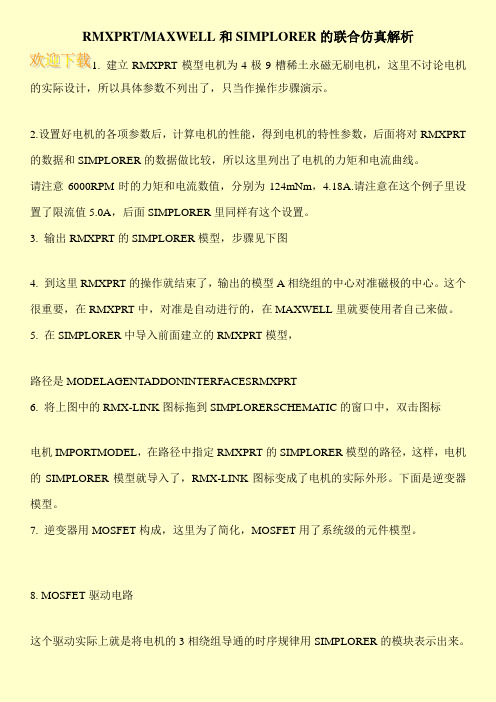
1. 建立RMXPRT模型电机为4极9槽稀土永磁无刷电机,这里不讨论电机的实际设计,所以具体参数不列出了,只当作操作步骤演示。
2.设置好电机的各项参数后,计算电机的性能,得到电机的特性参数,后面将对RMXPRT 的数据和SIMPLORER的数据做比较,所以这里列出了电机的力矩和电流曲线。
请注意6000RPM时的力矩和电流数值,分别为124mNm,4.18A.请注意在这个例子里设置了限流值5.0A,后面SIMPLORER里同样有这个设置。
3. 输出RMXPRT的SIMPLORER模型,步骤见下图
4. 到这里RMXPRT的操作就结束了,输出的模型A相绕组的中心对准磁极的中心。
这个很重要,在RMXPRT中,对准是自动进行的,在MAXWELL里就要使用者自己来做。
5. 在SIMPLORER中导入前面建立的RMXPRT模型,
路径是MODELAGENTADDONINTERFACESRMXPRT
6. 将上图中的RMX-LINK图标拖到SIMPLORERSCHEMATIC的窗口中,双击图标
电机IMPORTMODEL,在路径中指定RMXPRT的SIMPLORER模型的路径,这样,电机的SIMPLORER模型就导入了,RMX-LINK图标变成了电机的实际外形。
下面是逆变器模型。
7. 逆变器用MOSFET构成,这里为了简化,MOSFET用了系统级的元件模型。
8. MOSFET驱动电路
这个驱动实际上就是将电机的3相绕组导通的时序规律用SIMPLORER的模块表示出来。
Maxwell与Simplorer联合仿真
三相鼠笼式异步电动机的协同仿真模型实验分析本文所采用的电机是参照《Ansoft 12在工程电磁场中的应用》一书所给的使用RMxprt输入机械参数所生成的三相鼠笼式异步电动机,并且由RMxprt的电机模型直接导出2D模型。
由于个人需要,对电机的参数有一定的修改,但是使用Y160M--4的电机并不影响联合仿真的过程与结果。
1.1 Maxwell与Simplorer联合仿真的设置1.1.1Maxwell端的设置在Maxwell 2D模型中进行一下几步设置:第一步,设置Maxwell和Simplorer端口连接功能。
右键单击Model项,选择Set Symmetry Multiplier项,如图1.1所示,单击后弹出图1.2的对话框。
图1.1 查找过程示意图图1.2 设计设置对话框在对话框中,选择Advanced Product Coupling项,勾选其下的Enable tr-tr link with Sim 。
至此,完成第一步操作。
第二步,2D模型的激励源设置。
单击Excitation项的加号,显示Phase A、Phase B、Phase C各项。
双击Phase A项,弹出如图1.3所示的对话框。
图1.3 A相激励源设置在上图的对话框中,将激励源的Type项设置为External,并勾选其后的Strander,并且设置初始电流Initial Current项为0。
Number of parallel branch项按照电机的设置要求,其值为1。
参数设置完成后,点击确定退出。
需要说明的一点是,建议在设置Maxwell与Simplorer连接功能即第一步之前,记录电压激励源下的电阻和电感。
事实上,这里的电组和电感就是Maxwell 2D计算出的电机的定子电阻与定子电感。
这两个数据在外电路的连接中会使用到,在后面会详细说明。
至此,Maxwell端的设置完毕。
1.1.2 Simplorer端的设置Simplorer端的设置,主要是对电机外电路的设置,具体的电路会在空载实验和额定负载实验中详细给出,这里不再赘述。
基于Simplorer和Maxwell联合运行的线性压缩机仿真模拟

基于Simplorer和Maxwell联合运行的线性压缩机仿真模拟邹慧明;张立钦;彭国宏;田长青【摘要】基于Simplorer仿真软件和Maxwell磁场二维瞬态分析软件联合仿真平台,建立了线性压缩机的仿真模型,实现线性压缩机电磁场数值分析、机械振动动力学分析以及电路系统特性分析的联合仿真模拟.采用该仿真模型分析了线性压缩机在不同工况下的性能特点,并将仿真结果与样机压缩空气实验结果相比较,验证了仿真模型的可行性.【期刊名称】《压缩机技术》【年(卷),期】2011(000)001【总页数】6页(P7-11,14)【关键词】线性压缩机;仿真模拟;动力学【作者】邹慧明;张立钦;彭国宏;田长青【作者单位】中国科学院理化技术研究所,北京,100190;中国科学院理化技术研究所,北京,100190;中国科学院研究生院,北京,100190;中国科学院理化技术研究所,北京,100190;中国科学院理化技术研究所,北京,100190【正文语种】中文【中图分类】工业技术2011年第 1 期(总 225 期)文章编号:1006-2971f2011 ) 01-0007-06 0引言 Simplorer 和 Maxwell 联合运行的线性压缩机仿真模拟邹慧明1 ,张立钦1.2 .彭国宏1.2,田长青 1( 1.中国科学院理化技术研究所,北京 100190 ;2.中国科学院研究生院,北京 100190 )摘要:基于Simplorer‘仿真软件和Maxwell 磁场二维瞬态分析软件联合仿真平台,建立了线性压缩机的仿真模型,实现线性压缩机电磁场数值分析、机械振动动力学分析以及电路系统特性分析的联合仿真模拟。
采用该仿真模型分析了线性压缩机在不同工况下的性能特点,并将仿真结果与样机压缩空气实验结果相比较,验证了仿真模型的可行性。
关键词:线性压缩机;仿真模拟;动力学中图分类号: TH457文献标志码:A Simulationof LinearCompressorBasedonSimplorerandMaxwell ZOUHui-ming',ZHANGLi-qin"2.PENG Guo-hong"2,TIAN hang-qingl ( 1.Technical InstituteofPhysics andChem 厶try,ChineseAcademyofScien.ces,Beijing100190,Chinn.; 2.GraduateUniversity ofChinese AcademyofSciences,Beijing100190,China)Abstract:Thispaperestablishes asimulationmodelfor linear compressorbasedonSimplorersimulationplat-formandMaxwellsimulation platform to achieve the jointsimulation ofelectromagneticfield,mechanicaldynam-ics andelectricalsystemanalysis onlinear compressor.Thecharacteristicsof linear compressorworkingwiLh airon variable conditionsareanalyzedby the simulationmodel.Thesimulation modelis validated well by the com- parisonbetweenthe simulationresultsandthe experimentaldata. Keywords:linearcompressor;simulation ;dynamics采用直线振荡电机作为驱动装置的线性压缩机主要由机械系统(直线电机驱动活塞往复运行)、电磁系统(电源驱动直线电机)和热力系统(活塞压缩气缸内气体)组成,相比于传统旋转电机驱动的活塞压缩机,该类压缩机效率较高。
基于Simplorer与Maxwell的磁控电抗器特性仿真分析

基于Simplorer与Maxwell的磁控电抗器特性仿真分析赵国生; 孙彬; 李培; 原峰【期刊名称】《《电气传动》》【年(卷),期】2019(049)010【总页数】5页(P91-95)【关键词】磁控电抗器; 双级磁阀; 谐波; 响应【作者】赵国生; 孙彬; 李培; 原峰【作者单位】郑州大学电气工程学院河南郑州 450001; 大唐华中电力试验研究院河南郑州 450000【正文语种】中文【中图分类】TM28磁控电抗器(magnetically controlled reactors,MCR)作为一种新型无功补偿装置,优化分析其谐波、响应特性等对于改善供电质量、提高电网经济效益起着重要的作用。
目前,对于可控电抗器特性分析方法主要有理论分析方法[1]、Matlab/Simulink仿真分析法和Ansoft Maxwell仿真分析法。
理论分析方法从计算公式推导上详细介绍了新型可控电抗器的工作原理及特性分析等,其缺点是不能直观地反映谐波、磁场和响应等特性的变化过程。
Matlab/Simulink仿真分析法虽然可以搭建仿真电路,但仅能用变压器等效饱和式电抗器模型,且与文中饱和式可控电抗器的仿真模型类似,该方法对单相可控电抗器[2-4]、单相三柱式MCR[5-6]、单相四柱式 MCR[7-11]及三相三柱式MCR[12]等的谐波及响应特性进行了分析,该方法缺陷是不能对硅钢片参数进行精确的磁化曲线拟合,尤其是无法构造特殊磁阀模型,如单级、双级以及多级模型,也无法分析模型的磁场变化。
Ansoft Maxwell仿真分析法对单相四柱式MCR[13]、三相六柱式 MCR[14]和正交铁心三相磁控电抗器[15]等进行了电磁仿真及谐波特性分析,虽然该方法弥补了Matlab/Simulink仿真分析法的部分不足之处,但又因其电路简单而无法实现复杂控制电路的响应特性分析。
为了实现波形及磁场变化的观察分析,并且解决硅钢片B—H拟合曲线、特殊磁阀构造及复杂电路搭建等问题,本文引入了Simplorer与Maxwell联合仿真的方法[16-17],Simplorer是功能强大的多域机电系统设计与仿真分析软件,用于电磁、控制等机电一体化系统的建模、设计、仿真分析和优化,与Maxwell联合实现场路耦合多物理域联合仿真,将大大提高仿真特性的真实性和准确性。
- 1、下载文档前请自行甄别文档内容的完整性,平台不提供额外的编辑、内容补充、找答案等附加服务。
- 2、"仅部分预览"的文档,不可在线预览部分如存在完整性等问题,可反馈申请退款(可完整预览的文档不适用该条件!)。
- 3、如文档侵犯您的权益,请联系客服反馈,我们会尽快为您处理(人工客服工作时间:9:00-18:30)。
T1T2T3T4Co-simulation with Maxwell Technical BackgroundThe co-simulation is the most accurate way of coupling the drive and the motormodel. The advantage of this method is the high accuraty, having the realinverter currents as source in Maxwell and the back emf of the motor on theinverter currents as source in Maxwell, and the back-emf of the motor on theinverter side.The transient-transient link enables the use to pass data between Simplorer andMaxwell during the simulation:Maxwell2D and Maxwell3D can be usedSimplorer and Maxwell will run altogetherSimplorer is the Master, Maxwell is the slaveAt a given time step, the Winding currents and the Rotor angle are passedfrom Simplorer to Maxwell, the Back EMF and the Torque are passed fromMaxwell to SimplorerThe complexity of the drive system and of the mechanical system is notThe complexity of the drive system and of the mechanical system is notlimitedInsights on the coupling MethodThe Simplorer time steps and the Maxwell time steps don’t have to be thesame. Usually, Simplorer requires much more time steps than Maxwell.Assume the current simulation time is tSimplorer, based on the previous time steps, gives a forward meeting timet1to Maxwell where both simulators will exchange data. Between t0and t1,both code run by themselves.At t1, both codes exchange data. If during the t0-t1period, some eventappears on Simplorer side (state graph transition, large change of thepp p(g p,g gdynamic of the circuit), Simplorer will roll back to t0and set a new forward meeting time t1’, t1’< t1.the Basic Elements > Circuit > Semiconductors System Level libraryCo-simulation with Maxwell Simplorer SchematicWe use a control signal for each igbt. IGBT1has the igbt1control signal (youneed to uncheck the use Pin button). Name the control signals of IGBT2toIGBT6 accordingly.Follow the naming as belowCo-simulation with Maxwell Simplorer SchematicThe reference waveforms are implemented using time functions: pick the SineWave in the Basic Elements > Tools > Time Functions library.Put 3 Sine Wave blocks on the schematic, with the parameters as aboveAdd a Triangular wave time function blockThe switching of the IGBTs is done through a state graph that will compare thereference wave forms and the chopper signalCo-simulation with Maxwell Simplorer SchematicSimplorer SchematicIn the Basic Elements > States library, pick up two STATE_11, two TRANSBuild the graph below then make two additional copies to have 3 circuits, one foreach phaseFor the first state graph, we will monitor IGBT1and IGBT2Co-simulation with Maxwell Maxwell in SimplorerIn order to use a Maxwell model in co-simulation with Simplorer, the user justneeds to do a couple of modifications on the Maxwell side.Right mouse click on the Maxwelldesign name and select copyRight mouse click on the Project name and select pasteRename the copied design name in 2_Maxwell_SimplorerCo-simulation with Maxwell Maxwell in SimplorerRight mouse click on Model, and select Symmetry MultiplierGo to the Advanced Product Coupling tab and enable transient-transient link withSimplorer. That will let Maxwell know that everything linked to rotor position and winding information are to be taken from SimplorerGo to the winding definition under the Excitation tab, Right mouse click onPhaseA, then select PropertiesCo-simulation with Maxwell Maxwell in SimplorerFor each winding, you need to enter that you want the current information to beread in Simplorer.Select External in the ‘Type’ pull down menuMake sure that the initial current is 0Make sure that the initial current is0Repeat the same operation for PhaseB and PhaseC.That’s all for the Maxwell part.Save and close the Maxwell project.Make sure to know where the project is saved on the diskMake sure to know where the project is saved on the diskCo-simulation with Maxwell Simplorer SchematicGo to Simplorer Circuit > Subcircuit > Maxwell Component > Add TransientCosimulationIn the Transient-Transient coupling window, open the link File aera, and selectthe Maxwell projectCo-simulation with Maxwell Simplorer SchematicMaxwell is opened and loads the projectOn the Transient-Transient link Simplorer window, the project information areloadedSelect 2D for the Design type, and choose the design 2_Maxwell_SimplorerIn the Options tab, select Pin Description and click OK.Co-simulation with Maxwell Simplorer SchematicPlace the Component on the schematic, nearby the phase resistancesThe component has 8 pins : 2 pins for each phase and 2 mechanical pins for therotorWe need to increase the symbol size. In the Definitions> Components tab of theSimplorer project window, rigth mouse click on MxTranTranData2 (thecomponent name) and select Edit SymbolCo-simulation with MaxwellSimplorer SchematicThe Symbol Editor window pops upClick on the motor image, and move the image away in order to have access to g g ythe symbol footprintCo-simulation with Maxwell Simplorer SchematicEnlarge the footprint to the desired size.The Pins should also be moved, as well as the pin description text zonesThe motor image needs to be resized and re centeredThe motor image needs to be resized and re centeredCo-simulation with Maxwell Simplorer SchematicUpdate the project, using the icon,just above the project nameOnce the project is updated, double click on the schematic name, then wire themotor to the phase resistances. PhaseA_out, PhaseB_out and PhaseC_outpinsare linked together in this exampleCo-simulation with Maxwell Simplorer SchematicA constant speed is used. Go to the Component tab, in the Basic Elements >Physical Domains > Mechanical > Velocity –Force –Representation >Rotational_V folder, choose the V_ROT: Angular Velocity SourceRotational V folder choose the V ROT:Angular Velocity SourceEnter 4500rpm and link this component to the MotionSetup1_out pinLink the MotionSetup1pin to the (mechanical) groundNote: Simplorer allows you to have much more complicated mechanical systemsCo-simulation with Maxwell Simplorer SimulationBefore simulating, the outputs data that will be available in Simplorer need to bedefined. Open the Output DialogBy default, most of the common outps are saved by default. Browse to the FEA1folder, then select the desired outps from Maxwell2D that you want to keep, then click on OK。