UG-cae结构分析
基于UGCAE的平面六杆机构的运动分析

基于UG/CAE的平面六杆机构的运动分析1、题目说明如上图所示平面六杆机构,试用计算机完成其运动分析。
已知其尺寸参数如下表所示:题目要求:两人一组计算出原动件从0到360时(计算点数37)所要求的各运动变量的大小,并绘出运动曲线图及轨迹曲线。
注:为了使计算的结果更好的拟合运动的实际情况,同时考虑到UG在运动仿真分析计算方面的快速性,我们决定在绘制曲线时将计算点由37点增加到600点。
数据输出到Excel表格时计算点取100点。
建模及其分析方法附后!2、建模及其运动分析软件介绍:UG NX是集CAD\CAE\CAM于一体的三维参数化软件,也是当今世界最先进的设计软件,它广泛应用于航空航天、汽车制造、机械电子等工程领域。
还有在系统创新、工业设计造型、无约束设计、装配设计、钣金设计、工程图设计等方面的功能。
运动仿真是UG/CAE(Computer Aided Engineering)模块中的主要部分,它能对任何二维或三维机构进行复杂的运动学分析、动力分析和设计仿真。
通过UG/Modeling的功能建立一个三维实体模型,利用UG/Motion的功能给三维实体模型的各个部件赋予一定的运动学特性,再在各个部件之间设立一定的连接关系既可建立一个运动仿真模型。
UG/Motion的功能可以对运动机构进行大量的装配分析工作、运动合理性分析工作,诸如干涉检查、轨迹包络等,得到大量运动机构的运动参数。
通过对这个运动仿真模型进行运动学或动力学运动分析就可以验证该运动机构设计的合理性,并且可以利用图形输出各个部件的位移、坐标、加速度、速度和力的变化情况,对运动机构进行优化。
我们通过学习UG,通过建立平面六杆机构模型,通过UG/CAE模块对平面连杆的运动进行分析。
3.六连杆机构的三维造型连杆L1连杆L2连杆L3连杆L5连杆L6六杆机构装配示意图机构装配后运动演示见附件—平面六杆运动演示.avi (本报告相同目录下)3. 运动分析数据计算结果在附件的Excel表格中。
UG运动仿真分析

· 固定副 在连杆间创建一个固定连接副,相当于以刚性连接两连杆,连杆间无相 对运动。
特殊运动副:
· 齿轮齿条副:滑动副和旋转副的结合 · 齿轮副:两个转动副的结合 · 线缆副:两个滑动副的结合 · 点线接触副:4个自由度 · 线线接触副: 4个自由度 · 点面副:5个自由度
UG提供了12种运动副共分两大类:普通运动副 8种,它是独特的,于自身有关;特殊运动副4种, 是在两个普通类型的运动副之间定义了特殊关系的 运动副,允许两个不同类型的运动副一起工作完成 特定的功能。
普通运动副
· 旋转副
连接两个连杆的经典运 动副,有 一个绕Z轴旋 转的自由度,不允 许两个连杆之间有任何的移动。
· 球铰
关节运动仿真,通过控制一个或多个原动运动副的位移步 长来进行机构动态仿真。位移为步长大小和步数的乘积。
· 生成图表
动画或关节仿真后,可通过图表方式输出机构的分析结果。 Y-轴:可通过下拉菜单设置Y轴参数。 值:‘幅值’和‘角度幅值’表示参数是各分量的合成量, T1,T2,T3和输入角度1、2、3分别表示所选参数的沿坐 标轴的三个水平分量或转动分量。
· 运动副
以一定的方式把各个构件彼此非刚性(可动)联接, 构件间能产生某些相对运动。
· 自由度和约束
任意两个没有构成运动副的构件,两者之间有6个 自由度(在坐标系中3个运动和3个转动)。若将两 者以某种方式联接而构成运动副,则两者的相对运 动便受到一定的约束。
2. Scenario 模型
选 择 [ 应 用 ] - [ 运 动 ] 命令,进入运动分析模块。单击 右侧“Scenario 导航器”,弹出下图。
基于UG的注塑模具研究

基于UG的注塑模具研究一、本文概述随着现代制造业的快速发展,注塑模具作为塑料制品生产中的重要工艺装备,其设计、制造和应用水平直接影响到产品的质量和生产效率。
因此,对注塑模具的研究与改进一直是制造业领域的热点课题。
本文旨在探讨基于UG(Unigraphics N,一款广泛应用的CAD/CAM/CAE 集成软件)的注塑模具研究,通过对UG软件在注塑模具设计、分析、优化等方面的应用进行深入分析,以期提高注塑模具的设计效率、制造精度和使用性能。
本文将首先介绍注塑模具的基本原理和分类,阐述注塑模具在现代制造业中的重要地位和作用。
接着,重点分析UG软件在注塑模具设计中的应用,包括模具型腔设计、浇注系统设计、冷却系统设计等方面。
还将探讨UG软件在注塑模具分析和优化方面的功能,如模具流场分析、结构强度分析、热平衡分析等。
通过实际案例的分析和比较,展示UG软件在注塑模具研究中的实际应用效果,为相关领域的研究人员和工程师提供有益的参考和借鉴。
通过本文的研究,旨在推动基于UG的注塑模具设计的理论创新和技术进步,为提升我国制造业的整体竞争力和可持续发展贡献力量。
二、注塑模具基础知识注塑模具,亦称为塑料注射模具,是塑料加工工业中广泛使用的一种成型工具。
它的主要工作原理是,通过注塑机将熔融的塑料注入模具型腔,经冷却固化后,获得所需形状和尺寸的塑料制品。
注塑模具的设计、制造质量直接影响到产品的质量和生产效率,因此,对注塑模具的研究具有重要意义。
注塑模具通常由动模、定模两大部分组成,动模和定模在注塑机的合模机构作用下闭合,形成模具型腔。
模具型腔的形状和尺寸决定了塑料制品的外形和尺寸。
另外,注塑模具还包括浇注系统、导向机构、脱模机构、侧向分型与抽芯机构、温度调节系统等组成部分,这些部分共同保证了注塑过程的顺利进行。
在注塑模具的设计过程中,需要考虑的因素包括塑料的性能、产品的结构、注塑机的类型及规格、模具的制造工艺等。
设计合理的浇注系统可以保证塑料在模具型腔中均匀流动,避免产生气泡、缩孔等缺陷。
NX CAE跌落分析实例详解
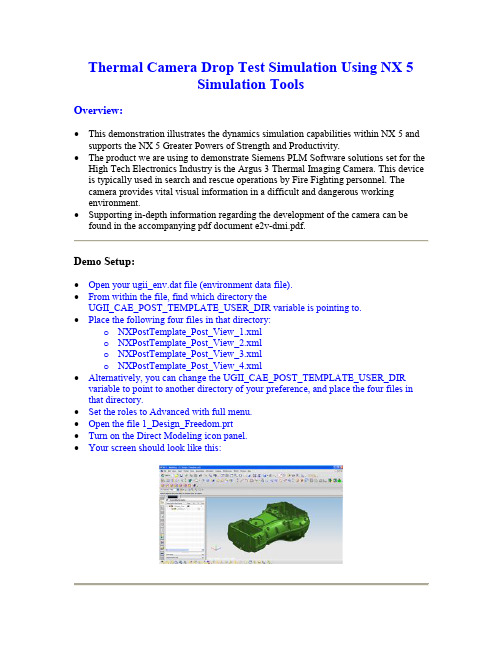
Thermal Camera Drop Test Simulation Using NX 5Simulation ToolsOverview:∙This demonstration illustrates the dynamics simulation capabilities within NX 5 and supports the NX 5 Greater Powers of Strength and Productivity.∙The product we are using to demonstrate Siemens PLM Software solutions set for the High Tech Electronics Industry is the Argus 3 Thermal Imaging Camera. This device is typically used in search and rescue operations by Fire Fighting personnel. The camera provides vital visual information in a difficult and dangerous workingenvironment.∙Supporting in-depth information regarding the development of the camera can be found in the accompanying pdf document e2v-dmi.pdf.Demo Setup:∙Open your ugii_env.dat file (environment data file).∙From within the file, find which directory theUGII_CAE_POST_TEMPLATE_USER_DIR variable is pointing to.∙Place the following four files in that directory:o NXPostTemplate_Post_View_1.xmlo NXPostTemplate_Post_View_2.xmlo NXPostTemplate_Post_View_3.xmlo NXPostTemplate_Post_View_4.xml∙Alternatively, you can change the UGII_CAE_POST_TEMPLATE_USER_DIR variable to point to another directory of your preference, and place the four files in that directory.∙Set the roles to Advanced with full menu.∙Open the file 1_Design_Freedom.prt∙Turn on the Direct Modeling icon panel.∙Your screen should look like this:∙Rotate and zoom the part as appropriate to give the audience a feel for the part. ∙From Direct Modeling, select Delete Face.∙Change the type to Hole.∙Make sure Select Holes by Size is not checked as an option.∙Zoom in on the part and select the following hole:∙Click Apply.∙After the hole is deleted, your part should look like this:∙From the Delete Face form, change the type from Hole to Face.∙Change the Filter Face Rule to Slot Faces.∙From the same graphical view, select the following face (the entire slot will chain from one selection):∙Click Apply.∙The slot will disappear.∙Rotate the part over 180º about the z axis.∙Your view should look like this:∙Zoom in if needed.∙Change the Filter Face Rule to Region Faces.∙First select a Seed Face. Pick one of the surfaces inside the channel.∙Next select all the bounding surfaces of the channel.∙Click MMB.∙Click OK.∙Note: You will have selected a total of 8 faces. One for the seed face, and seven for the boundary region faces.∙This concludes the Design Freedom portion of the demo.∙From the menu, select File, Close, All Parts.∙Click Yes when prompted (do not save your work).∙Open the file 2_Pre_Processing.sim.∙You may need to set the filter to Simulation Files (*.sim).∙Rotate the part and zoom-in as appropriate, to give the audience a feel for the mesh.∙When finished, make sure the display screen on the thermal camera is facing up (as shown below).∙Click on 2D Collectors to expand the list. Turn off the display for the collector Outer_Shell_Suppress.∙Rotate the part and zoom-in as appropriate, to give the audience a feel for the mesh.∙Your display should now look like:Click on 3D Collectors to expand the list. Turn off the display of viewscreen, view face plate, and battery cover.∙Rotate the part and zoom-in as appropriate, to give the audience a feel for the mesh.∙Your display should now look like:∙Under 2D Collectors, turn off the display of the collector Outer Shell.∙Rotate the part and zoom-in as appropriate, to give the audience a feel for the mesh.∙Your display should now look like:∙Again in 2D Collectors, turn off the display of Interface PCB.∙In 1D Collectors, turn off the display of RBE3 (You will need to expand the 1D Collectors list).∙Rotate the part and zoom-in as appropriate, to give the audience a feel for the mesh.∙Your display should now look like:∙From the Simulation Navigator, turn off the display of all 1D Collectors.∙Rotate and zoom-in on the part as appropriate.∙Your display should now look like this:∙Turn off the display of all remaining finite elements by clicking on 2D Collectors and 3D Collectors.∙Turn on all of the geometry by clicking on Polygon Geometry.∙Your display should look like this:∙Rotate the part and zoom-in as appropriate, to give the audience a feel for the model.∙From the menu, click on Format, Visible in View.∙Click OK on the Visible Layers in View form.∙Next click on Outer_Shell, Invisible, Apply. Rotate / zoom-in on the part as needed.∙Repeat the previous step for Battery and View_Screen.∙Repeat the previous step for Internals, but instead of clicking Apply, click on OK.∙Your display should now look like the following:After removing Outer_ShellAfter removing BatteryAfter removing View_ScreenAfter removing InternalsIn Simulation Navigator, click on the sim file to highlight it (2_Pre_Processing).Next RMB and select New Solution.connecting parts. But first we must create a solution to contain all of the simulation related data.∙Give the solution a name, such as Resp_Sim_Modal.∙Change the Solution Type to SEMODES 103 – Response Simulation.First window that pops upWindow changes when you change the Solution Type ∙Click OK.∙Click on the Surface-to-Surface Gluing icon.∙From the pop-up window, change the search distance to 0.1 mm. ∙Click on Create Face Pairs.∙From the next window, change the Grouping Option to One. ∙Change the Distance Tolerance to 0.1 mm.∙Click on Preview.∙The window should indicate 24 face pairs found. ∙Click OK on three windows.Your display should now look like this:∙From the Simulation Navigator, located under the Simulation Object Container, there will be a node for Face Gluing(1).∙You may need to expand the Simulation Object Container to find it.∙Place the cursor over the Face Gluing(1) node until the glue definitions in the display window are highlighted.∙Click RMB Edit. A window will pop up.∙Click on each of the Source Region and Target Region areas in the pop-up window to show that they are highlighted in the display window.∙Click Cancel.∙From the Simulation Navigator, turn off the display of the Polygon Geometry and the Face Gluing(1) object (located in Simulation Object Container).∙Your screen will now be blank.∙Turn on the display of all 1D Collectors, 2D Collectors, and 3D Collectors.∙Your screen will now look like:∙From the Simulation Navigator, RMB click on Constraints.∙Select New Constraint, Enforced Motion Location.∙Select the independent node at the center of the RBE2 (RBE2_spider_mesh(3). ∙The node label is 106991.∙Make DOF1, DOF2, and DOF3 Enforced. Make DOF4, DOF5, and DOF6 Free. ∙Click OK.∙From the Simulation Navigator, RMB click on Subcase – Dynamics, then select Edit Attributes.∙Next click on Create Modeling Object (Next to Output Requests).∙Give the Object a name (something such as My Output).∙Click on a few of the tabs to show the different outputs available (i.e. Strain, Acceleration, Displacement, etc.).∙Make sure that as a minimum, Strain and Displacement are turned on for output. ∙Explain that these outputs are needed later for the Response Simulation Analysis. ∙Scroll down to the bottom of this window.∙Show how the user can select to have the output generated for the whole model (default is All) or they can switch to Set and pick an element set or node set,depending on the output type.∙Click on Preview.∙An information window will pop up, showing the outputs that are selected for analysis.∙Close the information window.∙Click OK on the Output Requests form.∙Next click on Create Modeling Object (Next to Lanczos Method).∙Give the Object a name (such as All Modes < 300 Hz).∙Enter 300 in the box next to Frequency Range – Upper Limit.∙Click OK twice.∙Explain that the next step would be to click RMB Solve on the Resp_Sim_Modal that was created. This would solve the job, but this will take too much time for a live demo. The solution is already completed, and you will skip over by loading the next part.∙From the menu, select File, Close, All Parts.∙Do not save the work that was done.∙Click on Yes when it prompts if you want to close.∙Open the sim file 3_Post.sim.∙Click on Post-Processing Navigator.∙Double click the Resp_Sim_Modal tab. This will load the modal results.∙Click on the + Resp_Sim_Modal tab to expand the list of results.∙Click on the + Mode 12 tab to expand the list.∙Double click on the Displacement – Nodal to plot the results for Mode 12.∙Your screen should now look like this:∙Double click on the post-processing template Post_View_1.∙It is located down near the bottom of the Post-Processing Navigator window. ∙Your screen should now look like this:∙Turn on the Post Processing icon panel.∙Click on Animation.∙Change Style to Modal.∙Click on the Full Cycle box.∙Click OK.∙Your screen should now look like this:∙Rotate and zoom in on the part as appropriate.∙When done viewing the animation, click Stop.∙Show any of the other modes, as time and interest permit. To show another mode, expand its results and double click on the Displacement – Nodal tab for that result.Press Play for the animation to resume.∙When done showing modal results animations, click on the Stop icon.∙Scroll up and down the list of modal results (in the Post-Processing Navigator).∙Show the audience that the first three results are the rigid body modes for the three DOF that were left free. The last three modes are constraint modes for thethree DOF that were specified as enforced.∙Go back into Simulation Navigator.∙Turn on the Response Simulation toolbar.∙Click on the Create Response Simulation icon.∙Give the Simulation a name, such as Drop Test.∙Make sure the Resp_Sim_Modal results are selected on the form.∙Set the Rigid Body Mode Frequency Tolerance to 1.∙Any mode below 1 Hz is assumed to be a rigid body mode, and is ignored. ∙Click OK.∙On the simulation you just created (Drop Test), click RMB Create Event. ∙Give the event a name, such as Y_Impact.∙Set the type to Transient.∙Set the Data Recovery Method to Mode Displacement.∙Set the duration to 0.01.∙The Initial Conditions should be Zero.∙Click OK.∙Click on XY Function Navigator.∙RMB click on Associated AFU and select Open.∙From the pop-up window, select the file 3_Post_Input_Excitation.afu ∙Click OK.∙Click on the afu you just imported to expand the list. ∙Double click on the height6ft-concrete1 function.∙It is the only function in the afu file.∙The function is plotted in the viewport.∙Click on Simulation Navigator.∙Turn on the Layout Manager toolbox. ∙Click on the Return to Model icon.∙RMB click on the Excitations tab under the event you created earlier (Y_Impact). ∙Select New Excitation, Create Translational Nodal Excitation.∙Select Enforced Motion from the Excitation option.∙Next to ID, select Excitation Location List.∙There should only be one option to pick from the pop-up window (Node 106991). ∙Select it.∙Click OK.∙Zoom in on the node that has the enforced DOF defined in the modal analysis.∙This is to remind the audience where this originated from.∙Under Excitation Functions, turn off X and Z options.∙Click on the arrow next to the Y option. Select Function Manager.∙Select the function height6ft-concrete1.∙This is the only selection you can make.∙Click OK.∙Give the excitation a name, such as Concrete 6ft drop.∙Click OK.∙Expand the Response Simulation Details View.∙Click on Normal Modes [30], located under Drop Test, to highlight it.∙Show how the damping is currently set to zero.∙RMB click on the Normal Modes (located under Drop Test in the Navigator pane) and select Edit Damping Factor.∙For damping, enter 20% Viscous damping.∙Click OK.Show how the damping factors (viscous) have been updated.∙Collapse the Response Simulation Details View.∙RMB click on the event you created (Y_Impact) and select Solve for ModalResponse. (The solution should not take more than a few seconds).∙From Response Simulation, click on Evaluate Response Results.∙Make sure only Displacement is turned on in the form.∙For Select Nodes, pick Select All.∙The icon is located in the Selection Bar toolbox, you may have to add this icon from Customize.∙Set the Decimation Order to 10.∙Click OK.∙The solution should take approximately 1 minute.∙Anything significantly longer than this would indicate a problem.∙The progress bar should move steadily the whole time.∙Click on Post-Processing Navigator.∙Under Drop Test, RMB Select Y_Impact and click on Load.∙This will load the results.∙Expand the Y_Impact results.∙Expand the results for Increment 1.∙Double click on the Displacement – Nodal results for this increment. ∙Right click on the Post_View_2 line under Templates.∙Click Apply.∙Your screen should now look like this:∙Click on Animation.∙Change the Animate options to Iterations.∙Make sure the Step option is set to 1.∙Click on Play.∙Click OK.∙Your screen should now look like this:∙Rotate and zoom the part to give the audience different perspective views of the animation.∙Click on Stop.∙Double click on the template Post_View_3.∙Click Play.∙Your screen should now look like this:∙Click Stop.∙From Layout Manager, click on Return to Model.∙Click on Simulation Navigator.∙Turn off the display of all finite element entities (all collectors, simulation object containers, load and constraint containers, simulation objects, constraints, etc.) and all polygon geometry. Your screen should now be blank.∙Under 2D Collectors, turn on the display of U-Imaging Processor PCB.∙Click on Polygon Geometry to expand the list.∙Scroll down towards the bottom. There are three items named PLC44. Turn all three of them on.∙Earlier in the list there is a group of bodies you need to turn on. The first is SO6OPTO. Turn on this body.∙Going up in the list, skip the next 4 entities (all named CRSMD8), and turn on DIOD47 up through Polygon Body_92 (nine entities total).∙You will have turned on 13 total items.∙Your display should now look like this:∙Click RMB on the Y_Impact event.∙Select Evaluate Function Response, Elemental Function.∙Change the result type to Strain.∙Change the data component to Vonmises.∙Turn on the Store to AFU option.∙Turn off the XY Graphing option. (This is done to show that the results are stored as afu data and can be plotted individually. Alternatively, you can keep the XY Graphing option on and they will be plotted automatically. But be sure to go back and show the afu functions in navigator, and how the user can plot differentcombinations of the curves.)∙Give a prefix name such as PCB_Strain.∙Pick a series of elements from the viewport such as follows:∙Selections are shown in orange.∙ A number around 20 will be reasonable.∙Click OK.∙The solution should only take approximately 20 seconds.∙From the Navigator window, select the data you generated. ∙Click RMB Plot(XY).∙Click on Probing Mode.∙From the XY Plot, find the peak with your cursor and click LMB. ∙Identify the element label that corresponds to the peak curve.1.Match the line (color and dash style) with the legend.2.The legend text contains the element number.∙From Layout Manager, pick Return to Model.∙Click on Evaluate Response Results.∙Turn on Strain.∙Change the filter method to Related Elements.∙Pick one of the elements from the PCB.∙This filter selection should include 1756 elements.∙Change the Method to From XY Graph.∙Click on Select graph points.∙From the Equation Selection window, pick the function corresponding with the element having peak strain from the previous graph.∙Click OK.∙From the graph that appears, find the peak strain and click on it (LMB).∙Click MMB. (Or click on the green check mark).∙The next form will pre-populate with the corresponding time at which that strain occurs.∙Explain you would normally Click OK on the Evaluate Response Results form. ∙But the solution takes too long for a live demo.∙Click Cancel.∙Click File, Close, All Parts.∙Click Yes when prompted.∙Open the sim file 4_Post_Part2.sim.∙Click on Post-Processing Navigator.∙On the Y_Impact event, click RMB Load.∙This will load the results.∙Click on the + Y_Impact event to expand the results.∙Click on Response Results 2 to expand the list.∙Expand the list for Strain – Element-Nodal.∙Double click on the Von-Mises component to display the strain results.∙Double click on the post-processing template Post_View_4.∙Rotate and zoom the model as appropriate.∙The demo is complete.∙Do not save any work when exiting or closing files.∙During the course of the demo, three files will be created that you should delete prior to performing another demo.∙These files may possibly cause conflict for subsequent demos.1.3_post-drop_test-y_impact.afu2.3_post-drop_test-y_impact.rs23.3_post-drop_test-y_impact.eef。
UG软件的高级仿真教程
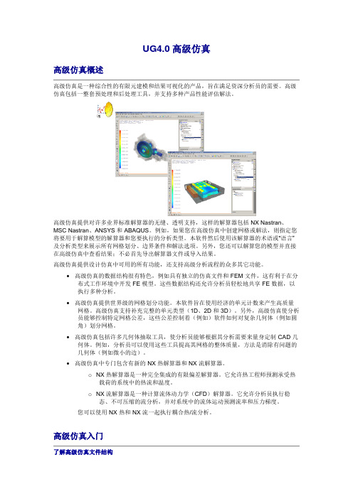
UG4.0高级仿真高级仿真概述高级仿真是一种综合性的有限元建模和结果可视化的产品,旨在满足资深分析员的需要。
高级仿真包括一整套预处理和后处理工具,并支持多种产品性能评估解法。
高级仿真提供对许多业界标准解算器的无缝、透明支持,这样的解算器包括 NX Nastran、MSC Nastran、ANSYS 和 ABAQUS。
例如,如果您在高级仿真中创建网格或解法,则指定您将要用于解算模型的解算器和您要执行的分析类型。
本软件然后使用该解算器的术语或“语言”及分析类型来展示所有网格划分、边界条件和解法选项。
另外,您还可以解算您的模型并直接在高级仿真中查看结果;不必首先导出解算器文件或导入结果。
高级仿真提供设计仿真中可用的所有功能,还支持高级分析流程的众多其它功能。
•高级仿真的数据结构很有特色,例如具有独立的仿真文件和 FEM 文件,这有利于在分布式工作环境中开发 FE 模型。
这些数据结构还允许分析员轻松地共享 FE 数据,以执行多种分析。
•高级仿真提供世界级的网格划分功能。
本软件旨在使用经济的单元计数来产生高质量网格。
高级仿真支持补充完整的单元类型(1D、2D 和 3D)。
另外,高级仿真使分析员能够控制特定网格公差,这些公差控制着(例如)软件如何对复杂几何体(例如圆角)划分网格。
•高级仿真包括许多几何体抽取工具,使分析员能够根据其分析需要来量身定制 CAD 几何体。
例如,分析员可以使用这些工具提高其网格的整体质量,方法是消除有问题的几何体(例如微小的边)。
•高级仿真中专门包含有新的 NX 热解算器和 NX 流解算器。
o NX 热解算器是一种完全集成的有限偏差解算器。
它允许热工程师预测承受热载荷的系统中的热流和温度。
o NX 流解算器是一种计算流体动力学(CFD)解算器。
它允许分析员执行稳态、不可压缩的流分析,并对系统中的流体运动预测流率和压力梯度。
您可以使用 NX 热和 NX 流一起执行耦合热/流分析。
高级仿真入门了解高级仿真文件结构高级仿真在四个独立而关联的文件中管理仿真数据。
ug建模介绍PPT课件

参数化设计
参数化设计能够大大提高设计的 灵活性和可维护性,未来UG建 模将进一步完善参数化设计功能, 方便用户进行定制化设计和修改。
多领域协同
未来UG建模将进一步支持多领 域协同设计,实现不同领域之间 的数据共享和交互,提高设计效
率和质量。
技术发展趋势
云技术应用
随着云技术的发展,UG建模将进 一步实现云端化,用户可以在云 端进行建模、渲染、仿真等操作,
03
UG建模实例教程
实例一:简单零件建模
总结词:基础入门
详细描述:本实例将介绍如何使用UG软件进行简单的零件建模,包括基本操作 、草图绘制、特征创建等,适合初学者入门学习。
实例二:复杂零件建模
总结词:进阶提高
详细描述:本实例将介绍如何使用UG软件进行复杂零件建模,涉及更高级的草图绘制、特征创建和编辑技巧,适合有一定基 础的学员进阶提高。
实例三:装配体建模
总结词:综合应用
详细描述:本实例将介绍如何使用UG软件进行装配体建模,包括零件的导入、装配约束的设置、装配 体的运动模拟等,适合学员全面掌握UG建模技术。
04
UG建模常见问题及解决方案
问题一:如何提高建模效率?
总结词:掌握UG软件常用命令和工具, 熟悉建模流程,提高建模效率。
航空航天领域
UG建模将进一步拓展到航空航天领域,涉及飞机设计、火箭设计、 卫星设计等高精度、高安全性的设计领域。
模具制造领域
UG建模在模具制造领域的应用将进一步深化,涉及模具结构设计、 仿真分析、加工制造等全流程的设计和管理。
感谢您的观看
THANKS
UG建模介绍PPT课件
目录
• UG建模软件概述 • UG建模基本操作 • UG建模实例教程 • UG建模常见问题及解决方案 • UG建模未来发展与展望
基于UG的数控编程及加工自动化的研究
基于UG的数控编程及加工自动化的研究一、本文概述随着现代制造业的快速发展,数控编程及加工自动化已成为提高生产效率、降低生产成本、保证产品质量的重要手段。
UG(Unigraphics N)作为一款功能强大的三维CAD/CAM/CAE集成软件,广泛应用于航空、汽车、模具等制造领域,其数控编程及加工自动化功能更是受到了广大制造业企业的青睐。
本文旨在探讨基于UG的数控编程及加工自动化的相关技术与应用,以期为提高我国制造业的自动化水平和核心竞争力提供参考和借鉴。
本文将首先介绍UG软件在数控编程及加工自动化方面的基本功能和特点,然后重点分析基于UG的数控编程技术,包括数控编程的基本流程、刀具路径的生成与优化、后处理技术等。
还将探讨UG在加工自动化方面的应用,如自动化夹具设计、加工过程仿真与优化等。
本文将结合具体案例,分析基于UG的数控编程及加工自动化在实际生产中的应用效果,并总结其优势和不足,为未来的研究和发展提供方向。
通过本文的研究,我们期望能够更深入地理解基于UG的数控编程及加工自动化的技术原理和应用方法,为推动我国制造业的转型升级和创新发展提供有力支持。
二、UG数控编程基础UG(Unigraphics N)是一款功能强大的工程设计软件,广泛应用于机械设计、数控编程、仿真分析等领域。
在数控编程及加工自动化方面,UG提供了全面的解决方案,能够显著提升编程效率和加工质量。
UG数控编程是指利用UG软件进行数控加工程序的编制,通过定义刀具路径、切削参数、机床运动等,生成可以直接被数控机床执行的G代码。
数控编程的核心是确保刀具按照预定的轨迹进行切削,实现零件的精确加工。
刀具路径生成:根据加工要求和零件几何特征,生成相应的刀具路径。
UG提供了多种刀具路径生成策略,如粗加工、半精加工、精加工等。
切削参数设定:设定切削速度、进给率、切削深度等参数,以满足加工质量和效率的要求。
后处理与代码输出:将生成的刀具路径转换为G代码,并输出到数控机床进行加工。
汽车结构CAE应用剖析
HYPERMESH
❖网格划分:
❖ ① 网格大小的确立:兼顾精度和效率。 ❖ ② 网格划分标准的确立:单元最小长度、单元最大长度、
长宽比、翘曲度、雅戈比、三角形百分比等 。 ❖ ③连接部位的处理:焊点、MPC,节点相连等。
10/14/2020
CAE应用实例
网格大小:12mm 共包含212607个壳单元,其中有四边形单元204964个,三角形单
❖ 强度是指机械零件在工作时抵抗破坏,包括结构断裂、 塑性变形、表面损坏的能力 。
❖ 各部件必须有足够的静刚度和静强度以保证其 装配和使用的要求。
10/14/2020
静力分析实例
❖此处以某驾驶室的弯曲工况为例:
❖ 在Hypermesh中设置好约束和载荷条件后导出驾驶室弯 曲工况有限元模型,利用MSC.Patran载入该模型并提交 MSC.Nastran进行计算。
车辆行业中CAE技术的 运用
主要内容
1 CAE技术的应用概况
2 各类分析实例
1
模态分析实例
2
静力分析实例
3
疲劳分析实例
4
碰撞分析实例
10/14/2020
CAE技术的应用概况
❖ 1970年,NASA 引入NASTRAN ,标志着以有限元分析为基础 的结构设计与分析的开始。经过近四十年的发展,现在其应用领域 主要有:工程数值分析 、结构优化设计 、运动学/动力学仿真等。
10/14/2020
模态分析实例
驾驶室一阶计算模态振型图
YZ平面的一阶扭转
驾驶室四阶计算模态振型图
Z向,上下反向一阶弯曲
10/14/2020
模态分析实例
驾驶室五阶计算模态振型图
整车强度多工况CAE分析规范
整车强度多工况CAE分析规范1 标题/摘要1.1 标题1.2 摘要本规范的目的在于指导大家如何建立整车强度计算的模型1.3 分析内容整车强度多工况分析,主要分析整车结构中是否存在不满足要求的位置。
1、根据计算结果,评价局部区域结构是否合理2、根据计算结果,评价存在局部应力集中的位置是否满足强度的要求2 建模流程图3 建模工具以下软件是本次建模的工具4 建模指导4.1 内容建模部件主要包括以下部分:✧白车身✧所需底盘零件✧各部件间的连接方式✧白车身配重✧多工况载荷✧载荷加载✧计算控制参数✧…4.2 建模方法某一位置的载荷情况:后悬安装点:板簧车,左右位置对称后悬安装点:螺簧车,潘哈杆安装仅一侧有,其余位置左右对称1、求解序列控制卡SOL:本分析属于静力分析,求解序列为SOL 1012、求解时间控制卡TIME:设定求解器的最大执行时间,单位为分钟3、输出控制:输出选项在工况控制卡(GLOBAL_CASE_CONTROL)中定义4、控制参数PARAM:主要有AUTOSPC,COUPMASS,K6ROT,POST,WTMASSAUTOSPC::自动删除不连接自由度COUPMASS:计算一致质量矩阵WTMASS:质量转换因子4.3 分析要求1、根据要求建立正确的模型,特别是焊接边及螺栓连接位置;2、检查提供的硬点载荷及正确加载;3、根据计算的结果,初步检查是否合理;4、对于计算合理的结果,对结果进行正确的评价。
4.3.1 结果处理1、对于计算合理的结果,利用HW经行结果的后处理,2、整车的强度计算,以节点位置的vonmises应力为计算的应力结果;3、强度结果的评价按照第四强度理论,许用应力[σ]的确定按照目前多工况强度评价标准5 技术要求5.1 前处理检查必须进行以下前处理检查:●有没有未连接的部件●多节点的1D单元有没有自由端●焊点的位置及连接是否正确●载荷加载位置是否正确●加载的载荷是否正确●计算的控制卡片是够正确●计算方法是否是惯性释放●……5.2 求解检查及结果检查1、先试算模型,看是否报错。
UG软件介绍
、Unigraphics软件介绍UG是美国UGS(Unigraphics Solutions)公司的主导产品,是集CAD/CAE/CAM 于一体的三维参数化软件,是面向制造行业的CAID/CAD/CAE/CAM 高端软件,是当今最先进,最流行的工业设计软件之一.它集合了概念设计•工程设计,分析与加工制造的功能,实现了优化设计与产品生产过程的组合。
被广泛应用于机械、汽车、航空航天、家电以及化工等各个行业。
UG 的特点CAD/CAM/CAE 三大系统紧密集成。
用户在使用UG强大的实体造型、曲面造型、虚拟装配及创建工程图等功能时,可以使用CAE模块进行有限元分析、运动学分析和仿真模拟,以提高设计的可靠性;根据建立起的三维模型,还可由CAE模块直接生成数控代码,用于产品加工。
灵活性的建模方式。
采用复合建模技术,将实体建模、曲面建模、线框建模、显示几何建模及参数化建模融为一体。
参数驱动,形象直观,修改方便。
曲面设计以非均匀有理B样条曲线为基础,可用多种方法生成复杂曲面,功能强大。
良好的二次开发环境,用户可用多种方式进行二次开发。
知识驱动自动化(KDA),便于获取和重新使用知识。
UG的功能模块UG NX功能非常强大,涉及到工业设计与制造的各个层面,是业界最好的工业设计软件包之一。
UG NX整个系统由大量的模块所构成,可以分为以下4大模块。
一、GATEWAY模块GATEWAY模块即基础模块,它仅提供一些最基本的操作,如新建文件、打开文件,输入/输出不同格式的文件、层的控制和视图定义等,是其他模块的基础。
这部分其实和其它所有软件的基础都一样,都是互通的。
二、CAD模块UG的CAD模块拥有很强的3D建模能力,这已被许多知名汽车厂家及航天工业界各高科技企业所肯定。
似乎现在所有的人都觉得UG这个软件生来就应该是为汽车生产商等大型企业服务的,这是一个绝大的误区。
只要是牵涉到生产型的企业都用得上。
CAD模块又由许多独立功能的子模块构成,常用的有:1、MODELING (建模)模块。