数学 外文翻译 外文文献 英文文献 矩阵
matrix analysis英语介绍短文

Matrix Analysis: Unlocking the Power ofLinear AlgebraIn the realm of mathematics, matrix analysis stands as a towering edifice, bridging the gap between abstract concepts and practical applications. At its core, matrix analysis is the study of matrices—rectangular arrays of numbers or symbols—and their properties, operations, and transformations. This branch of mathematics finds its roots in linear algebra and has evolved to become a crucial tool in various fields, including physics, engineering, computer science, and economics.Matrices are ubiquitous in modern science and technology. They serve as compact representations of systems of linear equations, allowing us to manipulate and solve them efficiently. Matrix analysis provides a robust framework for understanding the behavior of these systems, enabling us to predict their outcomes and design optimal solutions.One of the fundamental operations in matrix analysis is matrix multiplication. This operation not only extends the algebraic structure of matrices but also underlies manycomplex computations in various fields. Matrix multiplication finds applications in image processing, where it is used to perform transformations such as rotation, scaling, and translation on images. In computer graphics, matrices are employed to represent 3D objects and their movements in space.Another cornerstone of matrix analysis is matrix inversion. The inverse of a matrix plays a pivotal role in solving systems of linear equations and inverting linear transformations. It also finds applications in statistical analysis, where it is used to compute the covariance matrix of a dataset or to estimate the parameters of a linear regression model.Eigenvalues and eigenvectors are yet another vital concept in matrix analysis. They provide insights into the inherent properties of matrices and the behavior of linear transformations. Eigenvalues represent the scaling factors of the eigenvectors under the transformation, revealing information about stability, periodicity, and other dynamical properties of the system. These concepts arecrucial in areas such as quantum mechanics, control systems, and network analysis.Moreover, matrix analysis also deals with matrix decompositions, which involve expressing a matrix as a product of simpler matrices. These decompositions, such as the LU decomposition, the Cholesky decomposition, and the eigenvalue decomposition, provide efficient methods for solving linear systems, computing matrix inverses, and performing other matrix operations.In conclusion, matrix analysis stands as a powerfultool in the arsenal of mathematicians and scientists. It unlocks the potential of linear algebra, enabling us to understand and manipulate complex systems with ease. From physics to engineering, from computer science to economics, matrix analysis continues to play a pivotal role in advancing our understanding of the world and shaping the future of technology.**矩阵分析:解锁线性代数的力量**在数学领域,矩阵分析如同一座高耸入云的建筑,架起了抽象概念与实际应用之间的桥梁。
英文中matrix常用意思

英文中matrix常用意思
在英文中,"matrix"这个词有几种常用的意思。
首先,它可以指代数学中的矩阵,即由数字排成行和列组成的矩形数组。
矩阵在线性代数和计算机图形学等领域中被广泛应用。
其次,"matrix"也可以表示一种复杂而密集的环境或结构,比如"social matrix"(社会结构)或"political matrix"(政治环境)。
这种用法表示了一个由多个交织因素构成的复杂系统。
此外,"matrix"还可以指代生物学中的基质,即细胞外基质或细胞内基质,它们对细胞的结构和功能起着重要作用。
最后,"matrix"还有一个非正式用法,指代电影《黑客帝国》中的虚拟现实世界。
这个用法通常用于描述类似虚拟世界的概念或技术。
总的来说,"matrix"这个词在英文中有多种常用的意思,涵盖了数学、科学、社会和文化等多个领域。
线性代数英文专业词汇
92
the Gram-Schmidt process
正交化过程
93
reducing a matrix to the diagonal form
对角化矩阵
94
orthonormal basis
标准正交基
95
orthogonal transformation
正交变换
96linear transformation线性变换
矩阵mxn
38
the determinant of matrix A
方阵A的行列式
39
operations on Matrices
矩阵的运算
40
a transposed matrix
转置矩阵
41
an inverse matrix
逆矩阵
42
an conjugate matrix
共轭矩阵
43
an diagonal matrix
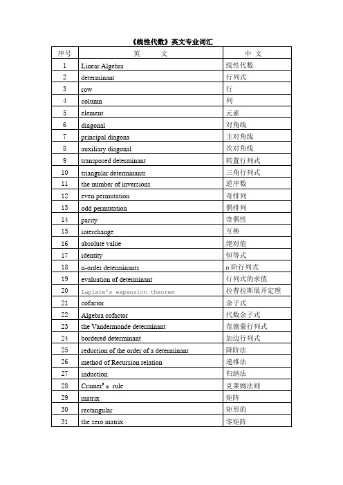
《线性代数》英文专业词汇
序号
英文
中 文
1
Linear Algebra
线性代数
2
determinant
行列式
3
row
行
4
column
列
5
element
元素
6
diagonal
对角线
7
principal diagona
主对角线
8
auxiliary diagonal
次对角线
9
transposed determinant
78
augmented matrix
增广矩阵
79
general solution
数学专业外文翻译--多元函数的极值
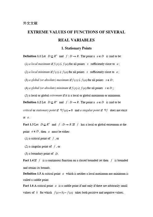
外文文献EXTREME VALUES OF FUNCTIONS OF SEVERALREAL VARIABLES1. Stationary PointsDefinition 1.1 Let n R D ⊆ and R D f →:. The point a D a ∈ is said to be:(1) a local maximum if )()(a f x f ≤for all points x sufficiently close to a ;(2) a local minimum if )()(a f x f ≥for all points x sufficiently close to a ;(3) a global (or absolute) maximum if )()(a f x f ≤for all points D x ∈;(4) a global (or absolute) minimum if )()(a f x f ≥for all points D x ∈;;(5) a local or global extremum if it is a local or global maximum or minimum. Definition 1.2 Let n R D ⊆ and R D f →:. The point a D a ∈ is said to be critical or stationary point if 0)(=∇a f and a singular point if f ∇ does not exist at a .Fact 1.3 Let n R D ⊆ and R D f →:.If f has a local or global extremum at the point D a ∈, then a must be either:(1) a critical point of f , or(2) a singular point of f , or(3) a boundary point of D .Fact 1.4 If f is a continuous function on a closed bounded set then f is bounded and attains its bounds.Definition 1.5 A critical point a which is neither a local maximum nor minimum is called a saddle point.Fact 1.6 A critical point a is a saddle point if and only if there are arbitrarily small values of h for which )()(a f h a f -+ takes both positive and negative values.Definition 1.7 If R R f →2: is a function of two variables such that all second order partial derivatives exist at the point ),(b a , then the Hessian matrix of f at ),(b a is the matrix⎪⎪⎭⎫ ⎝⎛=yy yxxy xx f f f f H where the derivatives are evaluated at ),(b a . If R R f →3: is a function of three variables such that all second order partial derivatives exist at the point ),,(c b a , then the Hessian of f at ),,(c b a is the matrix⎪⎪⎪⎭⎫ ⎝⎛=zz zy zx yz yy yx xz xy xx f f f f f f f f f H where the derivatives are evaluated at ),,(c b a .Definition 1.8 Let A be an n n ⨯ matrix and, for each n r ≤≤1,let r A be the r r ⨯ matrix formed from the first r rows and r columns of A .The determinants det(r A ),n r ≤≤1,are called the leading minors of ATheorem 1.9(The Leading Minor Test). Suppose that R R f →2:is a sufficiently smooth function of two variables with a critical point at ),(b a and H the Hessian of f at ),(b a .If 0)det(≠H , then ),(b a is:(1) a local maximum if 0>det(H 1) = f xx and 0<det(H )=2xy yy xx f f f -;(2) a local minimum if 0<det(H 1) = f xx and 0<det(H )=2xy yy xx f f f -;(3) a saddle point if neither of the above hold.where the partial derivatives are evaluated at ),(b a .Suppose that R R f →3: is a sufficiently smooth function of three variables with a critical point at ),,(c b a and Hessian H at ),,(c b a .If 0)det(≠H , then ),,(c b a is:(1) a local maximum if 0>det(H 1), 0<det(H 2) and 0>det(H 3);(2) a local minimum if 0<det(H 1), 0<det(H 2) and 0>det(H 3);(3) a saddle point if neither of the above hold.where the partial derivatives are evaluated at ),,(c b a .In each case, if det(H )= 0, then ),(b a can be either a local extremum or a saddleExample. Find and classify the stationary points of the following functions:(1) ;1),,(2224+++++=xz z y y x x z y x f(2) ;)1()1(),(422++++=x y x y y x fSolution. (1) 1),,(2224+++++=xz z y y x x z y x f ,so)24),(3z xy x y x f ++=∇(i )2(2y x ++j )2(x z ++kCritical points occur when 0=∇f ,i.e. when(1) z xy x ++=2403(2) y x 202+=(3) x z +=20Using equations (2) and (3) to eliminate y and z from (1), we see that 021433=--x x x or 0)16(2=-x x ,giving 0=x ,66=x and 66-=x .Hence we have three stationary points: )(0,0,0,)(126,121,66-- and )(126,121,66--. Since y x f xx 2122+=,x f xy 2=,1=xz f ,2=yy f ,0=yz f and 2=zz f ,the Hessian matrix is⎪⎪⎪⎭⎫ ⎝⎛+=201022122122x x y x H At )(126,121,66--, ⎪⎪⎪⎪⎭⎫ ⎝⎛=201023/613/66/11H which has leading minors 611>0, 039631123/63/66/11det >=-=⎪⎪⎭⎫ ⎝⎛ And det 042912322>=--=H .By the Leading Minor Test, then, )(126,121,66--is a local minimum. At )(126,121,66--, ⎪⎪⎪⎪⎭⎫ ⎝⎛--=201023/613/66/11H which has leading minors 611>0,039631123/63/66/11det >=-=⎪⎪⎭⎫ ⎝⎛ And det 042912322>=--=H .By the Leading Minor Test, then, )(126,121,66--is also a local minimum. At )(0,0,0, the Hessian is⎪⎪⎪⎭⎫ ⎝⎛=201020100HSince det 2)(-=H , we can apply the leading minor test which tells us that this is a saddle point since the first leading minor is 0. An alternative method is as follows. In this case we consider the value of the expressionhl l k k h h l k h f f D ++++=+++-=22240,0,00,0,0)()(,for arbitrarily small values of h, k and l. But for very small h, k and l , cubic terms and above are negligible in comparison to quadratic and linear terms, sothat hl l k D ++≈22.If h, k and l are all positive, 0>D . However, if 0=k and 0<h and h l <<0,then 0<D .Hence close to )(0,0,0,f both increases and decreases, so )(0,0,0 is a saddle point.(2) 422)1()1(),(++++=x y x y y x f so))1(4)1(2(),(3+++=∇x y x y x f i ))1(2(2+++x y j .Stationary points occur when 0=∇f ,i.e. at )0,1(-.Let us classify this stationary point without considering the Leading Minor Test (in this case the Hessian has determinant 0 at )0,1(- so the test is not applicable). Let.0,10,1422h k h k k h f f D ++=++---=)()(Completing the square we see that .43)2(222h h k D ++=So for any arbitrarily small values of h and k , that are not both 0, 0>D and we see that f has a local maximum at )0,1(-.2. Constrained Extrema and Lagrange MultipliersDefinition 2.1 Let f and g be functions of n variables. An extreme value of f (x )subject to the condition g (x) = 0, is called a constrained extreme value and g (x ) = 0 is called the constraint.Definition 2.2 If R R f n →: is a function of n variables, the Lagrangian function of f subject to the constraint 0),,,(21=n x x x g is the function of n+1 variables),,,,(),,,(),,,,(212121n n n x x x g x x x f x x x L λλ+=where is known as the Lagrange multiplier.The Lagrangian function of f subject to the k constraints0),,,(21=n i x x x g ,k i ≤≤1, is the function with k Lagrange multipliers,i λk i ≤≤1,∑=+=ki n n n x x x g x x x f x x x L 1212121),,,(),,,(),,,,( λλTheorem 2.3 Let R R f →2: and ),(00y x P = be a point on the curve C, withequation g(x,y) = 0, at which f restricted to C has a local extremum.Suppose that both f and g have continuous partial derivatives near to P and that P is not an end point of C and that 0),(00≠∇y x g . Then there is some λ such that ),,(000z y x is a critical point of the Lagrangian Function),(),(),,(y x g y x f y x L λλ+=.Proof. Sketch only. Since P is not an end point and 0≠∇g ,C has a tangent at P with normal g ∇.If f ∇ is not parallel to g ∇at P , then it has non-zero projection along this tangent at P .But then f increases and decreases away from P along C ,so P is not an extremum. Hence f ∇and g ∇are parallel and there is some¸such that g f ∇-=∇λ and the result follows.Example. Find the rectangular box with the largest volume that fits inside the ellipsoid 1222222=++cz b y a x ,given that it sides are parallel to the axes. Solution. Clearly the box will have the greatest volume if each of its corners touch the ellipse. Let one corner of the box be corner (x, y, z) in the positive octant, then the box has corners (±x,±y,±z) and its volume is V= 8xyz .We want to maximize V given that 01222222=-++cz b y a x . (Note that since the constraint surface is bounded a max/min does exist). The Lagrangian is⎪⎪⎭⎫ ⎝⎛-+++=18),,,(222222c z b y a x xyz z y x L λλ and this has critical points when 0=∇L , i.e. when,.280,28022b y zx y L a x yz x L λλ+=∂∂=+=∂∂=⎪⎪⎭⎫ ⎝⎛-++=∂∂=+=∂∂=10,2802222222c z b y a x z L c z xy z L λ (Note that λL will always be the constraint equation.) As we want to maximize V we can assume that 0≠xyz so that 0,,≠z y x .)Hence, eliminating λ, we get,444222zxy c y zx b x yz a -=-=-=λ so that 2222b x a y = and .2222c y b z =But then 222222c z b y a x ==so 2222222231ax c z b y a x =++= or 3a x =,which implies that 3b y = and 3c z = (they are all positive by assumption). So L has only one stationary point ),3,3,3(λc b a (for some value of λ, which we could work out if we wanted to). Since it is the only stationary point it must the required max and the max volume is3383338abc c b a =.中文译文 多元函数的极值1. 稳定点定义1.1 使n R D ⊆并且R D f →:. 对于任意一点D a ∈有以下定义:(1)如果)()(a f x f ≤对于所有x 充分地接近a 时,则)(a f 是一个局部极大值;(2)如果)()(a f x f ≥对于所有x 充分地接近a 时,则)(a f 是一个局部极小值;(3)如果)()(a f x f ≤对于所有点D x ∈成立,则)(a f 是一个全局极大值(或绝对极大值);(4) 如果)()(a f x f ≥对于所有点D x ∈成立,则)(a f 是一个全局极小值(或绝对极小值); (5) 局部极大(小)值统称为局部极值;全局极大(小)值统称为全局极值.定义 1.2 使n R D ⊆并且R D f →:.对于任意一点D a ∈,如果0)(=∇a f ,并且对于任意奇异点a 都不存在f ∇,则称a 是一个关键点或稳定点.结论 1.3 使n R D ⊆并且R D f →:.如果f 有局部极值或全局极值对于一点D a ∈, 则a 一定是:(1)函数f 的一个关键点, 或者(2)函数f 的一个奇异点, 或者(3)定义域D 的一个边界点.结论 1.4 如果函数f 是一个在闭区间上的连续函数,则f 在区间上有边界并且可以取到边界值.定义 1.5 对于任一个关键点a ,当a 既不是局部极大值也不是局部极小值时,a 叫做函数的鞍点.结论 1.6 对于一个关键点a 是鞍点当且仅当h 任意小时,对于函数)()(a f h a f -+取正值和负值.定义 1.7 如果R R f →2: 是二元函数,并且在点),(b a 处所有二阶偏导数都存在,则则根据函数f 在点),(b a 处导数,有f 在点),(b a 处的Hessian 矩阵为:⎪⎪⎭⎫ ⎝⎛=yy yx xy xxf ff f H . 推广:如果R R f →3: 是三元函数,并且在点),,(c b a 处所有二阶偏导数都存在,则根据函数f 在点),,(c b a 处导数,有f 在点),,(c b a 处的Hessian 矩阵为:⎪⎪⎪⎭⎫ ⎝⎛=zz zyzxyz yy yxxz xy xxf f f f f f f f f H . 定义 1.8 矩阵A 是n n ⨯ 阶矩阵,并且对于每一个都有n r ≤≤1,从矩阵A 中选取左上端的r 行和r 列,令其为r r ⨯阶的矩阵r A .则行列式det(r A ),n r ≤≤1,叫做矩阵A 的顺序主子式.定理 1.9 假如R R f →2:是一个充分光滑的二元函数,且在点),(b a 处稳定,其Hessian 矩阵为H .如果0)det(≠H ,则根据偏导数判定),(b a 点是:(1) 一个局部极大值点, 如果0>det(H 1) = f xx 并且0<det(H )=2xy yy xx f f f -; (2) 一个局部极小值点, 如果0<det(H 1) = f xx 并且0<det(H )=2xy yy xx f f f -;(3) 一个鞍点,如果点),(b a 既不是局部极大值点也不是局部极小值点. 假如R R f →3:是一个充分光滑的三元函数,且在点),,(c b a 处稳定,其Hessian 矩阵为H .如果0)det(≠H ,则根据偏导数判定),,(c b a 点是: (1) 一个局部极大值点, 如果当0>det(H 1), 0<det(H 2) 并且 0>det(H 3)时; (2) 一个局部极小值点, 如果当0<det(H 1), 0<det(H 2) 并且 0>det(H 3)时; (3) 一个鞍点,如果点),,(c b a 既不是局部极大值点也不是局部极小值点. 在不同的情况下 ,当det(H )= 0时, 点),(b a 是一个局部极值点,或者是一个鞍点.例. 确定下列函数的稳定点并说明是哪一类点: (1) ;1),,(2224+++++=xz z y y x x z y x f (2) ;)1()1(),(422++++=x y x y y x f 解. (1) 1),,(2224+++++=xz z y y x x z y x f ,so)24),(3z xy x y x f ++=∇(i )2(2y x ++j )2(x z ++k当0=∇f 时有稳定点,也就是说, 当(1) z xy x ++=2403 (2) y x 202+= (3) x z +=20时,将方程(2)和方程(3)带入到方程(1)可以消去变量y 和z, 由此可以得到021433=--x x x 即0)16(2=-x x ,得0=x ,66=x 和66-=x .因此我们可以得到函数的三个稳定点:)(0,0,0,)(126,121,66--和)(126,121,66--. 又因为y x f xx 2122+=,x f xy 2=,1=xz f ,2=yy f ,0=yz f 和2=zz f ,则Hessian 矩阵为⎪⎪⎪⎭⎫⎝⎛+=201022122122x x y x H在点)(126,121,66--处, ⎪⎪⎪⎪⎭⎫⎝⎛=201023/613/66/11H则顺序主子式611>0, 039631123/63/66/11>=-=并且行列式042912322>=--=H .根据主子式判定方法,则点)(126,121,66--是一个局部极小值点.在点)(126,121,66--处, ⎪⎪⎪⎪⎭⎫ ⎝⎛--=201023/613/66/11H则顺序主子式 611>0,039631123/63/66/11>=-=-- 并且行列式042912322>=--=H .根据主子式判定方法,则点)(126,121,66--也是一个极小值点.在点)(0,0,0处,Hessian 矩阵为⎪⎪⎪⎭⎫⎝⎛=201020100H因此det 2)(-=H ,根据主子式判定方法,第一主子式为0,由此我们可以知道该点是一个鞍点. 下面是另一种计算方法,在这种情况下,我们考虑现在下面函数表达式hl l k k h h l k h f f D ++++=+++-=22240,0,00,0,0)()(,的值,对于任意h, k 和l 无限小时. 担当h, k 和l 非常小时, 三次及三次以上方程相对线性二次方程时可忽略不计,则原方程可为hl l k D ++≈22.当h, k 和l 都为正时,0>D .然而, 当0=k 、0<h 和h l <<0,则0<D .因此当接近)(0,0,0时,f 同时增加或者同时减少, 所以 )(0,0,0是一个鞍点. (2) 422)1()1(),(++++=x y x y y x f so))1(4)1(2(),(3+++=∇x y x y x f i ))1(2(2+++x y j .当0=∇f 时有稳定点,也就是说, 当在)0,1(-时.现在我们在不考虑主子式判定方法的情况下为该稳定点进行分类(因为在)0,1(-时Hessian 矩阵的行列式为0,所以该判定方法在此刻无法应用).令.0,10,1422h k h k k h f f D ++=++---=)()(配成完全平方的形式为.43)2(222h h k D ++=所以对h 和k 为任意小时(h 和k 都不为0),有0>D ,因此我们可以确定函数f 在点)0,1(-处有局部极大值.2. 条件极值和Lagrange 乘数法定义 2.1 函数f 和函数g 都是n 元函数.对于限制在条件g (x) = 0下的函数f (x )的极值叫做函数的条件极值,函数g (x ) = 0叫做限制条件.定义 2.2 如果函数R R f n →: 是一个n 元函数, 则对应于函数f 的Lagrange 函数在限制条件0),,,(21=n x x x g 下的函数是一个n +1元函数),,,,(),,,(),,,,(212121n n n x x x g x x x f x x x L λλ+=这就是著名的Lagrange 乘数法.对应于函数f 的Lagrange 函数在k 个限制条件0),,,(21=n i x x x g ,k i ≤≤1时, 带有k 个i λk i ≤≤1,的Lagrange 函数为:∑+=kn n n x x x g x x x f x x x L 212121),,,(),,,(),,,,( λλ定理 2.3 使R R f →2:并且),(00y x P =是曲线C 上的一个点, 有方程 g(x,y) = 0成立,则在限制条件C 上函数f 有局部极值.假设函数f 和函数g 在点P 都有连续的偏导数,点P 不是曲线C 的端点,且0),(00≠∇y x g . 因此存在λ的值使得点),,(000z y x 是Lagrange 函数的关键点),(),(),,(y x g y x f y x L λλ+=.证明.仅仅描述. 因为点P 不是曲线C 的端点,且0≠∇g ,则曲线C 在点P 处的切线与g ∇有关.如果f ∇在点P 处与g ∇平行,则函数在点P 处的切线有非零值.但另一方面函数 f 的值随着P 在C 的运动增加减小,所以点P 不是极值点. 因为f ∇和g ∇平行,所以存在λ使得g f ∇-=∇λ成立.例. 求内接于椭球1222222=++cz b y a x 的体积最大的长方体的体积,长方体的各个面平行于坐标面解:明显地,当长方体的体积最大时,长方体的各个顶点一定在椭球上. 设长方体的一个顶点坐标为(x, y, z) (x>0, y>0, z>0), 则长方体的其他顶点坐标分别为(±x,±y,±z),并且长方体的体积为V= 8xyz.我们要求V 在条件01222222=-++cz b y a x 下的最大值. (注意:因为约束条件是有边界的,故其一定存在极大或者极小值). 其Lagrange 函数为⎪⎪⎭⎫⎝⎛-+++=18),,,(222222c z b y a x xyz z y x L λλ并且存在稳定点当0=∇L 时,也就是说,当,.280,280,280222cz xy z L b yzx y L a x yz x L λλλ+=∂∂=+=∂∂=+=∂∂=⎪⎪⎭⎫ ⎝⎛-++=∂∂=10222222c z b y a x z L 时.(注意:λL 是约束方程.要想求得体积V 的最大值,假设0≠xyz ,则可得0,,≠z y x .)因此, 用其他式子表示λ, 我们可以得到,444222zxyc y zx b x yz a -=-=-=λ 消去λ,有2222b x a y =和.2222c y b z =进而得出 222222cz b y a x ==,因此有2222222231ax c z b y a x =++=或者得出3a x =,同理可得出3by =和3c z = (根据假设可得x, y, z 都是正值).所以函数 L 有且仅有一个稳定点),3,3,3(λc b a (λ为某一计算可得到的常数). 又因为该点是函数L 的唯一稳定点,则该稳定点一定是所要求的最大值点,故其体积的最大值为3383338abcc b a =.。
数据分析外文文献+翻译
数据分析外文文献+翻译文献1:《数据分析在企业决策中的应用》该文献探讨了数据分析在企业决策中的重要性和应用。
研究发现,通过数据分析可以获取准确的商业情报,帮助企业更好地理解市场趋势和消费者需求。
通过对大量数据的分析,企业可以发现隐藏的模式和关联,从而制定出更具竞争力的产品和服务策略。
数据分析还可以提供决策支持,帮助企业在不确定的环境下做出明智的决策。
因此,数据分析已成为现代企业成功的关键要素之一。
文献2:《机器研究在数据分析中的应用》该文献探讨了机器研究在数据分析中的应用。
研究发现,机器研究可以帮助企业更高效地分析大量的数据,并从中发现有价值的信息。
机器研究算法可以自动研究和改进,从而帮助企业发现数据中的模式和趋势。
通过机器研究的应用,企业可以更准确地预测市场需求、优化业务流程,并制定更具策略性的决策。
因此,机器研究在数据分析中的应用正逐渐受到企业的关注和采用。
文献3:《数据可视化在数据分析中的应用》该文献探讨了数据可视化在数据分析中的重要性和应用。
研究发现,通过数据可视化可以更直观地呈现复杂的数据关系和趋势。
可视化可以帮助企业更好地理解数据,发现数据中的模式和规律。
数据可视化还可以帮助企业进行数据交互和决策共享,提升决策的效率和准确性。
因此,数据可视化在数据分析中扮演着非常重要的角色。
翻译文献1标题: The Application of Data Analysis in Business Decision-making The Application of Data Analysis in Business Decision-making文献2标题: The Application of Machine Learning in Data Analysis The Application of Machine Learning in Data Analysis文献3标题: The Application of Data Visualization in Data Analysis The Application of Data Visualization in Data Analysis翻译摘要:本文献研究了数据分析在企业决策中的应用,以及机器研究和数据可视化在数据分析中的作用。
二维码中英文对照外文翻译文献

二维码中英文对照外文翻译文献(文档含英文原文和中文翻译)译文:在印刷广告中二维码使用:阐明印度时尚使用内容分析1.介绍全球移动电话的普及率已经爆炸,已经触及86.7%的马克(暴徒想,2011)。
高普及率是手机的商业潜力的指标,这也就不足为奇了营销人员手机感兴趣看成是一种广告媒介(Wohlfahrt,2002)。
这个移动平台提供了多样化的模式,即匹配所需的通信。
SMS(短消息服务),MMS(多媒体通讯服务)、移动视频、WAP(无线访问协议)等(Beschizza,2009)。
甚至手机的具体特征像区域定位能力(通过全球定位系统和细胞的起源),普遍、直接、可测性和交互性支持手机在营销传播中的应用(鲍尔et al .,2005;Haghirian et al .,2005)。
此外,在过去的几年中,手机在日常生活中得到了越来越多的重要性的消费者因此这使得营销人员最简单的方式与他们交流(Pelu Zegreanu,2010)。
当然,这些进步有注意人员和营销人员对各种类型的基于手机的营销策略(Wohlfahrt,2002;Trappey伍德赛德,2005;戴维斯和Sajtos,2008)。
这样的营销战术工具快速响应代码,通常缩写为二维码(参见图1),二维码是2维条形码(数据矩阵)旨在被智能手机摄像头扫描,结合条形码解码应用程序(Denso-wave,无日期)。
各种这样的应用程序可以像QuickMark、Scanlife RedLaser,i-nigma,QRreader将用户连接到一些特定的电子内容像一个网站,一个电子邮件地址,支付系统,短信,一个注册表单等等。
(无人看顾,2012;Bisel,2012)。
二维码被日本电装波第一概念化,1994年在日本丰田子公司。
正常的条形码信息存储在只有一维(横向)和严重限制在他们可以包含的数据量。
日本电装波开发这个二维码的方式持有信息两个维度(横向和纵向);因此二维码能够积累更多的信息比一个正常的10倍条形码(Denso-wave,无日期)。
数学 外文翻译 外文文献 英文文献 具体数学
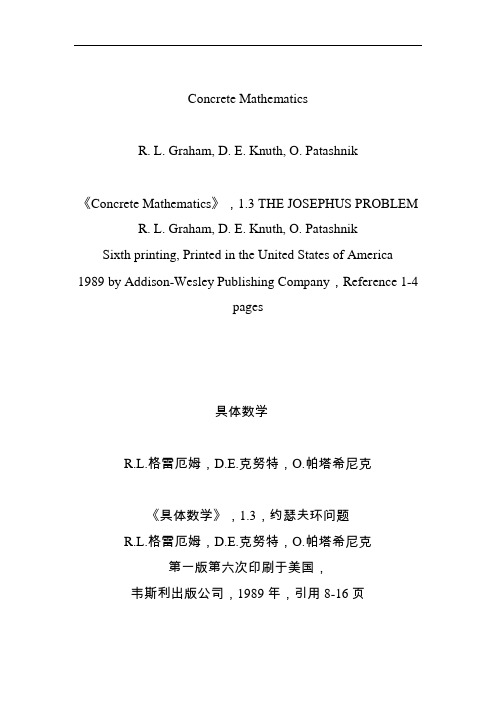
Concrete MathematicsR. L. Graham, D. E. Knuth, O. Patashnik《Concrete Mathematics》,1.3 THE JOSEPHUS PROBLEM R. L. Graham, D. E. Knuth, O. Patashnik Sixth printing, Printed in the United States of America 1989 by Addison-Wesley Publishing Company,Reference 1-4pages具体数学R.L.格雷厄姆,D.E.克努特,O.帕塔希尼克《具体数学》,1.3,约瑟夫环问题R.L.格雷厄姆,D.E.克努特,O.帕塔希尼克第一版第六次印刷于美国,韦斯利出版公司,1989年,引用8-16页1.递归问题本章研究三个样本问题。
这三个样本问题给出了递归问题的感性知识。
它们有两个共同的特点:它们都是数学家们一直反复地研究的问题;它们的解都用了递归的概念,按递归概念,每个问题的解都依赖于相同问题的若干较小场合的解。
2.约瑟夫环问题我们最后一个例子是一个以Flavius Josephus命名的古老的问题的变形,他是第一世纪一个著名的历史学家。
据传说,如果没有Josephus的数学天赋,他就不可能活下来而成为著名的学者。
在犹太|罗马战争中,他是被罗马人困在一个山洞中的41个犹太叛军之一,这些叛军宁死不屈,决定在罗马人俘虏他们之前自杀,他们站成一个圈,从一开始,依次杀掉编号是三的倍数的人,直到一个人也不剩。
但是在这些叛军中的Josephus和他没有被告发的同伴觉得这么做毫无意义,所以他快速的计算出他和他的朋友应该站在这个恶毒的圆圈的哪个位置。
在我们的变形了的问题中,我们以n个人开始,从1到n编号围成一个圈,我们每次消灭第二个人直到只剩下一个人。
例如,这里我们以设n= 10做开始。
外文参考文献及翻译稿的要求与格式
百度文库- 让每个人平等地提升自我!外文参考文献及翻译稿的要求及格式一、外文参考文献的要求1、外文原稿应与本研究项目接近或相关联;2、外文原稿可选择相关文章或节选章节,正文字数不少于1500字。
3、格式:外文文献左上角标注“外文参考资料”字样,小四宋体。
1.5倍行距。
标题:三号,Times New Roman字体加粗,居中,行距1.5倍。
段前段后空一行。
作者(居中)及正文:小四号,Times New Roman字体,首行空2字符。
4、A4纸统一打印。
二、中文翻译稿1、中文翻译稿要与外文文献匹配,翻译要正确;2、中文翻译稿另起一页;3、格式:左上角标“中文译文”,小四宋体。
标题:宋体三号加粗居中,行距1.5倍。
段前、段后空一行。
作者(居中)及正文:小四号宋体,数字等Times New Roman字体,1.5倍行距,首行空2字符。
正文字数1500左右。
4、A4纸统一打印。
格式范例如后所示。
百度文库 - 让每个人平等地提升自我!外文参考文献Implementation of internal controls of small andmedium-sized pow erStephen Ryan The enterprise internal control carries out the strength to refer to the enterprise internal control system execution ability and dynamics, it is the one whole set behavior and the technical system, is unique competitive advantage which the enterprise has; Is a series of …………………………标题:三号,Times New Roman字体加粗,居中,行距1.5倍。
- 1、下载文档前请自行甄别文档内容的完整性,平台不提供额外的编辑、内容补充、找答案等附加服务。
- 2、"仅部分预览"的文档,不可在线预览部分如存在完整性等问题,可反馈申请退款(可完整预览的文档不适用该条件!)。
- 3、如文档侵犯您的权益,请联系客服反馈,我们会尽快为您处理(人工客服工作时间:9:00-18:30)。
Assume that you have a guess U(n) of the solution. If U(n) is close enough to the exact solution, an improved approximation U(n + 1) is obtained by solving the linearized problemwhere have asolution.has. In this case, the Gauss-Newton iteration tends to be the minimizer of the residual, i.e., the solution of minUIt is well known that for sufficiently smallAndis called a descent direction for , where | is the l2-norm. The iteration iswhere is chosen as large as possible such that the step has a reasonable descent.The Gauss-Newton method is local, and convergence is assured only when U(0)is close enough to the solution. In general, the first guess may be outside thergion of convergence. To improve convergence from bad initial guesses, a damping strategy is implemented for choosing , the Armijo-Goldstein line search. It chooses the largestinequality holds:|which guarantees a reduction of the residual norm by at least Note that each step of the line-search algorithm requires an evaluation of the residualAn important point of this strategy is that when U(n) approaches the solution, then and thus the convergence rate increases. If there is a solution to the scheme ultimately recovers the quadratic convergence rate of the standard Newton iteration. Closely related to the above problem is the choice of the initial guess U(0). By default, the solver sets U(0) and then assembles the FEM matrices K and F and computesThe damped Gauss-Newton iteration is then started with U(1), which should be a better guess than U(0). If the boundary conditions do not depend on the solution u, then U(1) satisfies them even if U(0) does not. Furthermore, if the equation is linear, then U(1) is the exact FEM solution and the solver does not enter the Gauss-Newton loop.There are situations where U(0) = 0 makes no sense or convergence is impossible.In some situations you may already have a good approximation and the nonlinear solver can be started with it, avoiding the slow convergence regime.This idea is used in the adaptive mesh generator. It computes a solution on a mesh, evaluates the error, and may refine certain triangles. The interpolant of is a very good starting guess for the solution on the refined mesh.In general the exact Jacobianis not available. Approximation of Jn by finite differences in the following way is expensive but feasible. The ith column of Jn can be approximated bywhich implies the assembling of the FEM matrices for the triangles containing grid point i. A very simple approximation to Jn, which gives a fixed point iteration, is also possible as follows. Essentially, for a given U(n), compute the FEM matrices K and F and setNonlinear EquationsThis is equivalent to approximating the Jacobian with the stiffness matrix. Indeed, since putting Jn = K yields In many cases the convergence rate is slow, but the cost of each iteration is cheap.The nonlinear solver implemented in the PDE Toolbox also provides for a compromise between the two extremes. To compute the derivative of the mapping , proceed as follows. The a term has been omitted for clarity, but appears again in the final result below.The first integral term is nothing more than Ki,j.The second term is “lumped,” i.e., replaced by a diagonal matrix that contains the row j j = 1, the second term is approximated bywhich is the ith component of K(c')U, where K(c') is the stiffness matrixassociated with the coefficient rather than c. The same reasoning can beapplied to the derivative of the mapping . Finally note that thederivative of the mapping is exactlywhich is the mass matrix associated with the coefficient . Thus the Jacobian ofU) is approximated bywhere the differentiation is with respect to u. K and M designate stiffness and mass matrices and their indices designate the coefficients with respect to which they are assembled. At each Gauss-Newton iteration, the nonlinear solver assembles the matrices corresponding to the equationsand then produces the approximate Jacobian. The differentiations of the coefficients are done numerically.In the general setting of elliptic systems, the boundary conditions are appended to the stiffness matrix to form the full linear system: where the coefficients of and may depend on the solution . The “lumped”approach approximates the derivative mapping of the residual by The nonlinearities of the boundary conditions and the dependencies of the coefficients on the derivatives of are not properly linearized by this scheme. When such nonlinearities are strong, the scheme reduces to the fix-pointiter ation and may converge slowly or not at all. When the boundary condition sare linear, they do not affect the convergence properties of the iteration schemes. In the Neumann case they are invisible (H is an empty matrix) and in the Dirichlet case they merely state that the residual is zero on the corresponding boundary points.Adaptive Mesh RefinementThe toolbox has a function for global, uniform mesh refinement. It divides each triangle into four similar triangles by creating new corners at the midsides, adjusting for curved boundaries. You can assess the accuracy of the numerical solution by comparing results from a sequence of successively refined meshes.If the solution is smooth enough, more accurate results may be obtained by extra polation. The solutions of the toolbox equation often have geometric features like localized strong gradients. An example of engineering importance in elasticity is the stress concentration occurring at reentrant corners such as the MATLAB favorite, the L-shaped membrane. Then it is more economical to refine the mesh selectively, i.e., only where it is needed. When the selection is based ones timates of errors in the computed solutions, a posteriori estimates, we speak of adaptive mesh refinement. Seeadapt mesh for an example of the computational savings where global refinement needs more than 6000elements to compete with an adaptively refined mesh of 500 elements.The adaptive refinement generates a sequence of solutions on successively finer meshes, at each stage selecting and refining those elements that are judged to contribute most to the error. The process is terminated when the maximum number of elements is exceeded or when each triangle contributes less than a preset tolerance. You need to provide an initial mesh, and choose selection and termination criteria parameters. The initial mesh can be produced by the init mesh function. The three components of the algorithm are the error indicator function, which computes an estimate of the element error contribution, the mesh refiner, which selects and subdivides elements, and the termination criteria.The Error Indicator FunctionThe adaption is a feedback process. As such, it is easily applied to a lar gerrange of problems than those for which its design was tailored. You wantes timates, selection criteria, etc., to be optimal in the sense of giving the mostaccurate solution at fixed cost or lowest computational effort for a given accuracy. Such results have been proved only for model problems, butgenerally, the equid is tribution heuristic has been found near optimal. Element sizes should be chosen such that each element contributes the same to the error. The theory of adaptive schemes makes use of a priori bounds forsolutions in terms of the source function f. For none lli ptic problems such abound may not exist, while the refinement scheme is still well defined and has been found to work well.The error indicator function used in the toolbox is an element-wise estimate of the contribution, based on the work of C. Johnson et al. For Poisson'sequation –f -solution uh holds in the L2-normwhere h = h(x) is the local mesh size, andThe braced quantity is the jump in normal derivative of v hr is theEi, the set of all interior edges of thetrain gulation. This bound is turned into an element-wise error indicator function E(K) for element K by summing the contributions from its edges. The final form for the toolbox equation Becomeswhere n is the unit normal of edge and the braced term is the jump in flux across the element edge. The L2 norm is computed over the element K. This error indicator is computed by the pdejmps function.The Mesh RefinerThe PDE Toolbox is geared to elliptic problems. For reasons of accuracy and ill-conditioning, they require the elements not to deviate too much from beingequilateral. Thus, even at essentially one-dimensional solution features, such as boundary layers, the refinement technique must guarantee reasonably shaped triangles.When an element is refined, new nodes appear on its mid sides, and if the neighbor triangle is not refined in a similar way, it is said to have hanging nodes. The final triangulation must have no hanging nodes, and they are removed by splitting neighbor triangles. To avoid further deterioration oftriangle quality in successive generations, the “longest edge bisection” scheme Rosenberg-Stenger [8] is used, in which the longest side of a triangle is always split, whenever any of the sides have hanging nodes. This guarantees that no angle is ever smaller than half the smallest angle of the original triangulation. Two selection criteria can be used. One, pdead worst, refines all elements with value of the error indicator larger than half the worst of any element. The other, pdeadgsc, refines all elements with an indicator value exceeding a user-defined dimensionless tolerance. The comparison with the tolerance is properly scaled with respect to domain and solution size, etc.The Termination CriteriaFor smooth solutions, error equi distribution can be achieved by the pde adgsc selection if the maximum number of elements is large enough. The pdead worst adaption only terminates when the maximum number of elements has been exceeded. This mode is natural when the solution exhibits singularities. The error indicator of the elements next to the singularity may never vanish, regardless of element size.外文翻译假定估计值,如果是最接近的准确的求解,通过解决线性问题得到更精确的值当为正数时,( 有一个解,即使也有一个解都是不需要的。