An O(n log n) Algorithm for the all nearest neighbors problem

合集下载

后现代叙事理论_英文_

Postmodern Narrative TheoryB rian R ichardsonAbst ract:In this article I descri b e so m e basic features of post m oder n narrative,note its differ ences fr o m other,m i m etic types o f narrati v e,and identify the k i n d of theoretica l fra m e wo r k neces sar y to co mprehend such w orks.I beg in w ith a general account o f the disti n cti v e nature of post m oder n narrati v e,and then d iscuss t h e re lations a mong authors,i m p lied authors,and narrators in trad iti o na l and post m oder n narrati v es.I iden tify characteristic post m odern strateg ies,inc l u d i n g t h e use o fm ultiple k i n ds of narrato rs,second person narrati o n,and var i o us for m s o f i m possi b le narrati o n.I then m ove on to ti m e,p lo,t and progressi o n,and again i d entify a number o f d istinc ti v e post m oder n strateg ies,such as the use of unusual or unnatural stories,i m possible chronolo gies,denarrati o n,and nontraditi o na l end i n gs.Throughout the essay I prov ide exa m ples fro m Sa l m an Rushd ie s M idnigh t s Chil d ren and o ther post m oder n texts to ill u strate these concepti o ns. K ey w ords:narrati o n narrator post m odernis m pr ogressi o n story ti m eAut hor:Brian R ichardson is a Professo r i n t h e Eng li s h Depart m ent of the Un iversity o fM ary land,USA.H is i n terests are narrati v e theory,m odernis m,and post m odern is m.H e is the author of Unlikel y Stories:Causalit y and theN ature of M o d ern N arrative(1997)and Unnatural Voices: Ex tre m eN arra tion on M odern and Conte mporary F iction(2006).H e has w ritten num erous arti cles on narrati v e theory.H e is V ice Presi d ent of the I n ter national Society fo r the S t u dy o fN arra ti v e.E m a i:l richb@um 标题:后现代叙事理论内容摘要:本文描述了后现代叙事的基本特征,指出这些特征与其它模仿叙事之间的差异,勾划出解读这些作品所必需的理论框架。

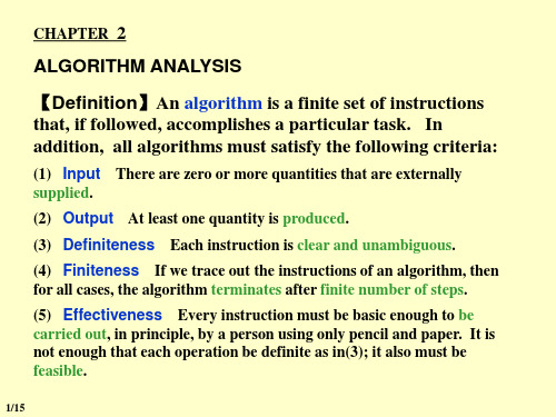
Algorithm-Analysis

I see! So as long as I know that Tp1 is about N2 and Tp2 is about N, then for
sufficiently large N, P2 will be faster!
7/15
§2 Asymptotic Notation
【Definition】 T (N) = O( f (N) ) if there are positive constants c
【Definition】 T (N) = ( h(N) ) if and only if T (N) = O( h(N) ) and
T (N) = ( h(N) ) .
【Definition】 T (N) = o( p(N) ) if T (N) = O( p(N) ) and T (N)
( p(N) ) .
/* count ++ */
return 0; /* count ++ */ }
5/15
§1 What to Analyze
Take the iterative and recursive programs for summing a list for example --- if you think 2n+2 is WTlBStenohIsohuusecytminiott?tdhL’ubswrotayeneheetnhotrtoais’uasiGsolot2tilt’hTtfnya’locdelsswp+soIonrbktte3smdioseehBevxt,etpcrueqpeaheetsetsfsruclhcepsfi.Iy?tas.em?cro.stadsuapahitternotusrieeylUnotidcadsenr’ohereftanfsgdhf!tzooethhy!smrni!t..n.?e..a.ktinmsdoe.s.

A PTAS for the Multiple Knapsack Problem

A PTAS for the Multiple Knapsack ProblemChandra Chekuri Sanjeev KhannaAbstractThe Multiple Knapsack problem(MKP)is a natural and well knowngeneralization of the single knapsack problem and is deﬁned asfollows.We are given a set of items and bins(knapsacks)suchthat each item has a proﬁt and a size,and each bin hasa capacity.The goal is toﬁnd a subset of items of maximumproﬁt such that they have a feasible packing in the bins.MKP is aspecial case of the Generalized Assignment problem(GAP)wherethe proﬁt and the size of an item can vary based on the speciﬁc binthat it is assigned to.GAP is APX-hard and a-approximation for itis implicit in the work of Shmoys and Tardos[26],and thus far,thiswas also the best known approximation for MKP.The main resultof this paper is a polynomial time approximation scheme for MKP.Apart from its inherent theoretical interest as a common gen-eralization of the well-studied knapsack and bin packing problems,it appears to be the strongest special case of GAP that is not APX-hard.We substantiate this by showing that slight generalizationsof MKP are APX-hard.Thus our results help demarcate the bound-ary at which instances of GAP become APX-hard.An interestingand novel aspect of our approach is an approximation preservingreduction from an arbitrary instance of MKP to an instance withdistinct sizes and proﬁts.1IntroductionWe study the following natural generalization of the classicalknapsack problem:Multiple Knapsack Problem(MKP)I NSTANCE:A pair where is a set of bins(knapsacks)and is a set of items.Each bin hasa capacity,and each item has a size and a proﬁt.O BJECTIVE:Find a subset of maximum proﬁt suchthat has a feasible packing in.The decision version of MKP is a generalization of thedecision versions of both the knapsack and bin packingproblems and is strongly NP-Complete.Moreover,it isan important special case of the generalized assignmentproblem where both the size and the proﬁt of an item area function of the bin:1GAP has also been deﬁned in the literature as a(closely related)minimization problem(see[26]).In this paper,following[24],we referto the maximization version of the problem as GAP and refer to theminimization version as Min GAP.item sizes and proﬁts as well as bin capacities may take anyarbitrary values.Establishing a PTAS would show a very ﬁne separation between cases that are APX-hard and thosethat have a PTAS.Until now,the best known approximationratio for MKP was a factor of derived from the approxima-tion for GAP.Our main result:In this paper we resolve the approxima-bility of MKP by obtaining a PTAS for it.It can be easilyshown via a reduction from the Partition problem that MKPdoes not admit a FPTAS even if.A special case of MKP is when all bin capacities are equal.It is relativelystraightforward to obtain a PTAS for this case using ideas from approximation schemes for knapsack and bin packing[11,3,15].However the general case with different bincapacities is a non-trivial and challenging problem.Our paper contains two new technical ideas.Ourﬁrst idea con-cerns the set of items to be packed in a knapsack instance.We show how to guess,in polynomial time,almost all the items that are to be packed in a given knapsack instance.Inother words we can identify an item set that has a feasible packing and proﬁt at least OPT.This is in contrastto earlier schemes for variants of knapsack[11,1,5]whereonly the most proﬁtable items are guessed.An easy corollary of our strategy is a PTAS for the identical bincapacity case,the details of which we point out later.Thestrengthened guessing plays a crucial role in the general case in the following way.As a byproduct of our guessingscheme we show how to round the sizes of items to at most distinct sizes.An immediate consequence of this is a quasi-polynomial time algorithm to pack items intobins using standard dynamic programming.Our second set of ideas shows that we can exploit the restricted sizesto pack,in polynomial time,a subset of the item set thathas at least a fraction of the proﬁt.Approximation schemes for number problems are usually based on rounding instances to have aﬁxed number of distinct values.In contrast,MKP appears to require a logarithmic number of values.We believe that our ideas to handle logarithmic number of distinct values willﬁnd other applications.Figure 1summarizes the approximability of various restrictions of GAP.Related work:MKP is closely related to knapsack,bin packing,and GAP.A very efﬁcient FPTAS exists for the knapsack problem;Lawler[17],based on ideas from[11], achieves a running time of for a approximation.An asymptotic FPTAS is known for bin packing[3,15].Recently Kellerer[16]has independently developed a PTAS for the special case of the MKP where all bins have identical capacity.As mentioned earlier, this case is much simpler than the general case and falls out as a consequence of ourﬁrst idea.The generalized assignment problem,as we phrased it,seeks to maximize proﬁt of items packed.This is natural when viewed as a knapsack problem(see[24]).The minimization version of the problem,referred to as Min GAP and also as the cost assignment problem,seeks to assign all the items while minimizing the sum of the costs of assigning items to bins. In this version,item incurs a cost if assigned to bin instead of a obtaining a proﬁt.Since the feasibility of assigning all items is itself an NP-Complete problem we need to relax the bin capacity constraints.Anbi-criteria approximation algorithm for Min GAP is one that gives a solution with cost at most and with bin capacities violated by a factor of at most where is the cost of an optimal solution that does not violate any capacity constraints.Work of Lin and Vitter[20]yields a approximation for Min GAP.Shmoys and Tardos[26],building on the work of Lenstra,Shmoys, and Tardos[19],give an improved approximation. Implicit in this approximation is also a-approximation for the proﬁt maximization version which we sketch later. Lenstra et al.[19]also show that it is NP-hard to obtain a ratio for any.The hardness relies on a NP-Completeness reduction from3-Dimensional Matching. Our APX-hardness for the maximization version,mentioned earlier,is based on a similar reduction but instead relies on APX-hardness of the optimization version of3-Dimensional matching[14].MKP is also related to two variants of variable size bin packing.In theﬁrst variant we are given a set of items and set of bin capacities.The objective is toﬁnd a feasible packing of items using bins with capacities restricted to be from so as to minimize the sum of the capacities of the bins used.A PTAS for this problem was provided by Murgolo [25].The second variant is based on a connection to multi-processor scheduling on uniformly related machines[18]. The objective is to assign a set of independent jobs with given processing times to machines with different speeds to minimize the makespan of the schedule.Hochbaum and Shymoys[8]gave a PTAS for this problem using a dual based approach where they convert the scheduling problem into the following bin packing problem.Given items of different sizes and bins of different capacities,ﬁnd a packing of all the items into the bins such that maximum violation of the capacity of any bin is minimized. Bi-criteria approximations,where both capacity and proﬁt can be approximated simultaneously,have been studied for several problems(Min GAP being an example mentioned above)and it is usually the case that relaxing both makes the task of approximation somewhat easier.In particular, relaxing the capacity constraints allows rounding of item sizes into a small number of distinct size values.In MKP we are neither allowed to exceed the capacity constraints nor the number of bins.This makes the problem harder and our result interesting.Knapsack GAPMultiple identical capacity binsNo FPTAS even with 2 binsItem size varies with binsvary with bins.Both size and profitMultiple non-identical capacity binsPTAS (special case of Theorem 2.1)2-approximable (Proposition 3.2, [26])if all sizes are identical (Proposition 3.1)However, it is polynomial time solvable only 2 distinct profits (Theorem 3.2)MKPPTAS (Theorem 2.1)(Theorem 3.1)APX-hard even when each item takes Item profit varies with binsFPTAS[10,15]sizes and all profits are identical.each item takes only 2 distinct APX-hard even whenFigure 1:Complexity of Various Restrictions of GAPOrganization:Section 2describes our PTAS for MKP.In Section 3,we show that GAP is APX-hard on very restricted classes of instances.We also indicate here a -approximation for GAP.In Section 4,we discuss a natural greedy algorithmfor MKP and show that it gives a-approximation even when item sizes vary with bins.2A PTAS for the Multiple Knapsack Problem We denote by OPT the value of an optimal solution to thegiven instance.Given a setof items,we use to denote .The set of integers is denoted by .Our problem is related to both the knapsack problem and the bin packing problem and some ideas used in approximation schemes for those problems will be useful to us.Our approximation scheme conceptually has the following two steps.1.G UESSING I TEMS :Identify a set of itemssuch that OPT and has a feasible packing in .2.P ACKING I TEMS :Given a setof items that has a feasible packing in ,ﬁnd a feasible packing for a set such that .The overall scheme is more involved since there is interaction between the two steps.The guessed items have some additional properties that are exploited in the packing step.We observe that both of the above steps require new ideas.For the single knapsack problem no previous algorithm identiﬁes the full set of items to pack.Moreover testing the feasibility of packing a given set of items is trivial.However in MKP the packing step is itself quite complex and it seems necessary to decompose the problem as we did.Before we proceed with the details we show how the ﬁrst step of guessing the items immediately gives a PTAS for the identical bin capacity case.2.1MKP with Identical Bin CapacitiesSuppose we can guess an item set as in our ﬁrst step above.We show that the packing step is very simple if bin capacities are identical.There are two cases to consider depending on whether ,the number of bins,is less than or not.In the former case the number of bins can be treated as a constant and a PTAS for this case exists even for instances of GAP (implicit in earlier work [5]).Now suppose .We use the any of the known PTASs for bin packing andpack all the guessed items using at mostbins.We ﬁnd a feasible solution by simply picking the largest proﬁt bins and discarding the rest along with their items.Here weuse the fact that and that the bins are identical.It is easily seen that we get aapproximation.We note that a different PTAS,without using our guessing step,can be obtained for this case by directly adapting the ideas used in approximation schemes for bin packing.The trick of using extra bins does not have a simple analogue when bin capacities are different and we need more ideas.2.2Guessing ItemsConsider the case when items have the same proﬁt(assume it is).Thus the objective is to pack as many items as possible.For this case it is easily seen that OPT is an integer in.Further,given a guess for OPT,we can always pick the smallest(in size)OPT items to pack.Therefore there are only a polynomial number of guesses for the set of items to pack. This idea does not have a direct extension to non-uniform proﬁts.However the useful insight is that when proﬁts are identical we can pick the items in order of their sizes.In the rest of the paper we assume,for simplicity of notation,that and are integers.For the general case theﬁrst step in guessing items involves massaging the given instance into a more structured one that has few distinct proﬁts.This is accomplished as follows.1.Guess a value such that OPT OPTand discard all items where.2.Scale all proﬁts by such that they are in the range.3.Round down the proﬁts of items to the nearest power of.Theﬁrst two steps are similar to those in the FPTAS for the single knapsack problem.It is easily seen that at most an fraction of the optimal proﬁt is lost by our transformation.Summarizing:L EMMA2.1.Given an instance with items and a value such that OPT OPT we can obtain in polynomial time another instancesuch that.For every,for some.OPTitems.We discard the items in and for each we increase the size of every item in to the size of the smallest item in.Since is ordered by size no item in is larger than the smallest item in for each.It is easy to see that if has a feasible packing then the modiﬁed instance also has a feasible packing.We discard at most an fraction of the proﬁt and the modiﬁed sizes have at most distinct values.Applying this to each proﬁt class we obtain an instance with distinct size values.L EMMA2.3.Given an instance with items we can obtain in polynomial time instances such thatFor,and has items only from distinct proﬁt values.For,and has items only from distinct size values.There exists an index such that has a feasible packing in and OPT.We will assume for the next section that we have guessed the correct set of items and that they are partitioned into sets with each set containing items of the same size.We denote by the items of the th size value and by the quantity.2.3Packing ItemsFrom Lemma2.3we obtain a restricted set of instances in terms of item proﬁts and sizes.We also need some structure in the bins and we start by describing the necessary transformations.2.3.1Structuring the BinsAssume without loss of generality that the smallest bin capacity is.We order the bins in increasing order of their capacity and partition them into blocks such that block consists of all bins with.Let denote the number of bins in block.D EFINITION2.1.(Small rge Blocks)A block of bins is called a small bin block if;it is called large otherwise.Let be the set of indices such that is small.Deﬁne to be the set of largest indices in the set.Let and be the set of all bins in the blocks speciﬁed by the index sets and respectively.The following lemma makes use of the property of geometrically increasing bin capacities.L EMMA2.4.Let be a set of items that can be packed in the bins.There exists a set such that can be packed into the bins,and.Proof.Fix some packing of in the bins.Consider the largest bins in.One of these bins has a proﬁt less than.Without loss of generality assume its capacity is.We will remove the items packed in this bin and use it to pack items from smaller bins.Let be the block containing this bin.Bins in block where andhave a capacity less than.It is easy to verify that the total capacity of bins in small bin blocks with indices less than equal to is at most.Since each of the ﬁrst bins could be in different blocks the upper bound of blocks follows.Therefore we can retain the small bin blocks of large capacity and discard the rest.Therefore we as-sume that the given instance is modiﬁed to satisfy.Then it follows that. When the number of bins isﬁxed a PTAS is known(implicit in earlier work)even for the GAP.We will use ideas from that algorithm.For large bin blocks the advantage is that we can exceed the number of bins used by an fraction,as we shall see below.The main task is to integrate the allocation and packing of items between the different sets of bins.For the rest of the section we assume that we have a set of items that have a feasible packing and we will implicitly refer to someﬁxed feasible packing as the optimal solution.2.3.2Packing Proﬁtable Items into Small Bin Blocks We guess here for each bin in,the most proﬁtable items that are packed in it in the optimal solution.Therefore the number of guesses needed is.2.3.3Packing Large Items into Large Bin BlocksThe second step is to select items and pack them in large bin blocks.We say that an item is packed as a large item if its size is at least times the capacity of the bin in which it is packed.Since the capacities of the blocks are increasing geometrically,an item can be packed as large in at mostCombining for all sizes results in guesses over all.Here is where we take advantage of the fact that our items come from only different size classes.Suppose we have correctly assigned all large items to their respective bin blocks.We describe now a procedure for ﬁnding a feasible packing of these items.Here we ignore the potential interaction between items that are packed as large and those packed as small.We will show later that we can do so with only a slight loss in the approximation factor.We can focus on a speciﬁc block since the large items are now partitioned between the blocks.The abstract problem we have is the following.Given a collection of bins with capacities in the range,and a set of items with sizes in the range,decide if there is a feasible packing for them.It is easily seen that this problem is NP-hard.We obtain a relaxation by allowing use of extra bins to pack the items.However,we restrict the capacity of the extra bins to be.The following algorithm decides that either the given instance is infeasible or gives a packing with at most an additional bins of capacity.Let be the set of items of size greater than.Order items of in non-decreasing sizes and pack each item into the smallest bin available that can accommodate it.Disregard all the bins used up in the previous step since no other large item canﬁt into them.To pack the remaining items use a PTAS for bin pack-ing,potentially using an extra bins of capacity.We omit the full details of the algorithm but summarize the result in the following lemma.L EMMA2.5.Given bins of capacities in the range and items of sizes in the range,there is an algorithm that runs in time,and provided the items have a feasible packing in the given bins,returns a feasible packing using at most extra bins of capacity.We eliminate the extra bins later by picking the most proﬁtable among them and discarding the items packed in the rest.The restriction on the size and number of extra bins is motivated by the elimination procedure.In order to use extra bins the quantity needs to be at least.This is the reason to distinguish between small and large bin blocks.For a large bin block let be the extra bins used in packing the large items.We note that.2.3.4Packing the Remaining ItemsThe third and last step of the algorithm is to pack the remaining items which we denote by.At this stage we have a packing of the most proﬁtable items in each of the bins in(bins in small bin blocks)and a feasiblepacking of the large items in the rest of the bins(including the extra bins).For each bin let denote the set of items already packed into in theﬁrst two steps.The itemset is packed via an LP approach.In particular we use the generalized assignment formulation with the following constraints.1.Each remaining item must be assigned to some bin.2.An item can can be assigned to a bin in a large binblock only if.In other wordsshould be small for all bins in.3.An item can be assigned to a bin in a small binblock only ifassigned to the bins satisfy the constraints speciﬁed by, that is if.The integral solution to the LP also deﬁnes an allocation of items to each block.Let be the total proﬁt associated with all items assigned to bins in block.Then clearly,.We however have an infeasible solution.Extra bins are used for large bin blocks and bin capacities are violated in the rounded solution.We modify this solution to create a feasible solution such that in each block we obtain a proﬁt of at least .Large Bin Blocks:Let be a large bin block and without loss of generality assume that bin capacities in are in the range.By constraint2on the assignment,the size of any violating item in is less than and there are at most of them.For all we conclude that at most extra bins of capacity each are sufﬁcient to pack all the violating items of.Recall that we may have used extra bins in packing the large items as well.Thus the total number of extra bins of capacity,denoted by,is at most .Thus all items assigned to bins in have a feasible integral assignment in the set.Now clearly the most proﬁtable bins in the collection must have a total associated proﬁt of at least.Moreover,it is easy to verify that all the items in these bins can be packed in the bins of itself.Small Bin Blocks:Consider now a small bin block. By constraint3on the assignment,we know that the proﬁt associated with the violating item in any bin of is at most.For each element of we have an item in and similarly for and for.We also have an additional items whereand for any additional item and a bin. Fix a positive constant.For an item and bin we set if and otherwise.The proﬁts of items and are set similarly.The sizes of items, and are all set to1each.It is now easy to verify that if instance has a matching of size,there exists a solution to of value.Otherwise,every solution to has value at most.As above,the APX-hardness now follows from the fact that.Notice that Theorem3.2is not a symmetric analogue of Theorem3.1.In particular,we use items of two different sizes in Theorem3.2.This is necessary as the special case of GAP where all item sizes are identical across the bins (but the proﬁts can vary from bin to bin),is equivalent to minimum cost bipartite matching.P ROPOSITION3.1.There is a polynomial time algorithm to solve GAP instances where all items have identical sizes across the bins.3.2A-approximation for GAPShmoys and Tardos[26]give a bi-criteria approxima-tion for Min GAP.A paraphrased statement of their precise result is as follows.T HEOREM3.3.(S HMOYS AND T ARDOS[26])Given a feasible instance for the cost assignment problem,there is a polynomial time algorithm that produces an integral assignment such thatcost of solution is no more than OPT,each item assigned to a bin satisﬁes, andif a bin’s capacity is violated then there exists a single item that is assigned to the bin whose removal ensures feasibility.We now indicate how the above theorem implies a-approximation for GAP.The idea is to simply convert the maximization problem to a minimization problem by turning proﬁts into costs by setting whereis a large enough number to make all costs positive.To create a feasible instance we have an additional bin of capacity and for all items we set and(in other words).We then use the algorithm for cost assignment and obtain a solution with the guarantees provided in Theorem3.3.It is easily seen that the proﬁt obtained by the assignment is at least the optimal proﬁt.Nowwe show how to obtain a feasible solution of at least half the proﬁt.Let be any bin whose capacity is violated by the assignment and let be the item guaranteed in Theorem3.3.If is at least half the proﬁt of bin then we retain and leave out the rest of the items in.In the other casewe leave out.This results in a feasible solution of at least half the proﬁt given by the LP solution.We get the following result:P ROPOSITION3.2.There is a-approximation for GAP.R EMARK3.1.The algorithm in[26]is based on rounding an LP relaxation.For MKP an optimal solution to the linear program can be easily constructed in time byﬁrst sorting items by their proﬁt to size ratio and then greedily ﬁlling them in the bins.Rounding takes time. We also note that the integrality gap for the LP relaxation of GAP is a factor of even for instances of MKP with identical bin capacities.4A Greedy AlgorithmWe now analyse a natural greedy strategy:pack bins oneat a time,by applying the FPTAS for the single knapsack problem on the remaining items.Greedy(refers to this algorithm with parameterizing the error tolerance used in the knapsack FPTAS.C LAIM4.1.For instances of MKP with bins of identical capacity Greedy()gives aR EMARK4.1.Claim4.2is valid even if the item sizes(but not proﬁts)are a function of the bins,an important specialcase of GAP that is already APX-hard.The running time of Greedy()is using the algorithm of Lawler[17]for the knapsack problem.Claim4.2has beenindependently observed in[2].A Tight Example:We show an instance on which Greedy’s performance is no better than.There are two items with sizes and and each has a proﬁt of.There are two bins with capacities and each.Greedy packs the smaller item in the big bin and obtains a proﬁt of while OPT.This also shows that ordering bins in non-increasing capacities does not help improve the performance of Greedy.5ConclusionsAn interesting aspect of our guessing strategy is that it is completely independent of the number of bins and their capacities.This might prove to be useful in other variants of the knapsack problem.One recent application is in obtaining a PTAS for the stochastic knapsack problem with Bernoulli variables[7].The Min GAP problem has a bi-criteria ap-proximation and it is NP-hard to obtain a-approximation.In contrast GAP has a-approximation but the known hardness of approximation is for a very small butﬁxed.Closing this gap is an interesting open problem.Another interesting problem is to obtain a PTAS for MKP with an improved running time.Though an FPTAS is ruled out even for the case of two identical bins,a PTAS with a running time of the form poly might be achievable.The identical bin capacities case might be more tractable than the general case.Extending our ideas to achieve the above mentioned running time appears to be non-trivial.References[1] A.K.Chandra,D.S.Hirschberg,and C.K.Wong.Approx-imate algorithms for some generalized knapsack problems.Theoretical Computer Science,3(3):293–304,Dec1976. [2]M.W.Dawande,J.R.Kalagnanam,P.Keskinocak,R.Ravi,and F.S.Salman.Approximation algorithms for the multiple knapsack problem with assignment restrictions.Technical Report,RC21331,IBM T.J.Watson Research Center,1998.[3]W.Fernandez de la Vega and G.S.Lueker.Bin packing canbe solved within in linear binatorica,1:349–355,1981.[4] C.E.Ferreira, A.Martin,and R.Weismantel.Solvingmultiple knapsack problems by cutting planes.SIAM Journal on Optimization,6(3):858–77,1996.[5] A.M.Frieze and M.R.B.Clarke.Approximation algorithmsfor the-dimensional-knapsack problem:worst-case and probabilistic analyses.European Journal of Operational Research,15(1):100–9,1984.[6]M.R.Garey and puters and Intractabil-ity:A Guide to the Theory of NP-Completeness.Freeman, 1979.[7] A.Goel and P.Indyk.Stochastic load balancing and relatedproblems.In Proceedings of the40th Annual Symposium on Foundations of Computer Science,pages579–86,1999. [8] D.S.Hochbaum and D.B.Shmoys.A polynomial approxi-mation scheme for scheduling on uniform processors:using the dual approximation approach.SIAM Journal on Comput-ing,17:539–551,1988.[9]M.S.Hung and J.C.Fisk.An algorithm for0-1multipleknapsack problems.Naval Research Logistical Quarterly, 24:571–579,1978.[10]M.S.Hung and J.C.Fisk.A heuristic routine for solvinglarge loading problems.Naval Research Logistical Quar-terly,26(4):643–50,1979.[11]O.H.Ibarra and C.E.Kim.Fast approximation algorithmsfor the knapsack and sum of subset problems.Journal of the ACM,22(4):463–8,1975.[12]G.Ingargiola and J.F.Korsh.An algorithm for the solution of0-1loading problems.Operations Research,23(6):110–119, 1975.[13]J.R.Kalagnanam,M.W.Dawande,M.Trubmo,and H.S.Lee.Inventory problems in steel industry.Technical Report, RC21171,IBM T.J.Watson Research Center,1998.[14]V.Kann.Maximum bounded-dimensional matching ismax rmation Processing Letters,37:27–35,1991.[15]N.Karmarkar and R.Karp.An efﬁcient approximationscheme for the one-dimensional bin-packing problem.In Proceedings of the23rd Annual Symposium on Foundations of Computer Science,pages312–320,1982.[16]H.Kellerer.A Polynomial Time Approximation Schemefor the Multiple Knapsack Problem.In Proceedings of APPROX’99,Springer.[17] wler.Fast approximation algorithms for knapsackproblems.Mathematics of Operations Research,4(4):339–56,1979.[18] wler,J.K.Lenstra,A.H.G.Rinnooy Kan,andD.B.Shmoys.Sequencing and scheduling:algorithms andcomplexity.In S.C.Graves et al.,editor,Handbooks in OR &MS,volume4,pages445–522.Elsevier Science Publishers, 1993.[19]J.K.Lenstra,D.B.Shmoys,and E.Tardos.Approximationalgorithms for scheduling unrelated parallel machines.Math-ematical Programming,46:259–271,1990.Preliminary ver-sion appeared in Proceedings of the28th Annual IEEE Sym-posium on Foundations of Computer Science,217–24,1987.[20]J.Lin and J.S.Vitter.-Approximations with minimumpacking constraint.In Proceedings of the24th Annual ACM Symposium on Theory of Computing,771–782,1992. [21]S.Martello and P.Toth.Solution of the zero-one multipleknapsack problem.European J.of Operations Research, 4:322–329,1980.。

英文Email常用表达客套话

Emai‎l中的固‎定的客套表‎达~~ 来‎源：武敏‎的日志‎需要写的英‎文邮件多了‎，就觉得很‎吃力，尤其‎是当需要经‎常写给同一‎个人时。

希‎望邮件的开‎头、结尾、‎一些客套的‎话能有不同‎的表达~~‎邮件的‎开头‎感‎谢读者是邮‎件开场白的‎好办法。

感‎谢您的读者‎能让对方感‎到高兴，特‎别是之后你‎有事相求的‎情况下会很‎有帮助。

‎‎ Th‎a nk y‎o u fo‎r con‎t acti‎n g us‎.如果有人‎写信来询问‎公司的服务‎，就可以使‎用这句句子‎开头。

向他‎们对公司的‎兴趣表示感‎谢。

‎‎ Tha‎n k yo‎u for‎your‎prom‎p t re‎p ly.当‎一个客户或‎是同事很快‎就回复了你‎的邮件，一‎定记得要感‎谢他们。

如‎果回复并不‎及时，只要‎将“pro‎m pt”除‎去即可，你‎还可以说，‎“Than‎k you‎for ‎g etti‎n g ba‎c k to‎me.”‎T‎h ank ‎y ou f‎o r pr‎o vidi‎n g th‎e req‎u este‎d inf‎o rmat‎i on.如‎果你询问某‎人一些信息‎，他们花了‎点时间才发‎送给你，那‎就用这句句‎子表示你仍‎然对他们的‎付出表示感‎激。

‎‎ Tha‎n k yo‎u for‎all ‎y our ‎a ssis‎t ance‎.如果有人‎给了你特别‎的帮助，那‎一定要感谢‎他们！如果‎你想对他们‎表示特别的‎感激，就用‎这个句子，‎“I tr‎u ly a‎p prec‎i ate ‎… you‎r hel‎p in ‎r esol‎v ing ‎t he p‎r oble‎m.”Th‎a nk y‎o u ra‎i sing‎your‎conc‎e rns.‎就‎算某个客户‎或是经理写‎邮件给你对‎你的工作提‎出了一定的‎质疑，你还‎是要感谢他‎们。

这样你‎能表现出你‎对他们的认‎真态度表示‎尊重及感激‎。

二分查找算法英语

Binary Search AlgorithmBinary search is an efficient search algorithm that finds the position of a target value within a sorted array. It repeatedly divides the search interval in half until the value is found or the interval is empty.Here's how the binary search algorithm works:Start with the middle element of the array.If the middle element is the target value, return its position.If the middle element is greater than the target value, search in the left half of the array.If the middle element is less than the target value, search in the right half of the array. Repeat steps 1-4 until the target value is found or the search interval becomes empty.The time complexity of binary search is O(log n) on average, where n is the size of the array. This makes it a very efficient search algorithm for large sorted arrays.二分查找算法二分查找是一种高效的搜索算法，用于在已排序的数组中查找目标值的位置。

用数学方法证明埃氏筛法

用数学方法证明埃氏筛法The Sieve of Eratosthenes is a mathematical method used to find all prime numbers up to a certain limit. It works by marking the multiples of each prime number starting from 2, and then eliminating the composite numbers, leaving only the prime numbers. This method is not only efficient, but also elegant in its simplicity.埃氏筛法是一种用来找到所有小于等于某个限制的素数的数学方法。

它通过标记从2开始的每个素数的倍数，然后消除复合数，留下只有素数。

这种方法不仅高效，而且在其简单性上也是优雅的。

To prove the effectiveness of the Sieve of Eratosthenes, we can consider the underlying principles behind it. The method relies on the fundamental theorem of arithmetic, which states that every integer greater than 1 can be uniquely expressed as a product of prime numbers. By marking off the multiples of prime numbers, we are essentially eliminating the composite numbers and retaining only the prime numbers.要证明埃氏筛法的有效性，我们可以考虑背后的原理。

CFR算法

Efﬁcient Monte Carlo Counterfactual Regret Minimization in Games with Many Player Actions Richard Gibson,Neil Burch,Marc Lanctot,and Duane SzafronDepartment of Computing Science,University of AlbertaEdmonton,Alberta,T6G2E8,Canada{rggibson|nburch|lanctot|dszafron}@ualberta.caAbstractCounterfactual Regret Minimization(CFR)is a popular,iterative algorithm forcomputing strategies in extensive-form games.The Monte Carlo CFR(MCCFR)variants reduce the per iteration time cost of CFR by traversing a smaller,sampledportion of the tree.The previous most effective instances of MCCFR can still bevery slow in games with many player actions since they sample every action for agiven player.In this paper,we present a new MCCFR algorithm,Average Strat-egy Sampling(AS),that samples a subset of the player’s actions according to theplayer’s average strategy.Our new algorithm is inspired by a new,tighter bound onthe number of iterations required by CFR to converge to a given solution quality.In addition,we prove a similar,tighter bound for AS and other popular MCCFRvariants.Finally,we validate our work by demonstrating that AS converges fasterthan previous MCCFR algorithms in both no-limit poker and Bluff.1IntroductionAn extensive-form game is a common formalism used to model sequential decision making prob-lems containing multiple agents,imperfect information,and chance events.A typical solution con-cept in games is a Nash equilibrium proﬁle.Counterfactual Regret Minimization(CFR)[12]is an iterative algorithm that,in2-player zero-sum extensive-form games,converges to a Nash equilib-rium.Other techniques for computing Nash equilibria of2-player zero-sum games include linear programming[8]and the Excessive Gap Technique[6].Theoretical results indicate that for aﬁxed solution quality,CFR takes a number of iterations at most quadratic in the size of the game[12,The-orem4].Thus,as we consider larger games,more iterations are required to obtain aﬁxed solution quality.Nonetheless,CFR’s versatility and memory efﬁciency make it a popular choice.Monte Carlo CFR(MCCFR)[9]can be used to reduce the traversal time per iteration by considering only a sampled portion of the game tree.For example,Chance Sampling(CS)[12]is an instance of MCCFR that only traverses the portion of the game tree corresponding to a single,sampled sequence of chance’s actions.However,in games where a player has many possible actions,such as no-limit poker,iterations of CS are still very time consuming.This is because CS considers all possible player actions,even if many actions are poor or only factor little into the algorithm’s computation. Our main contribution in this paper is a new MCCFR algorithm that samples player actions and is suitable for games involving many player choices.Firstly,we provide tighter theoretical bounds on the number of iterations required by CFR and previous MCCFR algorithms to reach aﬁxed solution quality.Secondly,we use these new bounds to propel our new MCCFR sampling algorithm.By using a player’s average strategy to sample actions,convergence time is signiﬁcantly reduced in large games with many player actions.We prove convergence and show that our new algorithm approaches equilibrium faster than previous sampling schemes in both no-limit poker and Bluff.2BackgroundA ﬁnite extensive game contains a game tree with nodes corresponding to histories of actions h ∈H and edges corresponding to actions a ∈A (h )available to player P (h )∈N ∪{c }(where N is the set of players and c denotes chance ).When P (h )=c ,σc (h,a )is the (ﬁxed)probability of chance generating action a at h .Each terminal history z ∈Z has associated utilities u i (z )for each player i .We deﬁne ∆i =max z,z ∈Z u i (z )−u i (z )to be the range of utilities for player i .Non-terminal histories are partitioned into information sets I ∈I i representing the different game states that player i cannot distinguish between.For example,in poker,player i does not see the private cards dealt to the opponents,and thus all histories differing only in the private cards of the opponents are in the same information set for player i .The action sets A (h )must be identical for all h ∈I ,and we denote this set by A (I ).We deﬁne |A i |=max I ∈I i |A (I )|to be the maximum number of actions available to player i at any information set.We assume perfect recall that guarantees players always remember information that was revealed to them and the order in which it was revealed.A (behavioral)strategy for player i ,σi ∈Σi ,is a function that maps each information set I ∈I i to a probability distribution over A (I ).A strategy proﬁle is a vector of strategies σ=(σ1,...,σ|N |)∈Σ,one for each player.Let u i (σ)denote the expected utility for player i ,given that all players play according to σ.We let σ−i refer to the strategies in σexcluding σi .Let πσ(h )be the probability of history h occurring if all players choose actions according to σ.We can decompose πσ(h )= i ∈N ∪{c }πσi (h ),where πσi (h )is the contribution to this probability from player i when playingaccording to σi (or from chance when i =c ).Let πσ−i (h )be the product of all players’contributions (including chance)except that of player i .Let πσ(h,h )be the probability of history h occurringafter h ,given h has occurred.Furthermore,for I ∈I i ,the probability of player i playing to reach I is πσi (I )=πσi (h )for any h ∈I ,which is well-deﬁned due to perfect recall.A best response to σ−i is a strategy that maximizes player i ’s expected payoff against σ−i .The best response value for player i is the value of that strategy,b i (σ−i )=max σ i ∈Σi u i (σ i ,σ−i ).A strategy proﬁle σis an -Nash equilibrium if no player can unilaterally deviate from σand gain more than ;i.e.,u i (σ)+ ≥b i (σ−i )for all i ∈N .A game is two-player zero-sum if N ={1,2}and u 1(z )=−u 2(z )for all z ∈Z .In this case,the exploitability of σ,e (σ)=(b 1(σ2)+b 2(σ1))/2,measures how much σloses to a worst case opponent when players alternate positions.A 0-Nash equilibrium (or simply a Nash equilibrium )has zero exploitability.Counterfactual Regret Minimization (CFR)[12]is an iterative algorithm that,for two-player zero sum games,computes an -Nash equilibrium proﬁle with →0.CFR has also been shown to work well in games with more than two players [1,3].On each iteration t ,the base algorithm,“vanilla”CFR,traverses the entire game tree once per player,computing the expected utility for player i at each information set I ∈I i under the current proﬁle σt ,assuming player i plays to reach I .This expectation is the counterfactual value for player i ,v i (I,σ)= z ∈Z I u i (z )πσ−i (z [I ])πσ(z [I ],z ),where Z I is the set of terminal histories passing through I and z [I ]is that history along z contained in I .For each action a ∈A (I ),these values determine the counterfactual regret at iteration t ,r t i (I,a )=v i (I,σt (I →a ))−v i (I,σt ),where σ(I →a )is the proﬁle σexcept that at I ,action a is always taken.The regret r t i (I,a )measureshow much player i would rather play action a at I than play σt .These regrets are accumulated to obtain the cumulative counterfactual regret ,R T i (I,a )= T t =1r t i (I,a ),and are used to update the current strategy proﬁle via regret matching [5,12],σT +1(I,a )=R T,+i (I,a )b ∈A (I )R T,+i (I,b ),(1)where x +=max {x,0}and actions are chosen uniformly at random when the denominator is zero.It is well-known that in a two-player zero-sum game,if both players’average (external)regret ,R T i T =max σ i ∈Σi 1T T t =1u i (σ i ,σt −i )−u i (σt i ,σt −i ) ,is at most /2,then the average proﬁle ¯σT is an -Nash equilibrium.During computation,CFR stores a cumulative proﬁle s T i (I,a )= T t =1πσt i (I )σt i (I,a )and outputs the average proﬁle¯σT i (I,a )=s T i (I,a )/ b ∈A (I )s T i (I,b ).The original CFR analysis shows that player i ’s regretis bounded by the sum of the positive parts of the cumulative counterfactual regrets R T,+i (I,a ):Theorem 1(Zinkevich et al.[12])R T i ≤I ∈I max a ∈A (I )R T,+i(I,a ).Regret matching minimizes the average of the cumulative counterfactual regrets,and so player i ’s average regret is also minimized by Theorem 1.For each player i ,let B i be the partition of I i such that two information sets I,I are in the same part B ∈B i if and only if player i ’s sequence of actions leading to I is the same as the sequence of actions leading to I .B i is well-deﬁned due to perfect recall.Next,deﬁne the M -value of the game to player i to be M i = B ∈B i |B |.The best known bound on player i ’s average regret is:Theorem 2(Lanctot et al.[9])When using vanilla CFR,average regret is bounded by R T i T ≤∆i M i |A i |√T.We prove a tighter bound in Section 3.For large games,CFR’s full game tree traversals can be very expensive.Alternatively,one can traverse a smaller,sampled portion of the tree on each iteration using Monte Carlo CFR (MCCFR)[9].Let Q ={Q 1,...,Q K }be a set of subsets,or blocks ,of the terminal histories Z such that the union of Q spans Z .For example,Chance Sampling (CS)[12]is an instance of MCCFR that partitions Z into blocks such that two histories are in the same block if and only if no two chance actions differ.On each iteration,a block Q j is sampled with probability q j ,where K k =1q k =1.In CS,we generate a block by sampling a single action a at each history h ∈H with P (h )=c according to its likelihood of occurring,σc (h,a ).In general,the sampled counterfactual value for player i is˜v i (I,σ)= z ∈Z I ∩Q ju i (z )πσ−i (z [I ])πσ(z [I ],z )/q (z ),where q (z )= k :z ∈Q k q k is the probability that z was sampled.For example,in CS,q (z )=πσc (z ).Deﬁne the sampled counterfactual regret for action a at I to be ˜r t i (I,a )=˜v i (I,σt (I →a ))−˜v i (I,σt ).Strategies are then generated by applying regret matching to ˜R T i (I,a )= T t =1˜r t i(I,a ).CS has been shown to signiﬁcantly reduce computing time in poker games [11,Appendix A.5.2].Other instances of MCCFR include External Sampling (ES)and Outcome Sampling (OS)[9].ES takes CS one step further by considering only a single action for not only chance,but also for the opponents,where opponent actions are sampled according to the current proﬁle σt −i .OS is the most extreme version of MCCFR that samples a single action at every history,walking just a single trajectory through the tree on each traversal (Q j ={z }).ES and OS converge to equilibrium faster than vanilla CFR in a number of different domains [9,Figure 1].ES and OS yield a probabilistic bound on the average regret,and thus provide a probabilistic guar-antee that ¯σT converges to a Nash equilibrium.Since both algorithms generate blocks by sampling actions independently,we can decompose q (z )= i ∈N ∪{c }q i (z )so that q i (z )is the probability contributed to q (z )by sampling player i ’s actions.Theorem 3(Lanctot et al.[9])1Let X be one of ES or OS (assuming OS also samples opponent actions according to σ−i ),let p ∈(0,1],and let δ=min z ∈Z q i (z )>0over all 1≤t ≤T .When using X ,with probability 1−p ,average regret is bounded by R T i T ≤ M i + 2|I i ||B i |√p 1δ ∆i |A i |√T.1The bound presented by Lanctot et al.appears slightly different,but the last step of their proof mistakenly used M i ≥ |I i ||B i |,which is actually incorrect.The bound we present here is correct.3New CFR BoundsWhile Zinkevich et al.[12]bound a player’s regret by a sum of cumulative counterfactual re-grets (Theorem 1),we can actually equate a player’s regret to a weighted sum of counterfac-tual regrets.For astrategy σi ∈Σi and an information set I ∈I i ,deﬁne R T i (I,σi )= a ∈A (I )σi (I,a )R T i (I,a ).In addition,let σ∗i ∈Σi be a player i strategy such that σ∗i =arg max σ i ∈Σi T t =1u i (σ i ,σt −i ).Note that in a two-player game, T t =1u i (σ∗i ,σt −i )=T u i (σ∗i ,¯σT −i ),and thus σ∗i is a best response to the opponent’s average strategy after T iterations.Theorem 4R T i =I ∈I i πσ∗i (I )R T i (I,σ∗i ).All proofs in this paper are provided in full as supplementary material.Theorem 4leads to a tighter bound on the average regret when using CFR.For a strategy σi ∈Σi ,deﬁne the M -value of σi to be M i (σi )= B ∈B i πσi (B ) |B |,where πσi (B )=max I ∈B πσi (I ).Clearly,M i (σi )≤M i for allσi ∈Σi since πσi (B )≤1.For vanilla CFR,we can simply replace M i in Theorem 2with M i (σ∗i ):Theorem 5When using vanilla CFR,average regret is bounded by R T i T ≤∆i M i (σ∗i ) |A i |√T.For MCCFR,we can show a similar improvement to Theorem 3.Our proof includes a bound for CS that appears to have been omitted in previous work.Details are in the supplementary material.Theorem 6Let X be one of CS,ES,or OS (assuming OS samples opponent actions according to σ−i ),let p ∈(0,1],and let δ=min z ∈Z q i (z )>0over all 1≤t ≤T .When using X ,with probability 1−p ,average regret is bounded by R T i T ≤ M i (σ∗i )+ 2|I i ||B i |√p 1δ ∆i |A i |√T.Theorem 4states that player i ’s regret is equal to the weighted sum of player i ’s counterfactual regrets at each I ∈I i ,where the weights are equal to player i ’s probability of reaching I under σ∗i .Since our goal is to minimize average regret,this means that we only need to minimize the average cumulative counterfactual regret at each I ∈I i that σ∗i plays to reach.Therefore,when using MCCFR,we may want to sample more often those information sets that σ∗i plays to reach,and less often those information sets that σ∗i avoids.This inspires our new MCCFR sampling algorithm.4Average Strategy SamplingLeveraging the theory developed in the previous section,we now introduce a new MCCFR sam-pling algorithm that can minimize average regret at a faster rate than CS,ES,and OS.As we just described,we want our algorithm to sample more often the information sets that σ∗i plays to reach.Unfortunately,we do not have the exact strategy σ∗i on hand.Recall that in a two-player game,σ∗i isa best response to the opponent’s average strategy,¯σT −i .However,for two-player zero-sum games,we do know that the average proﬁle ¯σT converges to a Nash equilibrium.This means that player i ’s average strategy,¯σT i ,converges to a best response of ¯σT −i .While the average strategy is not an exactbest response,it can be used as a heuristic to guide sampling within MCCFR.Our new sampling al-gorithm,Average Strategy Sampling (AS),selects actions for player i according to the cumulative proﬁle and three predeﬁned parameters.AS can be seen as a sampling scheme between OS and ES where a subset of player i ’s actions are sampled at each information set I ,as opposed to sampling one action (OS)or sampling every action (ES).Given the cumulative proﬁle s T i (I,·)on iteration T ,an exploration parameter ∈(0,1],a threshold parameter τ∈[1,∞),and a bonus parameter β∈[0,∞),each of player i ’s actions a ∈A (I )are sampled independently with probability ρ(I,a )=max ,β+τs T i (I,a )β+ b ∈A (I )s i(I,b ) ,(2)Algorithm 1Average Strategy Sampling (Two-player version)1:Require:Parameters ,τ,β2:Initialize regret and cumulative proﬁle:∀I,a :r (I,a )←0,s (I,a )←03:4:WalkTree(history h ,player i ,sample prob q ):5:if h ∈Z then return u i (h )/q end if6:if h ∈P (c )then Sample action a ∼σc (h,·),return WalkTree(ha ,i ,q )end if7:I ←Information set containing h ,σ(I,·)←RegretMatching(r (I,·))8:if h /∈P (i )then9:for a ∈A (I )do s (I,a )←s (I,a )+(σ(I,a )/q )end for10:Sample action a ∼σ(I,·),return WalkTree(ha ,i ,q )11:end if12:for a ∈A (I )do 13:ρ←max ,β+τs (I,a )β+ b ∈A (I )s (I,b ) ,˜v (a )←014:if Random (0,1)<ρthen ˜v (a )←WalkTree(ha ,i ,q ·min {1,ρ})end if 15:end for 16:for a ∈A (I )do r (I,a )←r (I,a )+˜v (a )− a ∈A (I )σ(I,a )˜v (a )end for 17:return a ∈A (I )σ(I,a )˜v (a )or with probability 1if either ρ(I,a )>1or β+ b ∈A (I )s T i (I,b )=0.As in ES,at opponent andchance nodes,a single action is sampled on-policy according to the current opponent proﬁle σT −i and the ﬁxed chance probabilities σc respectively.If τ=1and β=0,then ρ(I,a )is equal to the probability that the average strategy ¯σT i =s T i (I,a )/ b ∈A (I )s T i (I,b )plays a at I ,except that each action is sampled with probability at least .For choices greater than 1,τacts as a threshold so that any action taken with probability at least 1/τby the average strategy is always sampled by AS.Furthermore,β’s purpose is to increase the rate of exploration during early AS iterations.When β>0,we effectively add βas a bonus to the cumulative value s T i (I,a )before normalizing.Since player i ’s average strategy ¯σT i is not a good approximation of σ∗i for small T ,we include βto avoid making ill-informed choices early-on.As the cumulative proﬁle s T i (I,·)grows over time,βeventually becomes negligible.In Section 5,we present a set of values for ,τ,and βthat work well across all of our test games.Pseudocode for a two-player version of AS is presented in Algorithm 1.In Algorithm 1,the recursive function WalkTree considers four different cases.Firstly,if we have reached a terminal node,we return the utility scaled by 1/q (line 5),where q =q i (z )is the probability of sampling z contributed from player i ’s actions.Secondly,when at a chance node,we sample a single action according to σc and recurse down that action (line 6).Thirdly,at an opponent’s choice node (lines 8to 11),we again sample a single action and recurse,this time according to the opponent’s current strategy obtained via regret matching (equation (1)).At opponent nodes,we also update the cumulative proﬁle (line9)for reasons that we describe in a previous paper [2,Algorithm 1].For games with more than two players,a second tree walk is required and we omit these details.The ﬁnal case in Algorithm 1handles choice nodes for player i (lines 7to 17).For each action a ,we compute the probability ρof sampling a and stochastically decide whether to sample a or not,where Random(0,1)returns a random real number in [0,1).If we do sample a ,then we recurse to obtain the sampled counterfactual value ˜v (a )=˜v i (I,σt (I →a ))(line 14).Finally,we update the regrets at I (line 16)and return the sampled counterfactual value at I , a ∈A (I )σ(I,a )˜v (a )=˜v i (I,σt ).Repeatedly running WalkTree(∅,i ,1)∀i ∈N provides a probabilistic guarantee that all players’average regret will be minimized.In the supplementary material,we prove that AS exhibits the same regret bound as CS,ES,and OS provided in Theorem 6.Note that δin Theorem 6is guaranteed to be positive for AS by the inclusion of in equation (2).However,for CS and ES,δ=1since all of player i ’s actions are sampled,whereas δ≤1for OS and AS.While this suggests that fewer iterations of CS or ES are required to achieve the same regret bound compared to OS and AS,iterations for OS and AS are faster as they traverse less of the game tree.Just as CS,ES,and OShave been shown to beneﬁt from this trade-off over vanilla CFR,we will show that in practice,AS can likewise beneﬁt over CS and ES and that AS is a better choice than OS.5ExperimentsIn this section,we compare the convergence rates of AS to those of CS,ES,and OS.While AS can be applied to any extensive game,the aim of AS is to provide faster convergence rates in games involving many player actions.Thus,we consider two domains,no-limit poker and Bluff,where we can easily scale the number of actions available to the players.No-limit poker.The two-player poker game we consider here,which we call2-NL Hold’em(k), is inspired by no-limit Texas Hold’em.2-NL Hold’em(k)is played over two betting rounds.Each player starts with a stack of k chips.To begin play,the player denoted as the dealer posts a small blind of one chip and the other player posts a big blind of two chips.Each player is then dealt two private cards from a standard52-card deck and theﬁrst betting round begins.During each betting round,players can either fold(forfeit the game),call(match the previous bet),or raise by any number of chips in their remaining stack(increase the previous bet),as long as the raise is at least as big as the previous bet.After theﬁrst betting round,three public community cards are revealed(the ﬂop)and a second andﬁnal betting round begins.If a player has no more chips left after a call or a raise,that player is said to be all-in.At the end of the second betting round,if neither player folded, then the player with the highest rankedﬁve-card poker hand wins all of the chips played.Note that the number of player actions in2-NL Hold’em(k)at one information set is at most the starting stack size,k.Increasing k adds more betting options and allows for more actions before being all-in. Bluff.Bluff(D1,D2)[7],also known as Liar’s Dice,Perduo,and Dudo,is a two-player dice-bidding game played with six-sided dice over a number of rounds.Each player i starts with D i dice.In each round,players roll their dice and look at the result without showing their opponent.Then,players alternate by bidding a quantity q of a face value f of all dice in play until one player claims that the other is blufﬁng(i.e.,claims that the bid does not hold).To place a new bid,a player must increase q or f of the current bid.A face value of six is considered“wild”and counts as any other face value.The player calling bluff wins the round if the opponent’s last bid is incorrect,and loses otherwise.The losing player removes one of their dice from the game and a new round begins. Once a player has no more dice left,that player loses the game and receives a utility of−1,while the winning player earns+1utility.The maximum number of player actions at an information set is6(D1+D2)+1as increasing D i allows both players to bid higher quantities q.Preliminary tests.Before comparing AS to CS,ES,and OS,weﬁrst run some preliminary exper-iments toﬁnd a good set of parameter values for ,τ,andβto use with AS.All of our preliminary experiments are in two-player2-NL Hold’em(k).In poker,a common approach is to create an ab-stract game by merging similar card dealings together into a single chance action or“bucket”[4].To keep the size of our games manageable,we employ aﬁve-bucket abstraction that reduces the branch-ing factor at each chance node down toﬁve,where dealings are grouped according to expected hand strength squared as described by Zinkevich et al.[12].Firstly,weﬁxτ=1000and test different values for andβin2-NL Hold’em(30).Recall that τ=1000implies actions taken by the average strategy with probability at least0.001are always sampled by AS.Figure1a shows the exploitability in theﬁve-bucket abstract game,measured in milli-big-blinds per game(mbb/g),of the proﬁle produced by AS after1012nodes visited.Recall that lower exploitability implies a closer approximation to equilibrium.Each data point is averaged overﬁve runs of AS.The =0.05andβ=105or106proﬁles are the least exploitable proﬁles within statistical noise(not shown).Next,weﬁx =0.05andβ=106and test different values forτ.Figure1b shows the abstract game exploitability over the number of nodes visited by AS in2-NL Hold’em(30),where again each data point is averaged overﬁve runs.Here,the least exploitable strategies after1012nodes visited are obtained withτ=100andτ=1000(again within statistical noise).Similar results to Figure 1b hold in2-NL Hold’em(40)and are not shown.Throughout the remainder of our experiments,we use theﬁxed set of parameters =0.05,β=106,andτ=1000for AS.β0.010.050.10.20.30.40.5ε 0 0.20.40.60.81(a)τ=100010-1100101102101010111012A b s t r a c t g a m e e x p l o i t a b i l i t y (m b b /g )Nodes Visited τ=100τ=101τ=102τ=103τ=104τ=105τ=106(b) =0.05,β=106Figure 1:(a)Abstract game exploitability of AS proﬁles for τ=1000after 1012nodes visited in 2-NL Hold’em(30).(b)Log-log plot of abstract game exploitability over the number of nodes visited by AS with =0.05and β=106in 2-NL Hold’em(30).For both ﬁgures,units are in milli-big-blinds per hand (mbb/g)and data points are averaged over ﬁve runs with different random seeds.Error bars in (b)indicate 95%conﬁdence intervals.Main results.We now compare AS to CS,ES,and OS in both 2-NL Hold’em(k )and Bluff(D 1,D 2).Similar to Lanctot et al.[9],our OS implementation is -greedy so that the current player i samples a single action at random with probability =0.5,and otherwise samples a single action according to the current strategy σi .Firstly,we consider two-player 2-NL Hold’em(k )with starting stacks of k =20,22,24,...,38,and 40chips,for a total of eleven different 2-NL Hold’em(k )games.Again,we apply the same ﬁve-bucket card abstraction as before to keep the games reasonably sized.For each game,we ran each of CS,ES,OS,and AS ﬁve times,measured the abstract game exploitability at a number of checkpoints,and averaged the results.Figure 2a displays the results for 2-NL Hold’em(36),a game with approximately 68million information sets and 5billion histories (nodes).Here,AS achieved an improvement of 54%over ES at the ﬁnal data points.In addition,Figure 2b shows the average exploitability in each of the eleven games after approximately 3.16×1012nodes visited by CS,ES,and AS.OS performed much worse and is not shown.Since one can lose more as the starting stacks are increased (i.e.,∆i becomes larger),we “normalized”exploitability across each game by dividing the units on the y-axis by k .While there is little difference between the algorithms for the smaller 20and 22chip games,we see a signiﬁcant beneﬁt to using AS over CS and ES for the larger games that contain many player actions.For the most part,the margins between AS,CS,and ES increase with the game size.Figure 3displays similar results for Bluff(1,1)and Bluff(2,1),which contain over 24thousand and3.5million information sets,and 294thousand and 66million histories (nodes)respectively.Again,AS converged faster than CS,ES,and OS in both Bluff games tested.Note that the same choices of parameters ( =0.05,β=106,τ=1000)that worked well in 2-NL Hold’em(30)also worked well in other 2-NL Hold’em(k )games and in Bluff(D 1,D 2).6ConclusionThis work has established a number of improvements for computing strategies in extensive-form games with CFR,both theoretically and empirically.We have provided new,tighter bounds on the average regret when using vanilla CFR or one of several different MCCFR sampling algorithms.These bounds were derived by showing that a player’s regret is equal to a weighted sum of the player’s cumulative counterfactual regrets (Theorem 4),where the weights are given by a best re-sponse to the opponents’previous sequence of strategies.We then used this bound as inspiration for our new MCCFR algorithm,AS.By sampling a subset of a player’s actions,AS can provide faster10-1100101102103104101010111012A b s t r a c t g a m e e x p l o i t a b i l i t y (m b b /g )Nodes Visited CS ES OS AS (a)2-NL Hold’em(36) 0 0.02 0.04 0.06 0.08 0.1 0.12 0.14 0.16106107108A b s t r a c t g a m e e x p l o i t a b i l i t y (m b b /g ) / k Game size (# information sets)k =20k =30k =40CS ES AS (b)2-NL Hold’em(k ),k ∈{20,22, (40)Figure 2:(a)Log-log plot of abstract game exploitability over the number of nodes visited by CS,ES,OS,and AS in 2-NL Hold’em(36).The initial uniform random proﬁle is exploitable for 6793mbb/g,as indicated by the black dashed line.(b)Abstract game exploitability after approximately3.16×1012nodes visited over the game size for 2-NL Hold’em(k )with even-sized starting stacks k between 20and 40chips.For both graphs,units are in milli-big-blinds per hand (mbb/g)and data points are averaged over ﬁve runs with different random seeds.Error bars indicate 95%conﬁdence intervals.For (b),units on the y-axis are normalized by dividing by the starting chip stacks.10-510-410-310-210-11001071081091010101110121013E x p l o i t a b i l i t yNodes Visited CS ES OS AS(a)Bluff(1,1)10-510-410-310-210-11001071081091010101110121013E x p l o i t a b i l i t y Nodes Visited CS ES OS AS (b)Bluff(2,1)Figure 3:Log-log plots of exploitability over number of nodes visited by CS,ES,OS,and AS in Bluff(1,1)and Bluff(2,1).The initial uniform random proﬁle is exploitable for 0.780and 0.784in Bluff(1,1)and Bluff(2,1)respectively,as indicated by the black dashed lines.Data points are averaged over ﬁve runs with different random seeds and error bars indicate 95%conﬁdence intervals.convergence rates in games containing many player actions.AS converged faster than previous MC-CFR algorithms in all of our test games.For future work,we would like to apply AS to games with many player actions and with more than two players.All of our theory still applies,except that player i ’s average strategy is no longer guaranteed to converge to σ∗i .Nonetheless,AS may still ﬁnd strong strategies faster than CS and ES when it is too expensive to sample all of a player’s actions.AcknowledgmentsWe thank the members of the Computer Poker Research Group at the University of Alberta for help-ful conversations pertaining to this work.This research was supported by NSERC,Alberta Innovates –Technology Futures,and computing resources provided by WestGrid and Compute Canada.。

中考英语计算机编程单选题50题

中考英语计算机编程单选题50题1. What is a variable used for in programming?A. To store a value.B. To execute a function.C. To create a loop.D. To define a class.答案：A。

变量在编程中是用来存储一个值的。

B 选项执行函数不是变量的作用。

C 选项创建循环也不是变量的功能。

D 选项定义类也不是变量的用途。

2. A function in programming is mainly used to:A. Store data.B. Perform a specific task.C. Declare a variable.D. Create an object.答案：B。

函数在编程中主要是用来执行特定的任务。

A 选项存储数据是变量的作用。

C 选项声明变量不是函数的主要用途。

D 选项创建对象通常是通过类来实现，不是函数的作用。

3. Which of the following is an example of a variable name?A. 123variable.B. variable name.C. my_variable.D. variable@name.答案：C。

变量名通常由字母、数字和下划线组成，且不能以数字开头，也不能包含特殊字符。

A 选项以数字开头不符合要求。

B 选项中有空格不符合规范。

D 选项中有特殊字符@不符合要求。

4. What does it mean when a function is called in programming?A. Running the code inside the function.B. Defining a new variable.C. Creating a loop.D. Declaring a class.答案：A。

算法的论文

算法的论文以下是一些著名的算法论文：1. "A Fast Algorithm for Particle Simulations" - Leslie Greengard, Vladimir Rokhlin（1987）该论文提出了快速多极子方法（Fast Multipole Method, FMM），广泛应用于粒子模拟和计算机图形学中。

2. "An Efficient Parallel Algorithm for Convex Hulls in Two Dimensions" - Timothy Chan（1996）该论文提出了线性时间复杂度的二维凸包算法，对于计算凸包非常高效。

3. "A Fast Algorithm for Approximate String Matching" - Wu, S.M.; Manber, U.（1992）该论文提出了经典的字符串匹配算法——Wu-Manber算法，通过利用位运算技术，实现了高效的近似匹配。

4. "PageRank: Bringing Order to the Web" - Sergey Brin, Lawrence Page（1998）该论文介绍了PageRank算法，用于评估网页的重要性，为谷歌搜索引擎的核心算法。

5. "An O(n log n) Algorithm for Implicit Dual Graph Enumeration" - Jonathan Shewchuk（1997）该论文提出了计算三维内隐图的线性对数时间复杂度算法，为计算机图形学中的几何建模和网格生成提供了重要基础。

6. "A Fast Algorithm for the Belief Propagation" - Yair Weiss （2001）该论文提出了信念传播算法（Belief Propagation），在概率图模型和机器学习中得到广泛应用。

Latex排版插入Algorithm

algorithm排版可能需要的套件\documentclass[journal]{IEEEtran}\usepackage{algorithm}%\usepackage{algorithmic}\usepackage{algpseudocode}\usepackage{amsmath}\usepackage{graphics}\usepackage{epsfig}其中algorithmic在compile時會出現! LaTex Error: Command \algorithm already defined.Or name \end... illegal, see p.192 of the manual原因不是很清楚，所以只好先mark掉\renewcommand{\algorithmicrequire}{\textbf{Input:}} % Use Input in the format of Algorithm\renewcommand{\algorithmicensure}{\textbf{Output:}} % Use Output in the format of Algorithm 網路上範例一：\begin{algorithm}[htb]\caption{ Framework of ensemble learning for our system.}\label{alg:Framwork}\begin{algorithmic}[1]\RequireThe set of positive samples for current batch, $P_n$;The set of unlabelled samples for current batch, $U_n$;Ensemble of classifiers on former batches, $E_{n-1}$;\EnsureEnsemble of classifiers on the current batch, $E_n$;\State Extracting the set of reliable negative and/or positive samples $T_n$ from $U_n$ with help of $P_n$;\label{code:fram:extract}\State Training ensemble of classifiers $E$ on $T_n \cup P_n$, with help of data in former batches;\label{code:fram:trainbase}\State $E_n=E_{n-1}cup E$;\label{code:fram:add}\State Classifying samples in $U_n-T_n$ by $E_n$;\label{code:fram:classify}\State Deleting some weak classifiers in $E_n$ so as to keep the capacity of $E_n$;\label{code:fram:select} \\\Return $E_n$;\end{algorithmic}\end{algorithm}排版效果圖：網路上範例二：\begin{algorithm}[h]\caption{An example for format For \& While Loop in Algorithm} \begin{algorithmic}[1]\For{each $i\in [1,9]$}\State initialize a tree $T_{i}$ with only a leaf (the root);\State $T=T\cup T_{i};$\EndFor\ForAll {$c$ such that $c\in RecentMBatch(E_{n-1})$}\label{code:TrainBase:getc}\State $T=T\cup PosSample(c)$;\label{code:TrainBase:pos}\EndFor;\For{$i=1$; $i<n$; $i++$ }\State $//$ Your source here;\EndFor\For{$i=1$ to $n$}\State $//$ Your source here;\EndFor\State $//$ Reusing recent base classifiers.\label{code:recentStart}\While {$(|E_n| \leq L_1 )and( D \neq \phi)$}\State Selecting the most recent classifier $c_i$ from $D$;\State $D=D-c_i$;\State $E_n=E_n+c_i$;\EndWhile\label{code:recentEnd}\end{algorithmic}\end{algorithm}排版效果圖：個人範例：\begin{algorithm}[h]\caption{Conjugate Gradient Algorithm with Dynamic Step-Size Control}\label{alg::conjugateGradient}\begin{algorithmic}[1]\Require$f(x)$: objective funtion;$x_0$: initial solution;$s$: step size;\Ensureoptimal $x^{*}$\State initial $g_0=0$ and $d_0=0$;\Repeat\State compute gradient directions $g_k=\bigtriangledown f(x_k)$;\State compute Polak-Ribiere parameter $\beta_k=\frac{g_k^{T}(g_k-g_{k-1})}{\parallel g_{k-1} \parallel^{2}}$;\State compute the conjugate directions $d_k=-g_k+\beta_k d_{k-1}$;\State compute the step size $\alpha_k=s/\parallel d_k \parallel_{2}$;\Until{($f(x_k)>f(x_{k-1})$)}\end{algorithmic}\end{algorithm}排版效果圖：先前所使用的套件為algorithm或algorithmic接下來介紹另一個寫algorithm的套件alogrithm2e首先使用\usepackage指令\usepackage[linesnumbered,boxed]{algorithm2e}接下來是網路範例：\begin{algorithm}\caption{identifyRowContext}\KwIn{$r_i$, $Backgrd(T_i)$=${T_1,T_2,\ldots ,T_n}$ and similarity threshold $\theta_r$}\KwOut{$con(r_i)$}$con(r_i)= \Phi$\;\For{$j=1;j \le n;j \ne i$}{float $maxSim=0$\;$r^{maxSim}=null$\;\While{not end of $T_j$}{compute Jaro($r_i,r_m$)($r_m\in T_j$)\;\If{$(Jaro(r_i,r_m) \ge \theta_r)\wedge (Jaro(r_i,r_m)\ge r^{maxSim})$}{replace $r^{maxSim}$ with $r_m$\;}}$con(r_i)=con(r_i)\cup {r^{maxSim}}$\;}return $con(r_i)$\;\end{algorithm}排版效果圖：延伸幾個問題：一、如何修改Algorithm的標題為中文的"演算法”？在\begin{document}之前加入\renewcommand{\algorithmcfname}{算法} 即可(註：需先安裝中文字形)二、如何去掉演算法中的豎線？加入\SetAlgoNoLine 指令在\begin{algorithm}之後排版效果圖：三、還可以使用其他標題樣式？也可以使用\usepackage[ruled,vlined]{algorithm2e}排版效果圖：關於algorithm2e還有以下一些informationThe algorithm2e LaTeX package conflicts with several others over the use of the algorithm identifier.A common indicator is something like this message: Too many }'s.l.1616 }To resolve the issues, simply put the following just before the inclusion of the algorithm2e package:\makeatletter\newif\if@restonecol\makeatother\let\algorithm\relax\let\endalgorithm\relax。

1、下载文档前请自行甄别文档内容的完整性，平台不提供额外的编辑、内容补充、找答案等附加服务。
2、"仅部分预览"的文档,不可在线预览部分如存在完整性等问题,可反馈申请退款(可完整预览的文档不适用该条件!)。
3、如文档侵犯您的权益，请联系客服反馈,我们会尽快为您处理(人工客服工作时间：9:00-18:30)。

五道口生活网 /bbs 五道口人自己的论坛
五道口生活网 /bbs 五道口人自己的论坛
五道口生活网 /bbs 五道口人自己的论坛
五道口生活网 /bbs 五道口人自己的论坛
五道口生活网 /bbs 五道口人自己的论坛
五道口生活网 /bbs 五道口人自己的论坛
五道口生活网 /bbs 五道口人自己的论坛
五道口生活网 /bbs 五道口人自己的论坛
五道口生活网 /bbs 五道口人自己的论坛
五道口生活网 /bbs 五道口人自己的论坛
五道口生活网 /bbs 五道口人自己的论坛
五道口生活网 /bbs 五道口人自己的论坛
五道口生活网 /bbs 五道口人自己的论坛
五道口生活网 /bbs 五道口人自己的论坛
五道口生活网 /bbs 五道口人自己的论坛。