spss作业15-17
17春秋华师《SPSS统计软件》在线作业

华师《SPSS统计软件》在线作业一、单选题(共20 道试题,共40 分。
)1. 变量的起名规则一般:变量名的字符个数不多于()A. 6B. 7C. 8D. 9正确答案:2. ()是访问和分析Spss变量的唯一标识。
A. 个案B. 变量名C. 变量名标签D. 变量值标签正确答案:3. SPSS中绘制散点图应选择()主窗口菜单。
A. 视图B. 编辑C. 图形D. 分析正确答案:4. 下列()散点图只可以表示一对变量间统计关系。
A. 简单散点图B. 重叠散点图C. 矩阵散点图D. 三维散点图正确答案:5. SPSS中聚类分析应选择()主窗口菜单。
A. 视图B. 编辑C. 数据D. 分析正确答案:6. 相关关系是指()。
A. 变量间的非独立关系B. 变量间的因果关系C. 变量间的函数关系D. 变量间不确定性的依存关系正确答案:7. 工资、年龄、成绩等变量一般定义成()数据类型。
A. 字符型B. 数值型C. 日期型D. 圆点型正确答案:8. 数据编辑窗口中的一行称为一个()A. 变量B. 个案C. 属性D. 元组正确答案:9. 频数分析中常用的统计图不包括()A. 直方图B. 柱形图C. 树形图D. 条形图正确答案:10. 通过()可以达到将数据编辑窗口中的技术数据还原为原始数据的目的。
A. 数据转置B. 加权处理C. 数据才分D. 以上都是正确答案:11. SPSS软件是20世纪60年代末,由()大学的三位研究生最早研制开发的。
A. 哈佛大学B. 斯坦福大学C. 波士顿大学D. 剑桥大学正确答案:12. 下面()可以用来观察频数。
A. 直方图B. 碎石图C. 冰挂图D. 树形图正确答案:13. ()的功能是定义SPSS数据的结构、录入编辑和管理待分析的数据。
A. 数据编辑窗口B. 结果输出窗口C. 数据视图D. 变量视图正确答案:14. 频数分析中常用的统计图包括()A. 直方图B. 柱形图C. 饼图D. 树形图正确答案:15. ()的功能是显示管理SPSS统计分析结果、报表及图形。
SPSS时间序列分析-spss操作步骤讲述

Time Serises Modeler 对话框Variables选项卡
返回
专家建模标准模型选项卡
返回
判断异常值选项卡
指数平滑标准模型选项卡
返回
ARIMA Criteria Model选项卡
返回
侦查异常值的选项卡
返回
自变量转换选项卡
Байду номын сангаас
返回
时间序列模型Statistics选项卡
返回
Time Serises Modler Plots选项卡
第17章
时间序列分析
Time Series
返回
目 录
各种时间序列分析过程 修补缺失值与创建时间序列
序列图
操作 实例
季节分解法
操作 实例
频谱分析法
频谱分析操作 实例
建立时间序列模型
操作 实例
互相关
操作 实例
应用时间序列模型
操作
自相关
操作 实例
习题17及参考答案
结束
返回
各种时间序列分析过程
返回
修补缺失值过程与对话框
返回
时间序列习题参考答案(5)
三、自相关分析
返回
时间序列习题参考答案(6)
表中显示的是自相关计算结果,从左向右,依次列出的是:滞后数、自相关系数 值值、标准误差、Box-ljung统计量(值、自由度、原假设成立的概率值)。由于原假 设(假设基本过程是独立的,也即假定时间序列所反映的随机过程是白噪声)成立的 概率值都小于0.05,所以全部自相关均有显著性意义。
返回
时间序列习题参考答案(17)
六、数据转换
返回
时间序列习题参考答案(18)
返回
SPSS17安装及配置说明

SPSS17.0 多语言版安装及中文化配置指南
注:可能与所见界面有所不同,但是差别非常小。
按以下步骤完全能够完成安装及中文配置。
1、解压文件。
2、运行EDGE文件夹下的kegen.exe
界面中有两个generate按钮,点击第一个generate生成注册码,此图中为“15EECCC……”,复制一下它。
关闭这个黑色的对话框。
3、运行红棕色setup.exe文件。
4、选择“单个用户许可”。
5、填写姓名、单位,粘贴第一步复制的东西。
6、帮助语言选择。
注意,要使用中文帮助,必须选择“安装所有语言的帮助”!
7、启动授权过程。
选择exit(取消)
8、双击运行spss17_patch.exe
一直确定,但要与之前的安装地址相同。
如:之前安装时选择了D:\Program Files\SPSS17,那么现在也要用这个地址。
二、中文界面配置
1、进入SPSS后,在Edit菜单中点Options,在General选项卡的右侧更改界面显示语言和输出语言。
注意:同时应将Look and feet项选择为“Windows”,否则中文字体显示感觉不好。
2、在查看器选项卡中将第一项的字体改为宋体,其下面的各项将随之改变。
3、在图表选项卡,将“当前设置”中的字体改为宋体。
大功告成!!!
它能运行spss15.0做出来的文件。
SPSS_17中文版统计分析典型实例精粹共54页word资料

SPSS 17中文版统计分析典型实例精粹∙书名:SPSS 17中文版统计分析典型实例精粹∙作者:赖国毅陈超来源:电子工业出版社字数:806400 页码:487 ∙版次:1 开本:16开∙出版时间:2010-3-1∙ISBN:9787121103124∙定价:56.8元SPSS软件是一款优秀的统计分析工具,也是全世界最早的统计分析软件,在调查统计、市场研究、医学统计、政府和企业的数据分析领域中应用很广。
但是目前市面上关于SPSS的同类书中,以应用实践为重点的实例内容比较少,远远满足不了读者的需求,而且大多是基于SPSS 15之前老版本、英文界面下的,给许多初学者带来很多困难。
基于此,本书以全新的SPSS 17中文版为写作平台,从实际应用的角度出发,以大量实例解析的形式,介绍了SPSS 17中文版的常用功能和实际应用方法。
关于本书本书分为两篇16章,具体内容如下:第一篇包括第1至4章,为SPSS的基础知识,简要介绍了SPSS 17的配置安装、用户界面、数据基本操作及统计描述基础,读者通过学习可以熟悉并掌握SPSS 17的基本功能和操作。
第二篇包括第5至16章,为SPSS 17应用实例,是本书的重点部分。
这里结合36个应用实例,按照入门—提高—经典的难度顺序,深入介绍了SPSS λ17在调查统计、市场研究、企业/政府数据分析和医学统计领域的应用原理、流程和操作技巧。
实例安排典型、丰富,全部来自于实践,代表性和指导性强,利于读者举一反三、快速上手和应用提高。
全书所有实例的素材源文件提供网上下载,供读者学习参考使用。
本书特色λ以SPSS 17中文版为写作平台,利于初学者和对英文术语不熟的读者,降低学习门槛λ36个实例循序渐进、由浅入深,涉及调查统计、市场研究、企业/政府数据分析和医学统计领域讲解围绕SPSS应用的原理、流程和操作技巧娓娓阐述,而非蜻蜓点水、面面俱到读者对象本书适合SPSS的初、中级读者使用,是从事统计学、社会学、经济金融等领域分析人员的理想参考书。
SPSS-17中文版统计分析典型实例精粹
《SPSS 17中文版统计分析典型实例精粹》:以经典统计学软件SPSS 17中文版为写作平台,提供软件命令的中英对照基础篇学习软件基本操作和统计描述知识,实例篇详解案例应用原理、流程和操作技巧36个实例典型、丰富,涉及调查统计、市场研究、企业/政府数据分析和医学统计领域循序渐进、由浅入深,围绕SPSS应用的原理、流程和操作技巧娓娓阐述插图:1.3 SPSS的运行方式SPSS提供了三种基本的运行方式:完全窗口菜单运行方式、程序运行方式和批处理方式。
完全窗口菜单运行方式简单明了,除人工输入数据需要键盘外,大部分的操作命令、统计分析方法的实现都是通过菜单、图标按钮和对话框来完成的,使用者无需掌握编程知识就可以使用SPSS软件,适用于传统的统计分析人员。
程序运行方式和批处理方式则是从使用者特殊的分析需求出发,编写SPSS命令程序,通过语句直接运行的。
这两种运行方式要求使用者掌握专业的SPSS编程语法,对使用者的要求较高。
1.4 SPSS的主要界面1.4.1 SPSS的启动SPSS安装完毕后,系统会自动在Windows的【开始】菜单下创建快捷方式。
打开【开始】菜单,在“SPSS for Windows”下选中“SPSSl7.0 for Windows”并单击,即可启动SPSS。
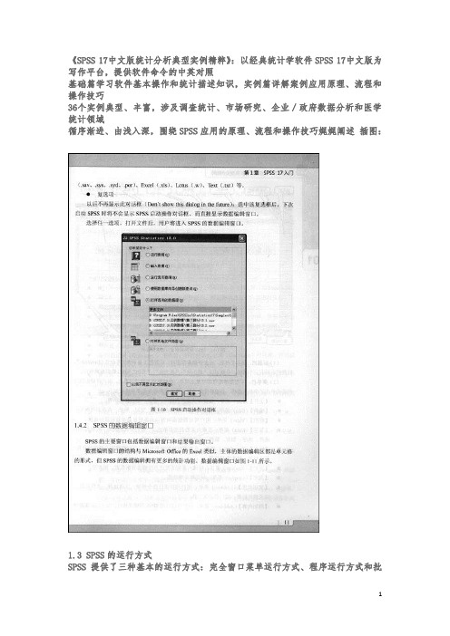
当用户运行SPSS软件后,计算机屏幕上会出现一个SPSS启动操作对话框,如图1.10所示。
在该对话框中,用户可以选择打开数据的方式。
对话框中包括一个六选一的单选按钮组和一个复选框,分别说明如下:“您希望做什么?(What would you like to do?)”单选按钮组运行教程(Runthetutorial):单击选中后,SPSS将打开帮助教程,在教程中,用户可选择不同模块的帮助说明进行有针对性的辅导。
输入数据(Type in data):需要手动输入数据,建立新的数据文件时可选择此项。
选中后,即进入空白的SPSS数据编辑窗口。
SPSS知识学习系列17.交叉表与多选题

17. 交叉表与多选题(一)基本理论分类变量包括无序分类变量、有序分类变量、多选题变量集。
对于分类变量的描述统计,主要是对分类变量各水平值分别进行频数和比例计算,再进步计算所需的一些相对频数指标。
一、单分类变量的统计描述1. 频数分布分类变量的分析,首先要了解:各类别的样本数(频数),以及占总样本量的百分比;对有序分类变量,还需要了解:累积频数、累积百分比。
2. 集中/离散趋势观察原始频数,或者使用众数。
对于分类变量,集中/离散趋势是一体的。
3. 相对频数指标(1)比(Riatio)两个有关指标之比A/B, 用来反映相对的大小关系,例如,月销售额/销售人数;(2)构成比用于描述事物内部各构成部分所占的比重,例如,百分比、累积百分比;(3)率(Rate)率是具有时间概念或速度、强度意义的指标,表示某个时期内某事件发生的频率或强度,例如速率、频率、费率、发病率等。
二、多分类变量的联合描述列联表。
例如,r×c二维列联表:(1)共n个样本;(2)按两种属性A、B,属性A有r个水平值:A1, …, A r; 属性B有c个水平值:B1, …, B c. 属性A=A i,属性B=B j的样本数为n ij.(3)n i. = “属性A=A i”的合计数,n.j = “属性B=B j”的合计数。
注:多分类变量对应高维列联表。
三、多选题的统计描述多选题是调查问卷的常见题型,因为多选题是回答同一个大问题,所以不能割裂开来单独分析,需要做汇总处理。
1. 应答人数(Count)选择各题项的人数,原始频数;2. 应答人数百分比选择该项的人数占总人数的百分比,可以反映该选项在人群中的受欢迎程度;3. 应答人次(Response)选择各选项的总人次,1个受访者选择2个选项,即2人次;4. 应答次数百分比在做出的所有选择中,选择该项的人次占总人次数的比例。
(二)SPSS实现有某调查问卷的数据文件(部分):变量属性:一、单分类变量的描述——频率变量“s4”表示学历:问题1:描述受访者的学历分布情况【分析】——【描述统计】——【频率】,将“学历”选入【变量】框,点【确定】得到S4. 学历频率百分比有效百分比累积百分比有效初中/技校或以下 154 13.4 13.4 13.4 高中/中专 313 27.3 27.3 40.7 大专331 28.9 28.9 69.6 本科 292 25.5 25.5 95.0 硕士或以上 57 5.0 5.0 100.0合计1147100.0100.0注:详细操作见第15篇《频率图表》。
spss软件练习题
spss软件练习题SPSS(Statistical Package for the Social Sciences)是一款广泛使用的统计分析软件,被广泛应用于社会科学、商业研究、医学研究等领域。
本文将为您提供SPSS软件练习题,帮助您熟悉和掌握该软件的使用。
1.数据导入与变量设置打开SPSS软件,导入名为"survey_data.sav"的数据文件。
该文件包含了一份调查问卷的数据,我们将使用这些数据进行后续的分析。
首先,通过菜单栏中的"File"→"Open"→"Data",选择并打开数据文件。
2.数据查看与描述性统计分析2.1 查看数据菜单栏的"Data"→ "View Data"可以查看数据的完整信息,包括各个变量和对应的取值。
2.2 描述性统计分析菜单栏的"Analyze"→ "Descriptive Statistics"→ "Explore"可以进行描述性统计分析,如变量的均值、标准差、最大值和最小值等。
选择需要分析的变量并点击"OK"按钮,SPSS会生成相应的结果报告。
3.数据筛选与排序3.1 数据筛选菜单栏的"Data"→"Select Cases"可以进行数据筛选,筛选出符合特定条件的数据记录。
选择"Based on conditions"并输入筛选条件,点击"OK"按钮即可得到筛选后的数据。
3.2 数据排序菜单栏的"Data"→ "Sort Cases"可以对数据进行排序,按照指定的变量进行升序或降序排序。
选择排序的变量,并设置升序或降序的方式,点击"OK"按钮即可实现排序。
2017SPSS课后作业附答案
1、习题5-4用某药治疗6位高血压病人,对每一位病人治疗前、后的舒张压进行了测量,结果如下表所示:治疗前后的舒张压测量表(2)治疗前后病人的血压是否有显著变化?将数据录入SPSS软件中,进行两配对样本T检验,分析结果如下表所示:表一统计量表二配对样本相关系数表从表一中可以看出,治疗前后高血压病人的舒张压的平均值分别为124.67、118.67,说明治疗后舒张压的平均值降低了;治疗前后这6位病人的标准分别为13.246、18.217,治疗后标准差增大了。
从表三中可以看出,治疗前后这6位病人的舒张压的差值序列的平均值为6,计算出的T统计量为1.061,其相伴概率值为0.337,比显著性水平要大,因此,不能拒绝T检验的原假设,也就是说治疗前后病人的舒张压没有显著的变化。
从两个样本平均值可以看出,治疗后的舒张压比治疗前的并没有降低很多,于是我们认为药物没有起到治疗作用。
某学校要对两位老师的教学质量进行评价,这两位老师分别教甲班和乙班,这两班数学课成绩如下表所示,这两个班的成绩是否存在差异?甲、乙两班数学考试成绩将数据录入SPSS 软件中,进行两独立样本T 检验,得到分析结果如下表所示:表一 统计量从表一中可以看出两个班数学成绩的平均值分别为83.60和75.45,对应的标准差分别为6.7、9.179,很明显甲班的数学平均成绩高于乙班。
从表二中可以得知,F 统计量的值为1.11,对应的相伴概率值为0.299,大于显著性水平0.05,不能拒绝方差相等的假设,可以认为两个老师所带的班级学生的数学成绩的方差没有显著性差异;然后观察在方差相等的条件下T 检验的结果,T 统计量的相伴概率值为0.003,小于显著性水平0.05,因此拒绝T 检验的原假设,即甲乙两班学生的数学成绩存在显著差异,从两个班数学成绩的平均值可以看出,甲班的成绩高于乙班。
甲班 90 93 82 88 85 80 87 85 74 90 88 83 82 85 73 86 77 94 68 82 乙班 76 75 73 75 98 62 90 75 83 66 65 78 80 68 87 74 64 68 72 80某职业病研究所对29名矿工中肺矽病患者、可疑患者和非患者进行了用力肺活量测定,如表6-4所示,问3组矿工的用力肺活量有无差别?用力肺活量测定数据(单位:L)肺矽病患者 1.8 1.4 1.3 1.5 1.9 1.6 1.6 1.7 2 2.1可疑患者 2.1 2.3 2.6 2.1 2.5 2.1 2.4 2.4 2.1非患者 2.8 2.9 3.2 3 3.4 3.5 3.4 2.9 3.2 3.3将数据录入SPSS软件中,进行单因素方差分析,得到分析结果如下表所示:表一方差齐性检验由上表可以看出,p值大于显著性水平0.05,因此无法拒绝方差齐性的原假设,即各个组总体方差是相等的,根据方差检验的前提条件要求,这组数据是适合进行单因素方差分析的。
spss习题及其答案
spss习题及其答案SPSS习题及其答案SPSS(Statistical Package for the Social Sciences)是一种广泛应用于社会科学研究领域的统计分析软件。
它提供了强大的数据处理和统计分析功能,使得研究人员能够更加准确地分析和解释数据。
在学习和使用SPSS的过程中,习题是一种非常有效的练习方式,能够帮助我们巩固所学知识并提高数据分析的能力。
下面将介绍几个常见的SPSS习题及其答案。
习题一:描述性统计分析某研究人员对一组学生的成绩进行了调查,并得到了以下数据:70、85、90、65、78、92、80、75、88、82。
请使用SPSS计算出这组数据的均值、标准差、最大值和最小值。
答案:打开SPSS软件,依次点击“数据”-“数据编辑器”,在变量视图中创建一个名为“成绩”的变量。
在数据视图中输入上述数据,然后点击“分析”-“描述性统计”-“描述性统计”。
将“成绩”变量移动到“变量”框中,点击“统计”按钮,在弹出的对话框中勾选“均值”、“标准差”、“最大值”和“最小值”,最后点击“确定”按钮。
SPSS将会输出这组数据的均值为80.7,标准差为8.77,最大值为92,最小值为65。
习题二:相关性分析某研究人员想要了解两个变量之间的相关性,他收集了一组学生的数学成绩和语文成绩数据。
请使用SPSS计算出这两个变量之间的相关系数。
答案:打开SPSS软件,依次点击“数据”-“数据编辑器”,在变量视图中创建两个变量分别为“数学成绩”和“语文成绩”。
在数据视图中输入相应的数据,然后点击“分析”-“相关”-“双变量”。
将“数学成绩”和“语文成绩”变量分别移动到“变量”框中,点击“确定”按钮。
SPSS将会输出这两个变量之间的相关系数,以及相关系数的显著性水平。
习题三:t检验某研究人员想要了解男性和女性在数学成绩上是否存在显著差异。
他收集了一组男性学生和一组女性学生的数学成绩数据。
请使用SPSS进行独立样本t检验。
SPSS学习系列17. 交叉表与多选题
17. 穿插表与多项选择题〔一〕根本理论分类变量包括无序分类变量、有序分类变量、多项选择题变量集。
对于分类变量的描述统计,主要是对分类变量各水平值分别进展频数和比例计算,再进步计算所需的一些相对频数指标。
一、单分类变量的统计描述1. 频数分布分类变量的分析,首先要了解:各类别的样本数〔频数〕,以及占总样本量的百分比;对有序分类变量,还需要了解:累积频数、累积百分比。
2. 集中/离散趋势观察原始频数,或者使用众数。
对于分类变量,集中/离散趋势是一体的。
3. 相对频数指标〔1〕比〔Riatio〕两个有关指标之比A/B, 用来反映相对的大小关系,例如,月销售额/销售人数;〔2〕构成比用于描述事物内部各构成局部所占的比重,例如,百分比、累积百分比;〔3〕率〔Rate〕率是具有时间概念或速度、强度意义的指标,表示某个时期内某事件发生的频率或强度,例如速率、频率、费率、发病率等。
二、多分类变量的联合描述列联表。
例如,r×c二维列联表:〔1〕共n个样本;〔2〕按两种属性A、B,属性A有r个水平值:A1, …, A r; 属性B 有c个水平值:B1, …, B c. 属性A=A i,属性B=B j的样本数为n ij.〔3〕n i. = “属性A=A i〞的合计数,n.j = “属性B=B j〞的合计数。
注:多分类变量对应高维列联表。
三、多项选择题的统计描述多项选择题是调查问卷的常见题型,因为多项选择题是答复同一个大问题,所以不能割裂开来单独分析,需要做汇总处理。
1. 应答人数〔Count〕选择各题项的人数,原始频数;2. 应答人数百分比选择该项的人数占总人数的百分比,可以反映该选项在人群中的受欢送程度;3. 应答人次〔Response〕选择各选项的总人次,1个受访者选择2个选项,即2人次;4. 应答次数百分比在做出的所有选择中,选择该项的人次占总人次数的比例。
〔二〕SPSS实现有某调查问卷的数据文件〔局部〕:变量属性:一、单分类变量的描述——频率变量“s4〞表示学历:问题1:描述受访者的学历分布情况【分析】——【描述统计】——【频率】,将“学历〞选入【变量】框,点【确定】得到S4. 学历频率百分比有效百分比累积百分比有效初中/技校或以下154 高中/中专313 大专331 本科292 硕士或以上57 合计1147注:详细操作见第15篇?频率图表?。
- 1、下载文档前请自行甄别文档内容的完整性,平台不提供额外的编辑、内容补充、找答案等附加服务。
- 2、"仅部分预览"的文档,不可在线预览部分如存在完整性等问题,可反馈申请退款(可完整预览的文档不适用该条件!)。
- 3、如文档侵犯您的权益,请联系客服反馈,我们会尽快为您处理(人工客服工作时间:9:00-18:30)。
CHAPTER 15西北研究院蔡嘉驰13124615.4 (i) What we choose is part of u t. Then gMIN t and u t are correlated, which causes OLS to be biased and inconsistent.(ii) I think it is uncorrelate because gGDP t controls for the overall performance of the U.S. economy.(iii) The change of U.S. minimum may someway change the state minimum and vice versa.If the state minimum is always the U.S. minimum, then gMIN t is exogenous in this equation and we would just use OLS.15.7 (i) Because students that would do better anyway are also more likely to attend a choice school.(ii) Since u1 does not contain income, random assignment of grants within income class means that grant designation is not correlated with unobservables such as student ability, motivation, and family support.(iii) The reduced form ischoice= π0 + π1faminc + π2grant + v2,and we need π2≠ 0.(iv) The reduced form for score is just a linear function of the exogenous variables:score= α0 + α1faminc + α2grant + v1.This equation allows us to directly estimate the effect of increasing the grant amount on the test score, holding family income fixed.So it is useful.C15.1 (i) The regression of log(wage) on sibs giveslog(wage) = 6.861 -0.0279 sibs(0.022) (0.0059)n= 935, R2= 0.023.This is a reduced form simple regression equation. It shows that, controlling for no other factors, one more sibling in the family is associated with monthly salary that is about 2.8% lower.(ii) It because older children are given priority for higher education, and families may hit budget constraints and may not be able to afford as much education for children born later. The simple regression of educ on brthord giveseduc = 14.15 - 0.283 brthord(0.13) (0.046)n= 852, R2= 0.042.The equation predicts that every one-unit increase in brthord reduces predicted education by about 0.28 years.(iii) When brthord is used as an IV for educ in the simple wage equation we getlog(wage) = 5.03 + 0.131 educ(0.42) (0.031)n= 852.Because of missing data on brthord, we are using fewer observations than in the previous analyses.(iv) In the reduced form equationeduc= π0 + π1sibs + π2brthord + v,we need π2≠ 0 in order for the βj to be identified. We take the null to be H0: π2 = 0, and look to reject H0 at a small significance level.ˆπ = The regression of educ on sibs and brthord (using 852 observations) yields2ˆπ) = 0.057. The p is about 0.000, which rejects H0 fairly strongly. -0.153 and se(2Therefore, the identification assumptions appears to hold.(v) The equation estimated by IV islog(wage) = 4.94 + 0.137 educ+ 0.0021 sibs(1.06) (0.075) (0.0174)n= 852.βis much larger than we obtained in part (iii). The 95% The standard error on ˆeducβis roughly -.010 to .284, which is very wide and includes the value zero. CI foreducβis very large, rendering sibs very insignificant.The p of ˆsibs(vi)the correlation between educ i and sibs i is about -0.930, which is a very strong negative correlation. This means that, for the purposes of using IV, multicollinearity is a serious problem here, and is not allowing us to estimate βeduc with much precision. C15.2 (i) The equation estimated by OLS ischildren = -4.138 -0.0906 educ+ 0.332 age-0.00263 age2(0.241) (0.0059) (0.017) (0.00027)n= 4.361, R2= 0.569.Another year of education, holding age fixed, results in about 0.091 fewer children.In other words, for a group of 100 women, if each gets another of education, they collectively are predicted to have about nine fewer children.(ii) The reduced form for educ iseduc= π0 + π1age + π2age2 + π3frsthalf + v,and we need π3≠ 0.When we run the regression we obtain 3ˆπ= -0.852 and se(3ˆπ) = 0.113. Therefore, women born in the first half of the year are predicted to have almost one year lesseducation, holding age fixed. The p on frsthalf is 0 and so the identification condition holds.(iii) The structural equation estimated by IV ischildren = -3.388 - 0.1715 educ + 0.324 age - 0.00267 age 2(0.548) (0.0532) (0.018) (0.00028)n = 4.361, R 2 = 0.550.The estimated effect of education on fertility is now much larger. Naturally, the standard error for the IV estimate is also bigger, about nine times bigger.(iv) When we add electric, tv, and bicycle to the equation and estimate it by OLS we obtainchildren = -4.390 - .0767 educ+ 0.340 age-0.00271 age2-0.303 electric(0.0240) (0.0064) (0.016) (0.00027) (0.076)-0.253 tv +0.318 bicycle(0.091) (0.049)n= 4,356, R2= 0.576.The 2SLS (or IV) estimates arechildren = -3.591 -0.1640 educ + 0.328 age-0.00272 age2-0.107 electric(0.645) (0.0655) (0.019) (0.00028) (0.166)-0.0026 tv+ 0.332 bicycle(0.2092) (0.052)n= 4,356, R2= 0.558.Adding electric, tv, and bicycle to the model reduces the estimated effect of educ in both cases, but not by too much. In the equation estimated by OLS, the coefficient on tv implies that, other factors fixed, four families that own a television will have about one fewer child than four families without a TV. Television ownership can be a proxy for different things, including income and perhaps geographic location. A causal interpretation is that TV provides an alternative form of recreation.Interestingly, the effect of TV ownership is practically and statistically insignificant in the equation estimated by IV. The coefficient on electric is also greatly reduced in magnitude in the IV estimation. The substantial drops in the magnitudes of these coefficients suggest that a linear model might not be the best functional form, which would not be surprising since children is a count variable.CHAPTER 16西北研究院蔡嘉驰13124616.1 (i) If α1 = 0 then y1 = β1z1 + u1, and so it depends only on the exogenous variable z1 and the error term u1. This then is the reduced form for y1. If α1 = 0, the reduced form for y1 is y1 = β2z2 + u2.If α1≠ 0 and α2 = 0:β2z2 + u2= α1y2 + β1z1 + u1Dividing by α1 givesy2= (β1/α1)z1– (β2/α1)z2 + (u1–u2)/α1≡π21z1 + π22z2 + v2,where π21 = β1/α1, π22 = -β2/α1, and v2 = (u1–u2)/α1.(ii) y1– (α1/α2)y1= α1y2-α1y2 + β1z1– (α1/α2)β2z2 + u1– (α1/α2)u2= β1z1– (α1/α2)β2z2 + u1– (α1/α2)u2Because α1≠α2, 1 – (α1/α2) ≠ 0, and so we can obtain the reduced form for y1:y1 = π11z1 + π12z2 + v1,where π11 = β1/[1 – (α1/α2)], π12 = -(α1/α2)β2/[1 – (α1/α2)],and v1 = [u1– (α1/α2)u2]/[1 – (α1/α2)].A reduced form does exist for y2, as can be seen by subtracting the second equation from the first:0 = (α1–α2)y2 + β1z1–β2z2 + u1–u2;because α1≠α2, we can rearrange and divide by α1-α2 to obtain the reduced form.(iii) In supply and demand examples, α1≠α2 is very reasonable. If the first equation is the supply function, we generally expect α1 > 0, and if the second equation is the demand function, α2 < 0.16.2the first equation must be the demand function, as it depends on income, which is a common determinant of demand.The second equation contains a variable, rainfall, that affects crop production and therefore corn supply.C16.3 (i) The OLS estimates areinf = 25.23 - 0.215 open(4.10) (0.093)n= 114, R2= 0.045.The IV estimates areinf = 29.57 - 0.332 open(5.65) (0.140)n= 114, R2= 0.032.The OLS coefficient is the same, to three decimal places, when log(pcinc) is included in the model.The IV estimate with log(pcinc) in the equation is -0.337, which is very close to-0.333.Therefore, dropping log(pcinc) makes little difference.(ii) If we regress open on land we obtain R2 = .095.The simple regression of open on log(land) gives R2 = .448.Therefore, log(land) is much more highly correlated with open. Further, if we regress open on log(land) and land we getopen = 129.22 8.40 log(land) + 0.0000043 land(10.47) (0.98) (0.0000031)n= 114, R2= 0.457.While log(land) is very significant, land is not, so we might as well use only log(land) as the IV for open.(iii) When we add oil to the original model, and assume oil is exogenous, the IV estimates areinf = 24.01 -0.337 open+ 0.803 log(pcinc) - 6.56 oil(16.04) (0.144) (2.12) (9.80)n= 114, R2= .035.Being an oil producer is estimated to reduce average annual inflation by over 6.5 percentage points, but the effect is not statistically significant because p=0.505C16.8(i) To estimate the demand equations, we need at least one exogenous variable that appears in the supply equation.(ii) For wave2t and wave3t to be valid IVs for log(avgprc t), we need two assumptions.The first is that these can be properly excluded from the demand equation. The second assumption is that at least one of wave2t and wave3t appears in the supply equation. There is indirect evidence of this in part three, as the two variables are jointly significant in the reduced form for log(avgprc t).(iii) The OLS estimates of the reduced form arelog(avgprc) =-1.02 - 0.012 mon t- 0.0090 tues t + 0.051 wed t+ 0.124 thurs t(0.14) (0.114) (0.1119) (0.112) (0.111)+ 0.094 wave2t+ 0.053 wave3t(0.021) (0.020)n = 97, R2 = 0.304The variables wave2t and wave3t are jointly very significant: F = 19.1, p-value = zero to four decimal places.(iv) The 2SLS estimates of the demand function arelog(totqty) =8.16 - 0.816 log(avgprc t) -0.307 mon t- 0.685 tues t(0.18) (0.327) (0.229) (0.226)-0.521 wed t+ 0.095 thurs t(0.224) (0.225)n = 97, R2 = 0.193The 95% confidence interval for the demand elasticity is roughly -1.47 to -0.17. The point estimate, -0.82, seems reasonable: a 10 percent increase in price reduces quantity demanded by about 8.2%.(v)The coefficient on ,1ˆi t u- is about-1.33 (se =0.593), so there is strong evidence of negative serial correlation, although the estimate of ρ is not huge.(vi) To estimate the supply elasticity, we would have to assume that theday-of-the-week dummies do not appear in the supply equation, but they do appear in the demand equation.(vii) Unfortunately, in the estimation of the reduced form for log(avgprc t ) in part (iii), the variables mon , tues , wed , and thurs are jointly insignificant [F (4,90) = 0.53, p -value = 0.71.]This means that, while some of these dummies seem to show up in the demand equation, things cancel out in a way that they do not affect equilibrium price, once wave2 and wave3 are in the equation.CHAPTER 17西北研究院 蔡嘉驰 13124617.2We need to compute the estimated probability first at hsGPA = 3.0, SAT = 1,200, and study = 10 and subtract this from the estimated probability with hsGPA = 3.0, SAT = 1,200, and study = 5.we start by computing the linear function inside Λ(⋅): -1.77 + 0.24(3.0) +0.00058(1,200) + 0.073(10) = 0.376.Next, we plug this into the logit function: exp(0.376)/[1 + exp(0.376)] ≈ 0.593. For the student-athlete who attended study hall five hours a week, we compute –1.77 + 0.24(3.0) +0 .00058(1,200) + 0.073(5) =0 .011. Evaluating the logit function at this value gives exp(0.011)/[1 + exp(0.011)] ≈ 0.503. Therefore, the difference in estimated probabilities is 0.593 - 0.503 = 0.090, or just under 0.10. 17.5(i) patents is a count variable, and so the Poisson regression model is appropriate.(ii) Because β1 is the coefficient on log(sales ), β1 is the elasticity of patents with respect to sales .(iii) We use the chain rule to obtain the partial derivative of exp[β0 +β1log(sales ) + β2RD + β3RD 2] with respect to RD :(|,)E patents sales RD RD∂∂ = (β2 + 2β3RD )exp[β0 + β1log(sales ) + β2RD + β3RD 2]. A simpler way to interpret this model is to take the log and then differentiate with respect to RD : this gives β2 + 2β3RD , which shows that the semi-elasticity of patents with respect to RD is 100(β2 + 2β3RD ).C17.3(i)Out of 616 workers, 172, or about 18%, have zero pension benefits.For the 444 workers reporting positive pension benefits, the range is from $7.28 to $2,880.27.Therefore, we have a nontrivial fraction of the sample with pension t = 0, and the range of positive pension benefits is fairly wide. The Tobit model is well-suited to this kind of dependent variable.(ii) The Tobit results are given in the following table:In column (1), which does not control for union, being white or male (or, of course, both) increases predicted pension benefits, although only male is statistically significant (t≈ 4.41).(iii) We use equation (17.22) with exper = tenure = 10, age = 35, educ = 16, depends = 0, married = 0, white = 1, and male = 1 to estimate the expected benefit for a white male with the given characteristics.ˆxβ= -1,252.5+5.20(10)–4.64(35) +36.02(10)+93.21(16) + 144.09 + 308.15 = 940.90. Therefore, with ˆσ = 677.74 we estimate E(pension|x) asΦ(940.9/677.74)⋅(940.9) + (677.74)⋅φ(940.9/677.74) ≈966.40.For a nonwhite female with the same characteristics,ˆxβ= -1,252.5 + 5.20(10) – 4.64(35) + 36.02(10) + 93.21(16) = 488.66. Therefore, her predicted pension benefit isΦ(488.66/677.74)⋅(488.66) + (677.74)⋅φ(488.66/677.74) ≈582.10.The difference between the white male and nonwhite female is966.40 – 582.10 = $384.30.(iv) Column (2) in the previous table gives the results with union added. The coefficient is large, but to see exactly how large, The t statistic on union is over seven.(v)When peratio is used as the dependent variable in the Tobit model, white and male are individually and jointly insignificant.C17.5 (i) The Poisson regression results are given in the following table:The coefficient on y82means that, other factors in the model fixed, a woman’s fertility was about 19.3% lower in 1982 than in 1972.(ii) Because the coefficient on black is so large, we obtain the estimated proportionate difference as exp(0.36) – 1 ≈0.433, so a black woman has 43.3% more children than a comparable nonblack woman.(iii)From the above table, ˆσ = 0.996, which shows that there is actually underdispersion in the estimated model.(iv) The sample correlation is about 0.348, which means the R-squared is about (0.348)2 0.121.Interestingly, this is actually smaller than the R-squared for the linear model estimated by OLS.。