Performing Fourier Transforms in Mathematica

Justin Young

young.1022@https://www.360docs.net/doc/1c9249320.html,

The Ohio State University

Department of Physics Performing Fourier Transforms in Mathematica

Mathematica is one of many numerical software packages that offers support for Fast Fourier Transform algorithms. You can perform manipulations with discrete data that you have collected in the laboratory, as well as with continuous, analytical functions. This tutorial introduces some of the common functions used to perform these calculations as well as some basic concepts and caveats that are specific to Mathematica.

Load data file into an array

It is often the case that you have a text file that contains a number of discrete data points that you have collected and need to analyze. This data file may be a comma-, space-, or tab- delimited

(.csv) file, text file (.txt), or any other file supported by Mathematica. (Run the "$ImportFormats" command to see all supported data types.) In this tutorial, we will use the "Import" command to import an existing text file that contains some electric field data into an array (Mathematica calls arrays 'lists'). You will need to specify the path to your data file.

Important! If your data is in a non-standard format, you might need to modify the way this notebook imports your data. The if statement below checks how the data file is structured and modifies the array appropriately in order for the rest of this notebook to work. This code assumes you have a data file with a separate row for each data point. It can handle data points specified as real field values at each time, in two columns, as well as data that has been separated into real and imaginary components at each time, in three columns. If your data file is structured differently, you will have to modify how the data arrays are being referenced throughout the rest of the notebook. This is not difficult--if you have an array called myArray, Mathematica references elements of the array as myArray[[4]], for the 4th entry, for example (it does NOT use a 0-based index). For multi-dimensional arrays, you can reference elements using myArray[[4]][[2]], in order to get the 2nd element of the 4th element of the array, for example.

data Import "sample.txt","Table" ;

n Length data ;

If Length data 1 3,

data Table data i 1 ,data i 2 data i 3 , i,1,n ;

Plot the waveform in the time domain

It is useful to plot the data both to get an idea of what it looks like in the time domain and to make sure it loaded properly.

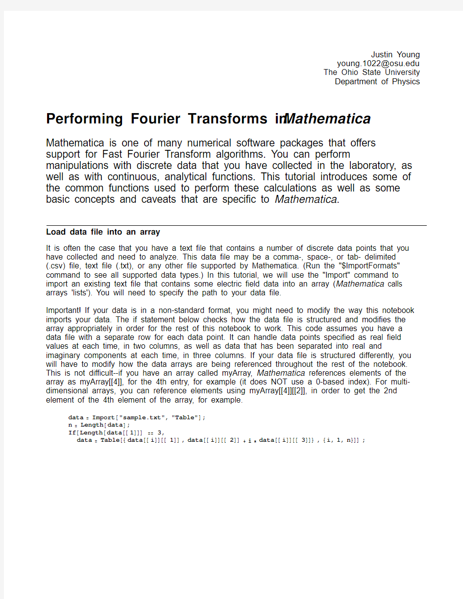
Plot the real part of the electric field E(t) by providing an array of (t,Re(E(t))) data points and passing it to the ListPlot function. The array is created using the Table function. (If you are familar with basic programming structures, Table is essentially a 'for' loop.)

In[139]:=ListPlot Table data i 1 ,Re data i 2 , i,1,n ,

Joined True,PlotRange All,FrameLabel "t","Re E t " ,Frame True

Out[139]= 10 50

510 0.2

0.0

0.2

0.4

0.6

0.8

1.0

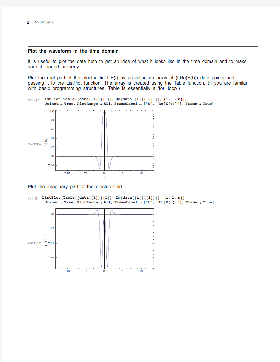
t R e E t Plot the imaginary part of the electric field.

In[140]:=ListPlot Table data i 1 ,Im data i 2 , i,1,n ,

Joined True,PlotRange All,FrameLabel "t","Im E t " ,Frame True

Out[140]= 10 50

510

0.6

0.4

0.2

0.0

t I m E t 2 MyTutorial.nb

Plot the intensity of the field.

In[141]:=ListPlot Table data i 1 ,Abs data i 2 2 , i,1,n ,

Joined True,PlotRange All,FrameLabel "t","Intensity" ,Frame True

Out[141]= 10 50

5100.0

0.2

0.4

0.6

0.81.0

t I n t e n s i t y Transform the data into the frequency domain

Find the temporal spacing between data points. In this example, the spacing is the same between all the data points.

In[142]:=

t data 2 1 data 1 1 Out[142]=0.1

Create an array of the field amplitudes to pass to the Fourier function.

In[143]:=fieldValues Table data i 2 , i,1,n ;

Compute the Fourier transform E(?) using the built-in function. Important! The sample data array is ordered from negative times to positive times. However, Mathematica requires that the array

passed to the Fourier function be ordered starting with the t=0 element, ascending to positive time elements, then negative time elements. To account for this, we run the RotateLeft command on our data array. The array that results after taking the transform is ordered starting from zero-frequency, increasing to the maximum frequency; then it jumps to the most negative frequency, and increases to zero. Therefore, when we want to plot the result of the transform in frequency space, we need to shift the array again after the transform. We use RotateRight (by the same amount) before plotting, so that our data is ordered from negative frequencies to positive frequencies, with the zero frequency component in the middle.

In[144]:=FFTValues Fourier RotateLeft fieldValues,n 2 1 ,FourierParameters 1, 1 ;

FFTValues RotateRight FFTValues,n 2 1 ;

Find the spectral spacing (in Hz).

In[146]:=

Ν 1n t Out[146]=0.0390625

a list of frequency-axis values (in angular Hz) to use in the plot of E(?).

MyTutorial.nb 3

Create a list of frequency-axis values (in angular Hz) to use in the plot of E(?).

In[147]:=frequencyValues Table Ν i n 2 , i,1,n ;Plot the waveform in the frequency domain

Plot the real part of E(Ν).

In[148]:=ListPlot Table frequencyValues i ,Re FFTValues i , i,1,n ,

Joined True,PlotRange All,FrameLabel "Ν","Re E Ν " ,Frame True

Out[148]= 4 20

ΝR e E Ν

Plot the imaginary part.

In[149]:=ListPlot Table frequencyValues i ,Im FFTValues i , i,1,n ,

Joined True,PlotRange All,FrameLabel "Ν","Im E Ν " ,Frame True

Out[149]= 4 20

ΝI m E Ν 4 MyTutorial.nb

Plot the frequency power intensity spectrum.

In[150]:=ListPlot Table frequencyValues i ,Abs FFTValues i 2 , i,1,n ,

PlotRange All,Joined True,FrameLabel "Ν","Intensity" ,Frame True

Out[150]= 4 20

100150

200

ΝI n t e n s i t y Plot the spectral phase of the waveform versus frequency

Since complex values have an associated phase in the complex plane, we want to plot the spectral phase as a function of frequency. However, the Arg(z) function is periodic in multiples of 2Π. Therefore, we need to 'unwrap' the angles. Unfortunately, Mathematica does not provide a built-in function to do this. Here is some short code that provides this functionality, returns the phase values in an array, and plots the values.

In[151]:=phase Arg FFTValues ;

phase FoldList Round 1 2 2Pi 2Pi 2&,First phase ,Rest phase ;

ListPlot Table frequencyValues i ,phase i , i,1,n ,

Joined True,PlotRange All,FrameLabel "Ν","Φ" ,Frame True

Out[153]= 4 20

ΝΦ

MyTutorial.nb 5

Inverse transform back into the time domain

Perform a reverse Fourier transform (remembering to shift the array before the transform, since we plotted it above ordered from negative to positive values!).

In[154]:=originalFFTValues

InverseFourier RotateLeft FFTValues,n 2 1 ,FourierParameters 1, 1 ;

Plot the intensity versus time (remembering to shift the array before plotting...you should be good at this by now)

In[155]:=originalPulse RotateRight originalFFTValues,n 2 1 ;

ListPlot Table data i 1 ,Abs originalPulse i 2 , i,1,n ,

Joined True,PlotRange All,FrameLabel "t","Intensity" ,Frame True

Out[156]= 10 50

5100.00.20.40.60.81.0

t I n t e n s i t y As expected, we get the same pulse back as before, since we did not apply any transfer function to it in the frequency domain. This is a good test to see if your software is working.

Working with analytic functions

You can take the Fourier transform of an analytic function as follows ...

In[157]:=FourierTransform Exp a t 2 ,t,?,FourierParameters 1, 1

Out[157]=

4a Π

a ... as well as its inverse

In[158]:=InverseFourierTransform

Πa ,?,t,FourierParameters 1, 1

Out[158]=

a t 2 can use these methods to create discrete data sets from a given analytic expression, for example, by sampling at specified times and frequencies.

6 MyTutorial.nb

MyTutorial.nb7

You can use these methods to create discrete data sets from a given analytic expression, for example, by sampling at specified times and frequencies.

Possible Issues

Here are some common issues you might run into when using Mathematica, as well as general things to keep in mind when performing Fourier transforms.

When working with analytic functions, be aware of the sign convention used for plane waves traveling to the left and those traveling to the right.

You are free to choose the sign convention you prefer when distinguishing between forward and reverse transforms, as long as you are consistent. Mathematica' s convention is different from that used in class, but you can force Mathematica to use a specified convention by setting the FourierParameters property in the Fourier and InverseFourier functions. I have set my transforms to use the sign convention used in class. See the documentation for more information.

When generating sample data to work with, make sure your sample window is large enough in order to accomodate the entire signal of interest. This may involve using more or less data points, or setting different temporal and spectral spacings.

It is easy to get the array rotations mixed up when preparing your array for forward and reverse transforms, and in plotting. However, it is easy to tell if your array ordering is incorrect; your data will appear to be discontinuous. Perform another rotation and try plotting it again.

In order to avoid array rotation problems when you make a change in your notebook, such as in a transfer function, it is useful to re-evaluate the entire notebook from start to end in order to properly reset your arrays.

Make sure you are using frequency values or angular frequency values, as appropriate.

It is often convenient to work only with the pulse envelope. Therefore, be sure to distinguish between instantaneous and carrier frequencies in your calculations.

Check the scale of your units to be sure everything matches up! (e.g. Hz vs. THz)

Summary

With these tools, you should now be able to perform forward and reverse Fourier transforms of discrete and continuous data sets in Mathematica. You have seen that the Table function is one of the most useful functions in Mathematica to create and manipulate arrays. You have also seen some of the ways that you can visualize your data, by way of examining the magnitudes and phases of complex-valued fields, as well as their frequency spectra. The best way to learn about Mathematica's capabilities is to simply start using the software and try as many examples as possible. The documentation is quite helpful when you need a description of what certain functions do, what their assumptions are, and what parameters they can take. Most manual pages give you examples to work with that you can modify for your own purposes. The web is also a great resource for finding examples. Have fun transfoming, please email me if you find any errors in this document, and remember, transforms are just robots in disguise!