MATLAB实验报告实例
Matlab实验报告
实验一:Matlab操作环境熟悉一、实验目的1.初步了解Matlab操作环境。
2.学习使用图形函数计算器命令funtool及其环境。
二、实验内容熟悉Matlab操作环境,认识命令窗口、内存工作区窗口、历史命令窗口;学会使用format命令调整命令窗口的数据显示格式;学会使用变量和矩阵的输入,并进行简单的计算;学会使用who和whos命令查看内存变量信息;学会使用图形函数计算器funtool,并进行下列计算:1.单函数运算操作。
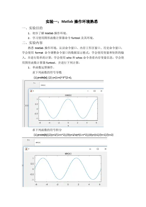
求下列函数的符号导数(1)y=sin(x); (2) y=(1+x)^3*(2-x);求下列函数的符号积分(1)y=cos(x);(2)y=1/(1+x^2);(3)y=1/sqrt(1-x^2);(4)y=(x1)/(x+1)/(x+2)求反函数(1)y=(x-1)/(2*x+3); (2) y=exp(x); (3) y=log(x+sqrt(1+x^2));代数式的化简(1)(x+1)*(x-1)*(x-2)/(x-3)/(x-4);(2)sin(x)^2+cos(x)^2;(3)x+sin(x)+2*x-3*cos(x)+4*x*sin(x);2.函数与参数的运算操作。
从y=x^2通过参数的选择去观察下列函数的图形变化(1)y1=(x+1)^2(2) y2=(x+2)^2(3) y3=2*x^2 (4) y4=x^2+2 (5) y5=x^4 (6)y6=x^2/23.两个函数之间的操作求和(1)sin(x)+cos(x) (2) 1+x+x^2+x^3+x^4+x^5乘积(1)exp(-x)*sin(x) (2) sin(x)*x商(1)sin(x)/cos(x); (2) x/(1+x^2); (3) 1/(x-1)/(x-2);求复合函数(1)y=exp(u) u=sin(x) (2) y=sqrt(u) u=1+exp(x^2)(3) y=sin(u) u=asin(x) (4) y=sinh(u) u=-x实验二:MATLAB基本操作与用法一、实验目的1.掌握用MATLAB命令窗口进行简单数学运算。
MATLAB实验报告实例

MATLAB课程设计院(系)数学与计算机学院专业信息与计算科学班级学生姓名学号指导老师赵军产提交日期实验内容: 1. Taylor逼近的直观演示用Taylor 多项式逼近y = sin x.已知正弦函数的Taylor 逼近式为∑=----=≈nkk kkxxPx1121!)12()1()(sin.实验目的:利用Taylor多项式逼近y = sin x,并用图形直观的演示。
实验结果报告(含基本步骤、主要程序清单、运行结果及异常情况记录等):1.将k从1取到5,得到相应的P = x-1/6*x^3+1/120*x^5-1/5040*x^7+1/362880*x^9;2.用MATLAB进行Taylor逼近,取x的范围是(-3.2,3.2);程序清单如下:syms x; y = sin(x); p = x - (x^3)/6 + (x^5)/120 - (x^7)/5040 + (x^9)/362880 x1 = -3.2:0.01:3.2;ya = sin(x1);y1 = subs(p,x,x1);plot(x1,ya,'-',x1,y1)4.程序运行正常。
思考与深入:取y = sin x 的Taylor 多项式为P 的逼近效果很良好,基本接近y = sin x 的图像,不过随着k 的取值变多,逼近的效果会越来越好。
实验内容: 2. 数据插值在(,)[8,8][8,8]x y =-⨯-区域内绘制下面曲面的图形:2222sin()x y z x y+=+并比较线性、立方及样条插值的结果。
.实验目的:学会用MATLAB对函数进行线性、立方及样条插值,并比较结果。
实验结果报告(含基本步骤、主要程序清单、运行结果及异常情况记录等):1.用MATLAB一次进行对函数的线性、立方、及样条插值,并进行算法误差分析。
2.主要程序如下:[x,y] = meshgrid(-8:1:8,-8:1:8);z = sin((x.^2 + y.^2).^0.5)./((x.^2 + y.^2).^0.5);surf(x,y,z),axis([-8,8,-8,8,-2,3])title('z的曲面图形'); %画出z的曲面图形%选较密的插值点,用默认的线性插值算法进行插值figure;[x1,y1] = meshgrid(-8:0.4:8,-8:0.4:8);z1=interp2(x,y,z,x1,y1);surf(x1,y1,z1),axis([-8,8,-8,8,-2,3])title('线性插值');%立方和样条插值figure;z1=interp2(x,y,z,x1,y1,'cubic');z2=interp2(x,y,z,x1,y1,'spline');surf(x1,y1,z1),axis([-8,8,-8,8,-2,3])title('立方插值');figure;surf(x1,y1,z2),axis([-8,8,-8,8,-2,3])title('样条插值');%算法误差的比较z = sin((x1.^2 + y1.^2).^0.5)./((x1.^2 + y1.^2).^0.5);figure;title('误差分析1');figure;surf(x1,y1,abs(z-z2)),axis([-8,8,-8,8,0,0.025]) title('误差分析2');3.结果如下:4.程序运行正常。
MATLAB信号与系统实验报告19472[五篇范文]
![MATLAB信号与系统实验报告19472[五篇范文]](https://uimg.taocdn.com/a72999dee109581b6bd97f19227916888486b9f2.webp)
MATLAB信号与系统实验报告19472[五篇范文]第一篇:MATLAB信号与系统实验报告19472信号与系统实验陈诉(5)MATLAB 综合实验项目二连续系统的频域阐发目的:周期信号输入连续系统的响应可用傅里叶级数阐发。
由于盘算历程啰嗦,最适适用MATLAB 盘算。
通过编程实现对输入信号、输出信号的频谱和时域响应的盘算,认识盘算机在系统阐发中的作用。
任务:线性连续系统的系统函数为11)(+=ωωjj H,输入信号为周期矩形波如图 1 所示,用MATLAB 阐发系统的输入频谱、输出频谱以及系统的时域响应。
-3-2-1 0 1 2 300.511.52Time(sec)图 1要领:1、确定周期信号 f(t)的频谱nF&。
基波频率Ω。
2、确定系统函数 )(Ω jn H。
3、盘算输出信号的频谱n nF jn H Y&&)(Ω=4、系统的时域响应∑∞-∞=Ω=nt jnn eY t y&)(MATLAB 盘算为y=Y_n*exp(j*w0*n“*t);要求(画出 3 幅图):1、在一幅图中画输入信号f(t)和输入信号幅度频谱|F(jω)|。
用两个子图画出。
2、画出系统函数的幅度频谱|H(jω)|。
3、在一幅图中画输出信号y(t)和输出信号幅度频谱|Y(jω)|。
用两个子图画出。
解:(1)阐发盘算:输入信号的频谱为(n)输入信号最小周期为=2,脉冲宽度,基波频率Ω=2π/ =π,所以(n)系统函数为因此输出信号的频谱为系统响应为(2)步伐:t=linspace(-3,3,300);tau_T=1/4;%n0=-20;n1=20;n=n0:n1;%盘算谐波次数20F_n=tau_T*Sa(tau_T*pi*n);f=2*(rectpuls(t+1.75,0.5)+rectpuls(t-0.25,0.5)+rectpuls(t-2.25,0.5));figure(1),subplot(2,1,1),line(t,f,”linewidth“,2);%输入信号的波形 axis([-3,3,-0.1,2.1]);grid onxlabel(”Time(sec)“,”fontsize“,8),title(”输入信号“,”fontweight“,”bold“)%设定字体巨细,文本字符的粗细text(-0.4,0.8,”f(t)“)subplot(2,1,2),stem(n,abs(F_n),”.“);%输入信号的幅度频谱xlabel(”n“,”fontsize“,8),title(”输入信号的幅度频谱“,”fontweight“,”bold“)text(-4.0,0.2,”|Fn|“)H_n=1./(i*n*pi+1);figure(2),stem(n,abs(H_n),”.“);%系统函数的幅度频谱xlabel(”n“,”fontsize“,8),title(”系统函数的幅度频谱“,”fontweight“,”bold“)text(-2.5,0.5,”|Hn|“)Y_n=H_n.*F_n;y=Y_n*exp(i*pi*n”*t);figure(3),subplot(2,1,1),line(t,y,“linewidth”,2);%输出信号的波形 axis([-3,3,0,0.5]);grid onxlabel(“Time(sec)”,“fontsize”,8),title(“输出信号”,“fontweight”,“bold”)text(-0.4,0.3,“y(t)”)subplot(2,1,2),stem(n,abs(Y_n),“.”);%输出信号的幅度频谱xlabel(“n”,“fontsize”,8),title(“输出信号的幅度频谱”,“fontweight”,“bold”)text(-4.0,0.2,“|Yn|”)(3)波形:-3-2-1 0 1 2 300.511.52Time(sec)输入信号f(t)-20-15-10-5 0 5 10 15 2000.10.20.30.4n输入信号的幅度频谱|Fn|-20-15-10-5 0 5 10 15 2000.10.20.30.40.50.60.70.80.91n系统函数的幅度频谱|Hn|-3-2-1 0 1 2 300.10.20.30.4Time(sec)输出信号y(t)-20-15-10-5 0 5 10 15 2000.10.20.30.4n输出信号的幅度频谱|Yn| 项目三连续系统的复频域阐发目的:周期信号输入连续系统的响应也可用拉氏变更阐发。
程序设计实验报告(matlab)

程序设计实验报告(matlab)实验一: 程序设计基础实验目的:初步掌握机器人编程语言Matlab。
实验内容:运用Matlab进行简单的程序设计。
实验方法:基于Matlab环境下的简单程序设计。
实验结果:成功掌握简单的程序设计和Matlab基本编程语法。
实验二:多项式拟合与插值实验目的:学习多项式拟合和插值的方法,并能进行相关计算。
实验内容:在Matlab环境下进行多项式拟合和插值的计算。
实验方法:结合Matlab的插值工具箱,进行相关的计算。
实验结果:深入理解多项式拟合和插值的实现原理,成功掌握Matlab的插值工具箱。
实验三:最小二乘法实验目的:了解最小二乘法的基本原理和算法,并能够通过Matlab进行计算。
实验内容:利用Matlab进行最小二乘法计算。
实验方法:基于Matlab的线性代数计算库,进行最小二乘法的计算。
实验结果:成功掌握最小二乘法的计算方法,并了解其在实际应用中的作用。
实验六:常微分方程实验目的:了解ODE的基本概念和解法,并通过Matlab进行计算。
实验内容:利用Matlab求解ODE的一阶微分方程组、变系数ODE、高阶ODE等问题。
实验方法:基于Matlab的ODE工具箱,进行ODE求解。
实验结果:深入理解ODE的基本概念和解法,掌握多种ODE求解方法,熟练掌握Matlab的ODE求解工具箱的使用方法。
总结在Matlab环境下进行程序设计实验,使我对Matlab有了更深刻的认识和了解,也使我对计算机科学在实践中的应用有了更加深入的了解。
通过这些实验的学习,我能够灵活应用Matlab进行各种计算和数值分析,同时也能够深入理解相关的数学原理和算法。
这些知识和技能对我未来的学习和工作都将有着重要的帮助。
matlab实验报告
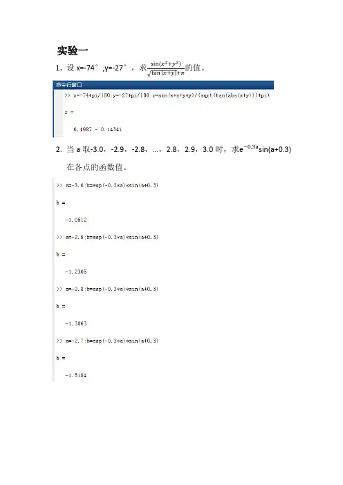
实验一1.设x=-74°,y=-27°,求22的值。
√tan|x+y|+π2.当a取-3.0,-2.9,-2.8,…,2.8,2.9,3.0时,求e−0.3a sin(a+0.3)在各点的函数值。
3. 设x=24−0.455,求12In(x+√1+x ²)的值,并分析结果矩阵中各元素的含义。
4. 已知A=354234−457879015,B=1−2672874930求下面的表达式的值。
(1)A*B和A.*B。
(2)A^3和A.^3.。
(3)A/B和A\B。
(4)[A,B]和[A([1,3],:);B^2]。
实验二一、实验步骤:1)新建脚本2)在编辑器中输入相应程序3)在命令窗口执行文件,得到结果1. 根据π²6=11²+12²+13²+…+1n ²,求π的近似值。
当n 分别取100、1000、10000时,结果是多少?要求:分别用循环结构和向量运算(使用sum 函数)来实现。
1)循环结构一、实验步骤二、1)新建脚本2)在编辑器中输入相应程序3)保存文件,将文件命名为PI.m4)在命令窗口输入PI执行文件,得到结果三、实验代码四、实验结果2.根据y=1+13+15+⋯+12n−1,求(1)y<3时的最大n值(2)与(1)的n值对应的y值一、实验步骤1)打开matlab,新建脚本2)在脚本文件中输入实验代码3)保存文件,存名字为value.m4)在命令窗口中输入value,得到实验结果二、实验代码三、实验结果。
MATLAB实验报告(1-4)
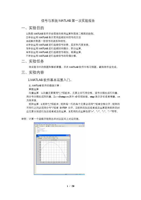
信号与系统MATLAB第一次实验报告一、实验目的1.熟悉MATLAB软件并会简单的使用运算和简单二维图的绘制。
2.学会运用MATLAB表示常用连续时间信号的方法3.观察并熟悉一些信号的波形和特性。
4.学会运用MATLAB进行连续信号时移、反折和尺度变换。
5.学会运用MATLAB进行连续时间微分、积分运算。
6.学会运用MATLAB进行连续信号相加、相乘运算。
7.学会运用MATLAB进行连续信号的奇偶分解。
二、实验任务将实验书中的例题和解析看懂,并在MATLAB软件中练习例题,最终将作业完成。
三、实验内容1.MATLAB软件基本运算入门。
1). MATLAB软件的数值计算:算数运算向量运算:1.向量元素要用”[ ]”括起来,元素之间可用空格、逗号分隔生成行向量,用分号分隔生成列向量。
2.x=x0:step:xn.其中x0位初始值,step表示步长或者增量,xn为结束值。
矩阵运算:1.矩阵”[ ]”括起来;矩阵每一行的各个元素必须用”,”或者空格分开;矩阵的不同行之间必须用分号”;”或者ENTER分开。
2.矩阵的加法或者减法运算是将矩阵的对应元素分别进行加法或者减法的运算。
3.常用的点运算包括”.*”、”./”、”.\”、”.^”等等。
举例:计算一个函数并绘制出在对应区间上对应的值。
2).MATLAB软件的符号运算:定义符号变量的语句格式为”syms 变量名”2.MATLAB软件简单二维图形绘制1).函数y=f(x)关于变量x的曲线绘制用语:>>plot(x,y)2).输出多个图像表顺序:例如m和n表示在一个窗口中显示m行n列个图像,p表示第p个区域,表达为subplot(mnp)或者subplot(m,n,p)3).表示输出表格横轴纵轴表达范围:axis([xmax,xmin,ymax,ymin])4).标上横轴纵轴的字母:xlabel(‘x’),ylabel(‘y’)5).命名图像就在subplot写在同一行或者在下一个subplot前:title(‘……’)6).输出:grid on举例1:举例2:3.matlab程序流程控制1).for循环:for循环变量=初值:增量:终值循环体End2).while循环结构:while 逻辑表达式循环体End3).If分支:(单分支表达式)if 逻辑表达式程序模块End(多分支结构的语法格式)if 逻辑表达式1程序模块1Else if 逻辑表达式2程序模块2…else 程序模块nEnd4).switch分支结构Switch 表达式Case 常量1程序模块1Case 常量2程序模块2……Otherwise 程序模块nEnd4.典型信号的MATLAB表示1).实指数信号:y=k*exp(a*t)举例:2).正弦信号:y=k*sin(w*t+phi)3).复指数信号:举例:4).抽样信号5).矩形脉冲信号:y=square(t,DUTY) (width默认为1)6).三角波脉冲信号:y=tripuls(t,width,skew)(skew的取值在-1~+1之间,若skew取值为0则对称)周期三角波信号或锯齿波:Y=sawtooth(t,width)5.单位阶跃信号的MATLAB表示6.信号的时移、反折和尺度变换:Xl=fliplr(x)实现信号的反折7.连续时间信号的微分和积分运算1).连续时间信号的微分运算:语句格式:d iff(function,’variable’,n)Function:需要进行求导运算的函数,variable:求导运算的独立变量,n:求导阶数2).连续时间信号的积分运算:语句格式:int(function,’variable’,a,b)Function:被积函数variable:积分变量a:积分下限b:积分上限(a&b默认是不定积分)8.信号的相加与相乘运算9.信号的奇偶分解四、小结这一次实验让我能够教熟悉的使用这个软件,并且能够输入简单的语句并输出相应的结果和波形图,也在一定程度上巩固了c语言的一些语法。
MATLAB实验报告(猎狗追兔子的问题)
MATLAB实验报告电气14班张程21104011202012年4月12日星期四一.实验目的1.学会用MATLAB软件求解微分方程的初值问题。
2.学会根据实际问题建立简单微分方程数学模型。
3.了解级计算机数据仿真、数据模拟的基本方法。
二.实验题目有一只猎狗在B处发现了一只兔子在正东北方距离它200米的地方O处,此时兔子开始以8米每秒的速度向正西北方向距离为120米的洞口A全速跑去,假设猎狗在追赶兔子时始终朝着兔子的方向全速奔跑。
(1)问猎狗能追上兔子的最小速度是多少?(2)选取猎狗的速度分别为15、18米每秒,计算猎狗追上兔子是所跑过的路程和所用的时间。
(3)画出猎狗追赶兔子奔跑的曲线图。
三.实验过程(1)将所有路径转化入第一象限,从而转化为教材中缉私艇和走私船的问题。
兔子起始位置为(0,0),奔跑方向为Y轴正方向,猎狗起始位置为(200,0)。
兔子刚好被追上时跑的距离Y=CR/1-R²。
(R为兔子与猎狗速度之比)时间T=CR/A(1-R²)=BC/(B²-A²)。
当兔子进洞的时候刚好被追到,这种情况下猎狗所需速度最小。
将C=200,Y=120带入方程并利用MATLAB求解:所以最小速度为17.08m/s。
(2)程序如下:运行结果:t =18.2000 s =273.0000将程序中b改为18运行结果为:t =13.6000 s =244.8000 兔子跑过距离分别为145.6000、108.8000,所以第一次兔子已经进洞,猎狗追不上。
(3)下图分别为猎狗速度为18m/s、15m/s时的模拟图。
四.反思总结1.实际问题的解决可以通过matlab等工具进行很好地计算和模拟,关键在于找到适当的方法。
2.实验过程中总会有这样或者那样的错误,在不断的更正中发现对程序的了解更深了一步。
3.同一个问题可以有多个解答方法,只要擅于分析和发现,在不断的总结中就可以有所收获。
MATLAB实验报告
仿真程序:
I. 傅里叶正变换的m函数
II. 傅里叶反变换的m函数
图像:
正变换图像:
反变换图像:
二、能量信号的能量谱密度仿真
【例二】(矩形脉冲的能量谱密度) 宽度为 的矩形脉冲的表达式为
g(t)=
其能量谱密度为
Eg(f)= =
参考仿真程序:
图像:
图像:
三、信号通过线性系统
若线性系统的输入是x(t),输出是y(t),则输出与输入的关系可以用卷积来描述y(t)= (式4),其中h(t)是系统的单位冲激相应。
在离散时间和截短的情况下,式4对应到离散卷积
仿真中更为简便的做法是借助频域关系来实现滤波
Y(y)=H(f)X(f)
【例三】(矩形脉冲通过巴特沃斯低通滤波器) 将一个宽为 =1ms的矩形脉冲通过一个3dB带宽为500Hz的6阶巴特沃思滤波器。矩形脉冲的主瓣带宽为1khz。仿真中设置的时间分辨率为1/32ms,频谱分辨率为1/64khz,抽样率为fs=32khz,总观察时间为T=64ms。参考仿真程序:图像:心得体会:
通过此次仿真实验实验中,我学会了如何使用MATLAB建立脚本文件实现函数之间的调用
也学到了通信原理中周期函数的频谱使用MATLAB仿真实现,收获了傅里叶正变换与傅里叶反变换图像十分清晰可见,有助于我对傅里叶变换更加深入地学习。有信号能量密度的仿真图像可知傅里叶反变换与傅里叶正变换是不同的。信号通过线性系统是傅里叶正变换为不规则的频谱,傅里叶反变换时为规则的矩形谱。不管怎么样自己动手做出来的收获就是不一样。
一、周期信号的频谱仿真
虽然Matlab中有许多现成的频域分析工具,如fft、ifft等,但对通信原理的学习者来说,直接进行傅里叶变换更为直观。为此,我们用Matlab提供的函数为基础,编制了两个m函数t2f.m及f2t.m。t2f是傅里叶正变换,对应
国家开放大学《Matlab语言及其应用》实验报告(第三章--绘制二维和三维图形)
——绘制二维和三维图形
姓名:学号:
实验名称
绘制二维和三维图形
实验目标
利用Matlab常见函数完成二维图形的绘制和图形的标注;实现三维曲线和曲面图形的绘制。
实验要求
熟悉Matlab基本绘图函数、图形处理函数,了解三维曲线和曲面图形的绘制方法。
实验步骤
1、用Matlab基本绘图函数绘制二维图形:根据已知数据,用plot函数画出正弦函数曲线,并进行相应标注。
enon
实验内容
1.二维曲线绘图
例:精细指令实例
2.三维曲线绘图
【例】三维曲线绘图基本指令演示一:plot3
t=(0:0.02:2)*pi;x=sin(t);y=cos(t);z=cos(2*t);
plot3(x,y,z,'b-',x,y,z, 'rd')三维曲线绘图(蓝实线和红菱形)
box on
legend('链','宝石')在右上角建立图例
subplot(121);
surf(x1,y1,z1);
subplot(122);
[x2,y2,z2]=sphere (30);
surf(x2,y2,z2);
clear;clf;
z=peaks;
subplot(1,2,1);mesh(z);% 透视
hidden off
subplot(1,2,2);mesh(z);%不透视
2、用三维曲线绘图基本指令plot 3绘制三维曲线图:t=0~2pi;x=sin(t);y=cos(t);z=cos(2*t);用plot3函数画出关于x,y,z的三维曲线图,并适当加标注。
MATLAB实验报告(8个实验)
MATLAB实验报告(8个实验)四川师范大学MATLAB语言实验报告1系级班年月日实验名称:Intro, Expressions, Commands姓名学号指导教师成绩1ObjectiveThe objective of this lab is to familiarize you with the MATLAB program development environment and to develop your first programs in this environment.2Using MATLAB2.1Starting MATLABLogon to your computer and start MATLAB by double-clicking on the icon on the desktop or by using the Start Programs menu. MATLAB Desktop window will appear on the screen.The desktop consists of several sub-windows. The most important ones are:●Command Window (on the right side of the Desktop) is used to do calculations,enter variables and run built-in and your own functions.●Workspace (on the upper left side) consists of the set of variables (arrays) createdduring the current MATLAB session and stored in memory.●Command History (on the lower left side) logs commands entered in theCommand Window. You can use this window to view previously run statements, and copy and execute selected statements.You can switch between the Launch Pad window and the Workspace window using the menu tabs under the sub-windowon the upper left side. Similarly, you can switch between the Command History and Current Directory windows using the menu tabs under the sub-window on the lower left side.2.2Executing CommandsYou can type MATLAB commands at the command prompt “>>” on the Command Window.For example, you can type the formula cos(π/6)2sin(3π/8) as >>(cos(pi/6) ^ 2) * (sin(3 * pi/8))Try this command. After you finish typing, press enter. The command will be interpreted and the result will be displayed on the Command Window.Try the following by observing how the Workspace window changes:>> a = 2; (M ake note of the us age of “;”)>> b = 3;>> c = a ^ 4 ? b ? 5 + pi ^3You can see the variables a, b and c with their types and sizes on the Workspacewindow, and can see the commands on the Command History window.Spend a few minutes to practice defining array variables (i.e. vectors and matrices)usingthe square bracket (“[ ]”) and colon (“:”) operators, and zeros() and ones() functions.>> ar =[ 1 2 3 4 5 ];>> br =[ 1 2 3 ;4 5 6 ];>> cr = [1 : 3 : 15];Set dr to ?rst 3 elements of ar.dr=ar(1:3);Set er to second row of br.er=br(2,:);Set ar to [dr er]. Find the number of elements of ar.ar=[dr er]; length(ar)2.3 Getting HelpThere are several ways to get help on commands and functions in MATLAB. First ofall you can use the Help menu. You can also use the “?” button. Try to findinformation on the plot function from the help index. Also try to get information onthe same function using the help command (i.e. type help plot). Finally, experimentwith the lookfor command. This command looks for other commands related to agiven keyword.2.4 Some Useful CommandsTry the following commands and observe their results:Which : Version and location infoClear : Clears the workspaceClc : Clears the command windowwho, whos : Lists content of the workspace3 ExercisesPlease solve the following problems in MATLAB. Do not forget to keep a diary ofyour commands and their outputs.(1) De?ne the variables x y and z as 7.6, 5.5 and 8.1, respective ly, and evaluate:578.422.52??? ??-x y xz(2) Compute the slope of the line that passes through thepoints (1,-2) and(5,8).(3) Quiz 1.1: 5(4)1.6 Exercises: 1.1, 1.4(5)2.15 Exercises: 2.6, 2.9, 2.114Quitting MATLABTyping quit on the command window will close the program. Do not forget to send your diary file and M-file to your TA.Do not forget to delete your ?les from the hard disk of the PC you used in the lab at the end of the lab session.四川师范大学MATLAB语言实验报告2系级班年月日实验名称:Programming, Relational and Logical Expressions 姓名学号指导教师成绩1ObjectiveThe objective of this lab is to familiarize you with the MATLAB script files (M-files), subarrays, relational and logical operators.2Script FilesScript files are collections of MATLAB statements that are stored in a file. Instead of typing commands directly in the Command Window, a series of commands may be placed into a file and the entire file may be executed by typing its name in the Command Window. Such files are called script files that are also known as M-files because they have an extension of .m. When a script file is executed, the result is the same as it would be if all of the commands had been typed directly into the Command Window. All commands and script files executed in the Command Window share a common workspace, so they can all share variables in the workspace. Note that if two script files are executed successively, the second script file can use the variables created by the first script file. In this way, script files can communicate with other script files through the data left behindin the workspace. An Edit Window is used to create new M-files or to modify existing ones. The Edit Window is a programming text editor, with the features of MATLAB language highlighted in different colors. You can create a new M-file with the File/New/M-file selection and you can open an existing M-file with the File/Open selection from the desktop menu of MATLAB.(1)Create a new working directory under the current directory and change the currentdirectory to …TA?s suggest?.3SubarraysIt is possible to select and use subsets of MATLAB arrays. To select a subset of an array, just include a list of the elements to be selected in the parentheses after the array name. MATLAB has a special function named end that is used to create arraysubscripts. The end function always returns the highest value taken on by a givensubscript. It is also possible to use subarrays on the left-hand side of an assignmentstatement to change only some of the values in an array. If values are assigned to asubarray, only those values are changed but if values are assigned to an array, theentire contents of the array are replaced by the new values.(1) Define the following 5 x 5 array arr1 in MATLAB.----=2274235421209518171651413215111012844563311arr(2) Write a MATLAB statement to select a subset of arr1 and return the subarraycontaining the values as shown.=22745456311arrarr11=arr1([1,5],[2 4 5]);(3) Write two MATLAB statements to select the last row and last column of arr1,separately.arr12=arr1(5,:);或arr12=arr1(end,:); arr13=arr1(:,end);或arr13=arr1(:,5);(4) Write MATLAB statements to obtain the following array from arr1.-=2257462335432112arrarr2=arr1([1 5],:)';4 Relational and Logical OperatorsRelational and logical operators are the two types of operators that produce true/falseresults in MATLAB programs. MATLAB interprets a zero value as false and anynonzero value as true. Relational operators ( ==, =,>,>=,<,<=) are operators with twooperands that produce either a true (1) or a false (0) result, depending on the values ofthe operands. Relational operators can be used to compare a scalar value with an array.They can also be used to compare two arrays or two strings only if they have the samesize. Be careful not to confuse the equivalence relational operator ( == ) with theassignment operator ( = ). Logic operators ( &, |, xor, ~ ) are operators with one ortwo operands that yield a logical result such as 0 or 1. There are three binary logicoperators: AND (& ), OR ( |), and exclusive OR ( xor ); and oneunary operator: NOT( ~). In the hierarchy of operations, logic operators are evaluated after allarithmetic and relational operators have been evaluated. The operator is evaluatedbefore other logic operators.(1) Define the following 4 x 5 array arr4 in MATLAB.------=212343212343212543214arr(2) Write an expression using arr4 and a relational operator to produce the followingresult.=110001110011110111115arrarr5=arr4>0;(3) Write an expression using arr4 and a relational operator to produce the followingresult.=010000010000010000016arrarr6=arr4==1;(4) Write a MATLAB program which will generate an (n-1)x(n-1) matrix from agiven nxn matrix which will be equal to given matrix with first row and firstcolumn deleted.arr44=rand(5); arr444=arr35(2:end,2:end);(5) Generalize your program above so that the program should ask the row andcolumn numbers to be deleted and then generate new (n-1)x(n-1) matrix.n=input('input n:');matrixn=rand(n)delrow=input('input row numbers to be deleted:');delcolumn=input('input column numbers to be deleted:');matrixn_1=matrixn([1:delrow-1 delrow+1:end], [1:delcolumn-1 delcolumn+1:end])(6) Quiz 3.1 (P88)5 Quitting MATLABTyping quit on the command window will close the program. Do not forget to sendyour diary file and M-file to your TA.Do not forget to delete your files from the hard disk of the PC you used in the lab atthe end of the lab session.四川师范大学MATLAB 语言实验报告3系级班年月日实验名称:Branches and Loops, Logical Arrays.姓名学号指导教师成绩 1 ObjectiveThe objective of this lab is to familiarize you with the MATLAB Branches and Loops,Logical Arrays.2 ExercisesDo not forget to add sufficient documentation and proper indentation to all programsyou write.(1) Write a program that calculates follow equation with for and while loop, and writea program without loop.63263022212+++==∑= i i K% for loopk1=0;for ii=1:64k1=k1+2^(ii-1);end% while loopk2=0;n=0;while n>=0&n<64k2=k2+2^n;n=n+1;end% without loopa=0:63;b=2.^a;K3=sum(b);(2) Write a program that accepts a vector of integers as input and counts the numberof integers that are multiples of 3 in that vector. You can assume that the inputcontains only integer values. An example run of your program can be as follows:Enter a vector of integers: [ 1 3 2 8 0 5 6 ]The number of multiples of 3 is 2(3) The root mean square is a way for calculating a mean fora set of numbers. The rmsaverage of a series of numbers is given as:∑==N i i xN rmsaverage 121Write a program that will accept an arbitrary number of input values and calculatethe rmsaverage of the numbers. The program should ask the user for the numberof values to be entered. Test your program with 4 and 10 set of numbers.% The root mean square is a way for calculating a mean for a set of numbers% Initializesum_x2=0;% Get the number of points to input.n=input('Enter number of points:');% Loop to read input valuesfor ii=1:n% Read in next valuex=input('Enter value:');% Calculate square sumssum_x2=sum_x2+x^2;end% Now calculate root mean squareroot_ms=sqrt(sum_x2/n);% Tell userfprintf('The number of data points is: %d\n',n);fprintf('The root mean square of this data set is: %f\n',root_ms);(4) 3.8 exercises:3.5(5) 4.7Exercises: 4.1 4.23 Quitting MATLABTyping quit on the command window will close the program. Do not forget to sendyour M-file to your TA.Do not forget to delete your files from the hard disk of the PC you used in the lab at the end of the lab session.四川师范大学MATLAB语言实验报告4系级班年月日实验名称:MATLAB/SIMULINK package姓名学号指导教师成绩1Objective●To learn how to use MATLAB/SIMULINK package●To learn how to estimate performance parameters from time-domain data2SIMULINK BasicBasic steps(1)Click on the MATLAB button to start MATLAB.(2)Once MATLAB has started up, type simulink (SMALL LETTERS!) at theMATLAB prompt (>>) followed by a carriage return (press the return key). A SIMULINK window should appear shortly, with the following icons: Sources, Sinks, Discrete, Linear, Connections, Extras.(3)Next, go to the File menu in SIMULINK window and choose New in order tobegin building the block diagram representation of the system of interest.(4)Open one or more of the block libraries and drag the chosen blocks into the active.(5)After the blocks are placed, draw lines to connect their input and output ports bymoving the mouse over a port and drag using the left button. To make a line witha right angle in it, release the button where you want thecorner, then click on theend of the line and drag to create next segment. To add a second line that runs off of an existing line click the right mouse on an existing line and drag it.(6)Save the system by selecting Save from the File menu.(7)Open the blocks by double-clicking and change some of their internal parameters.(8)Adjust some simulation parameters by selecting Parameters from the Simulationmenu. The most common parameter to change is Stop Time that defines the length of time the simulation will run.(9)Run the simulation by selecting Start from the Simulation menu. You can stop asimulation before completing by selecting Stop from the Simulation menu. (10)View the behavior of the system by attaching Scope blocks to the variables ofinterest, or by using To Workspace blocks to send data to the MATLAB workspace where you can plot the results using standard MATLAB commands.3Exercises(1)Your TA has shown you how to observe and print signals from the scope. Try thisout by printing out the input signal, which should be a -1V to 1V square wave with frequency 0.1 Hz. Note the peak-to-peak voltage difference of this signal.Note to write key blocks parameters.(2) Write a Simulink model to calculate the following differential equation,0)1(222=+--x dt dx x dt x d μInitialized 1)0(=x ,0)0(=dt dx 。
- 1、下载文档前请自行甄别文档内容的完整性,平台不提供额外的编辑、内容补充、找答案等附加服务。
- 2、"仅部分预览"的文档,不可在线预览部分如存在完整性等问题,可反馈申请退款(可完整预览的文档不适用该条件!)。
- 3、如文档侵犯您的权益,请联系客服反馈,我们会尽快为您处理(人工客服工作时间:9:00-18:30)。
MATLAB课程设计
院(系)数学与计算机学院
专业信息与计算科学
班级
学生姓名
学号
指导老师赵军产
提交日期
实验内容: 1. Taylor逼近的直观演示用Taylor 多项式逼近y = sin x.
已知正弦函数的Taylor 逼近式为
∑=
-
-
--
=≈
n
k
k k
k
x
x
P
x
1
1
2
1
!)1
2(
)1
(
)
(
sin.
实验目的:
利用Taylor多项式逼近y = sin x,并用图形直观的演示。
实验结果报告(含基本步骤、主要程序清单、运行结果及异常情况记录等):
1.将k从1取到5,得到相应的P = x-1/6*x^3+1/120*x^5-1/5040*x^7+1/362880*x^9;
2.用MATLAB进行Taylor逼近,取x的范围是(-
3.2,3.2);程序清单如下:
syms x; y = sin(x); p = x - (x^3)/6 + (x^5)/120 - (x^7)/5040 + (x^9)/362880 x1 = -3.2:0.01:3.2;
ya = sin(x1);
y1 = subs(p,x,x1);
plot(x1,ya,'-',x1,y1)
4.程序运行正常。
思考与深入:
取y = sin x 的Taylor 多项式为P 的逼近效果很良好,基本接近y = sin x 的图像,不过随着k 的取值变多,逼近的效果会越来越好。
实验内容: 2. 数据插值
在(,)[8,8][8,8]x y =-⨯-区域内绘制下面曲面的图形:
222
2
sin(
)x y z x y
+=
+
并比较线性、立方及样条插值的结果。
.
实验目的:
学会用MATLAB对函数进行线性、立方及样条插值,并比较结果。
实验结果报告(含基本步骤、主要程序清单、运行结果及异常情况记录等):
1.用MATLAB一次进行对函数的线性、立方、及样条插值,并进行算法误差分析。
2.主要程序如下:
[x,y] = meshgrid(-8:1:8,-8:1:8);
z = sin((x.^2 + y.^2).^0.5)./((x.^2 + y.^2).^0.5);
surf(x,y,z),
axis([-8,8,-8,8,-2,3])
title('z的曲面图形'); %画出z的曲面图形
%选较密的插值点,用默认的线性插值算法进行插值
figure;
[x1,y1] = meshgrid(-8:0.4:8,-8:0.4:8);
z1=interp2(x,y,z,x1,y1);
surf(x1,y1,z1),axis([-8,8,-8,8,-2,3])
title('线性插值');
%立方和样条插值
figure;
z1=interp2(x,y,z,x1,y1,'cubic');
z2=interp2(x,y,z,x1,y1,'spline');
surf(x1,y1,z1),axis([-8,8,-8,8,-2,3])
title('立方插值');
figure;
surf(x1,y1,z2),axis([-8,8,-8,8,-2,3])
title('样条插值');
%算法误差的比较
z = sin((x1.^2 + y1.^2).^0.5)./((x1.^2 + y1.^2).^0.5);
figure;
title('误差分析1');
figure;
surf(x1,y1,abs(z-z2)),axis([-8,8,-8,8,0,0.025]) title('误差分析2');
3.结果如下:
4.程序运行正常。
思考与深入:
由图可知,样条插值的效果最好,其次是线性插值,最差的是立方插值。
实验内容:
3. 混沌系统初值敏感性问题
研究下面系统初值发生微小改变后,系统的解曲线相应的变化情况,同时画出三维的系统图像。
实验目的:
学习使用混沌系统分析对初值敏感性问题。
实验结果报告(含基本步骤、主要程序清单、运行结果及异常情况记录等):
1.编写相应的M文件和命令;
2.运行编写的M文件和命令;
3.M文件如下:
function xdot = lorenzeq(t,x)
xdot =[ 35*(x(2) - x(1));-7*x(1) - x(1)*x(3) + 28*x(2);x(1)*x(2)-3*x(3)];
[t,x]=ode45('lorenzeq',[0,t_final],x0); plot(t,x),
figure;
plot3(x(:,1),x(:,2),x(:,3));
axis([-20 30 -20 20 -10 80])
5.运行结果如下:
6.程序运行正常。
思考与深入:
由图可知该系统的初值发生微小变化后,系统的解曲线将会发生很大的变化。
实验内容:4. 已知观测数据点如表所示
利用拟合工具箱cftool进行多项式拟合,比较3次和5次多项式拟合的结果。
实验目的:
学会使用拟合工具箱cftool。
实验结果报告(含基本步骤、主要程序清单、运行结果及异常情况记录等):
1.写出相应的命令;
2.打开cftool进行3次和5次多项式拟合;
3.命令下:
x = 0:0.1:1;
y = [-0.447,1.978,3.28,6.16,7.08,7.34,7.66,9.56,9.48,9.3,11.2]; cftool;
4. 3次拟合的结果:
Linear model Poly3:
f(x) = p1*x^3 + p2*x^2 + p3*x + p4
Coefficients (with 95% confidence bounds):
p1 = 16.08 (-2.519, 34.67)
p2 = -33.92 (-62.26, -5.589)
p3 = 29.32 (17.49, 41.16)
p4 = -0.6104 (-1.91, 0.6888)
Goodness of fit:
SSE: 2.674
RMSE: 0.6181
5. 5次拟合的结果:
Linear model Poly5:
f(x) = p1*x^5 + p2*x^4 + p3*x^3 + p4*x^2 + p5*x + p6 Coefficients (with 95% confidence bounds):
p1 = 11.68 (-350, 373.3)
p2 = -7.15 (-915.7, 901.4)
p3 = -2.531 (-812.3, 807.3)
p4 = -15.41 (-319, 288.2)
p5 = 24.91 (-18.3, 68.12)
p6 = -0.4656 (-2.249, 1.317)
Goodness of fit:
SSE: 2.47
R-square: 0.9809
Adjusted R-square: 0.9619
RMSE: 0.7029
6.程序运行正常。
思考与深入:
3次多项式的拟合效果要比5次多项式拟合效果要好。
实验内容:5. 方差分析
有四个品牌的彩电在五个地区销售,为分析彩电的品牌(因素A)和销售地区(因素B)对销售量是否有影响,对每个品牌在各地区的销售量取得以下数据,见下表。
试分析品牌和销售地区对彩电的销售量是否有显著影响?
实验目的:
学会使用MATLAB的方差分析功能解决一些实际问题。
实验结果报告(含基本步骤、主要程序清单、运行结果及异常情况记录等):
1.编写相应的MATLAB程序;
2.运行,并得出结果;
3.MATLAB程序如下:
disp1 = [365,350,343,340,323;345,368,363,330,333;358,323,353,343,308;288,280, 298,260,298]';
p = anova2(disp1,1)
4.运行结果如下:
6.程序运行正常。
思考与深入:
因为品牌对应的p值为0.0001,小于0.05,所以拒绝零假设HOA,认为品牌对彩电的销售量有显著的影响,而销售地区对应的p值为0.1437,大于0.05,所以接受零假设HOB,认为销售地区对销售量无显著的影响。
10。