hadoop 分布式 系统 存储 数据库 云计算 (12)
云计算下的大规模分布式数据处理与存储技术

云计算下的大规模分布式数据处理与存储技术随着互联网技术的发展,网络数据的存储和处理需求越来越高。
云计算作为一种关键的技术手段,为大规模分布式数据处理与存储提供了便捷的解决方案。
本文将对云计算下的大规模分布式数据处理与存储技术进行介绍和分析。
一、大规模分布式数据处理技术云计算技术提供了针对大规模分布式数据处理的解决方案。
在传统的数据处理模式中,计算任务通常被局限在一台服务器上,而在云计算模式下,计算任务可以被分布在多台服务器上,形成一种分布式计算的方式。
具体而言,大规模分布式数据处理技术可以分为以下三种类型:批量处理、流处理和交互式查询处理。
1. 批量处理批量处理是指将数据集分配给一个或多个计算机节点,同时以批量方式进行计算,计算结果在完成后输出。
批量处理广泛应用于数据挖掘、日志分析、机器学习等领域。
Hadoop是一个典型的批量处理系统,它采用了分布式文件系统HDFS,并提供了MapReduce框架,使得用户可以将一个大的计算任务分布到多台服务器上进行并行计算。
2. 流处理流处理是指处理在流中不断产生的数据,通常需要快速响应。
在大规模分布式数据处理中,流处理涉及到一些具有高速处理、低延迟和高吞吐能力的技术,如Apache Storm、Apache Flink等。
这些平台提供了一种可处理数据流的分布式计算环境,使我们能够根据数据的到达时间进行实时计算和相应的数据处理。
3. 交互式查询处理交互式查询处理是指在数据工作负载中查询数据时给出即时响应的能力。
HIVE、Presto和Apache Impala是一些常用的交互式查询处理系统。
在这些系统中使用列式存储、索引和缓存等技术来加速查询的速度。
二、大规模分布式数据存储技术大规模分布式数据存储技术是指将几乎无限数量的数据分散存储在多个存储节点上,以提高数据处理速度和可靠性。
云计算下的大规模分布式数据存储技术包括分布式文件系统、键/值存储以及分布式数据库。
1. 分布式文件系统分布式文件系统是一种将文件分布存储在多个计算机节点上的存储系统。
Hadoop - 介绍
Clint
NameNode
Second NameNode
Namespace backup
Heartbeats,balancing,replication etc
DataNode
Data serving
DataNode
DataNode
DataNode
DataNode
Google 云计算
MapReduce BigTable Chubby
GFS
Hadoop可以做什么?
案例1:我想知道过去100年中每年的最高温 度分别是多少?
这是一个非常典型的代表,该问题里边包含了大量的信息数据。
针对于气象数据来说,全球会有非常多的数据采集点,每个采 集点在24小时中会以不同的频率进行采样,并且以每年持续365 天这样的过程,一直要收集 100年的数据信息。然后在这 100年 的所有数据中,抽取出每年最高的温度值,最终生成结果。该 过程会伴随着大量的数据分析工作,并且会有大量的半结构化 数据作为基础研究对象。如果使用高配大型主机( Unix环境) 计算,完成时间是以几十分钟或小时为单位的数量级,而通过 Hadoop完成,在合理的节点和架构下,只需要“秒”级。
HIVE
ODBC Command Line JDBC Thrift Server Metastore Driver (Compiler,Optimizer,Executor ) Hive 包括
元数据存储(Metastore) 驱动(Driver)
查询编译器(Query Compiler)
1. HDFS(Hadoop分布式文件系统)
HDFS:源自于Google的GFS论文,发表于2003年10月, HDFS是GFS克隆版。是Hadoop体系中数据存储管理的 基础。它是一个高度容错的系统,能检测和应对硬件 故障,用于在低成本的通用硬件上运行。HDFS简化 了文件的一致性模型,通过流式数据访问,提供高吞 吐量应用程序数据访问功能,适合带有大型数据集的 应用程序。 Client:切分文件;访问HDFS;与NameNode交互, 获取文件位置信息;与DataNode交互,读取和写入数 据。 NameNode:Master节点,在hadoop1.X中只有一个, 管理HDFS的名称空间和数据块映射信息,配置副本 策略,处理客户端请求。 DataNode:Slave节点,存储实际的数据,汇报存储信 息给NameNode。 Secondary NameNode:辅助NameNode,分担其工作 量;定期合并fsimage和fsedits,推送给NameNode;紧 急情况下,可辅助恢复NameNode,但Secondary NameNode并非NameNode的热备。
林子雨大数据技术原理与应用答案(全)

林子雨大数据技术原理及应用课后题答案大数据第一章大数据概述课后题 (1)大数据第二章大数据处理架构Hadoop课后题 (5)大数据第三章Hadoop分布式文件系统课后题 (10)大数据第四章分布式数据库HBase课后题 (16)大数据第五章NoSQl数据库课后题 (22)大数据第六章云数据库课后作题 (28)大数据第七章MapReduce课后题 (34)大数据第八章流计算课后题 (41)大数据第九章图计算课后题 (50)大数据第十章数据可视化课后题 (53)大数据第一章课后题——大数据概述1.试述信息技术发展史上的3次信息化浪潮及其具体内容。
第一次信息化浪潮1980年前后个人计算机开始普及,计算机走入企业和千家万户。
代表企业:Intel,AMD,IBM,苹果,微软,联想,戴尔,惠普等。
第二次信息化浪潮1995年前后进入互联网时代。
代表企业:雅虎,谷歌阿里巴巴,百度,腾讯。
第三次信息浪潮2010年前后,云计算大数据,物联网快速发展,即将涌现一批新的市场标杆企业。
2.试述数据产生方式经历的几个阶段。
经历了三个阶段:运营式系统阶段数据伴随一定的运营活动而产生并记录在数据库。
用户原创内容阶段Web2.0时代。
感知式系统阶段物联网中的设备每时每刻自动产生大量数据。
3.试述大数据的4个基本特征。
数据量大(Volume)据类型繁多(Variety)处理速度快(Velocity)价值密度低(Value)4.试述大数据时代的“数据爆炸”特性。
大数据摩尔定律:人类社会产生的数据一直都在以每年50%的速度增长,即每两年就增加一倍。
5.科学研究经历了那四个阶段?实验比萨斜塔实验理论采用各种数学,几何,物理等理论,构建问题模型和解决方案。
例如:牛一,牛二,牛三定律。
计算设计算法并编写相应程序输入计算机运行。
数据以数据为中心,从数据中发现问题解决问题。
6.试述大数据对思维方式的重要影响。
全样而非抽样效率而非精确相关而非因果7.大数据决策与传统的基于数据仓库的决策有什么区别?数据仓库以关系数据库为基础,在数据类型和数据量方面存在较大限制。
(完整word版)移动云计算导论复习资料整理
移动云计算导论复习资料1选择题1。
云计算是对( D )技术的发展与运用A. 并行计算B网格计算C分布式计算D三个选项都是2。
将平台作为服务的云计算服务类型是( B )A。
IaaS B.PaaS C。
SaaS D。
三个选项都不是3。
将基础设施作为服务的云计算服务类型是( A )A. IaaSB.PaaSC.SaaSD.三个选项都不是4. IaaS计算实现机制中,系统管理模块的核心功能是( A )A。
负载均衡 B 监视节点的运行状态C应用API D. 节点环境配置5. 云计算体系结构的( C )负责资源管理、任务管理用户管理和安全管理等工作A。
物理资源层 B. 资源池层C。
管理中间件层 D. SOA构建层6。
云计算按照服务类型大致可分为以下类(A、B、C )A。
IaaS B。
PaaS C. SaaS D。
效用计算7. 下列不属于Google云计算平台技术架构的是( D )A. 并行数据处理MapReduce B。
分布式锁ChubbyC。
结构化数据表BigTable D.弹性云计算EC28。
( B )是Google提出的用于处理海量数据的并行编程模式和大规模数据集的并行运算的软件架构.A. GFSB.MapReduce C。
Chubby D.BitTable9。
Mapreduce适用于( D )A。
任意应用程序B。
任意可在windows servet2008上运行的程序C。
可以串行处理的应用程序 D. 可以并行处理的应用程序10。
MapReduce通常把输入文件按照( C )MB来划分A. 16 B32 C64 D12811. 与传统的分布式程序设计相比,Mapreduce封装了( ABCD )等细节,还提供了一个简单而强大的接口.A。
并行处理B。
容错处理C。
本地化计算 D. 负载均衡12。
( D )是Google的分布式数据存储于管理系统A。
GFS B. MapReduce C。
Chubby D.Bigtable13. 在Bigtable中,( A )主要用来存储子表数据以及一些日志文件A。
分布式存储系统及解决方案介绍
分布式存储系统及解决方案介绍分布式存储系统是指将数据分散存储在多个节点或服务器上,以实现高可靠性、高性能和可扩展性的存储解决方案。
分布式存储系统广泛应用于云计算、大数据分析和存储等领域。
本文将介绍几种常见的分布式存储系统及其解决方案。
1. Hadoop分布式文件系统(HDFS):Hadoop分布式文件系统是Apache Hadoop生态系统的一部分,用于存储大规模数据集。
该系统基于块存储模型,将文件划分为块,并将这些块分布式存储在多个节点上。
HDFS使用主从架构,其中NameNode负责管理文件系统的命名空间和协调数据块的存储位置,而DataNode负责实际的数据存储。
HDFS提供了高吞吐量和容错性,但对于小型文件存储效率较低。
2. Ceph分布式文件系统:Ceph是一个开源的分布式存储系统,能够提供可伸缩的冗余存储。
其架构包括一个Ceph存储集群,其中包含多个Ceph Monitor节点、Ceph Metadata Server节点和Ceph OSD(对象存储守护进程)节点。
Ceph仅需依赖于普通的网络和标准硬件即可构建高性能和高可靠性的存储系统。
Ceph分布式文件系统支持POSIX接口和对象存储接口,适用于各种应用场景。
3. GlusterFS分布式文件系统:GlusterFS是一个开源的分布式文件系统,能够提供高可用性和可扩展性的存储解决方案。
它使用类似于HDFS的块存储模型,将文件划分为固定大小的存储单元,并将这些存储单元分布式存储在多个节点上。
GlusterFS采用主从架构,其中GlusterFS Server节点负责存储数据和文件系统元数据,而GlusterFS Client节点提供文件系统访问接口。
GlusterFS具有良好的可伸缩性和容错性,并可以支持海量数据存储。
4. Amazon S3分布式存储系统:Amazon S3(Simple Storage Service)是亚马逊云服务提供的分布式对象存储系统。
Hadoop的两大核心技术HDFS和MapReduce
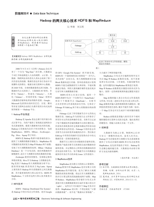
180 •电子技术与软件工程 Electronic Technology & Software Engineering数据库技术• Data Base Technique【关键词】Hadoop HDFS MapReduce 分布式数据存储 分布式数据处理2008年9月4日《自然》(Nature)杂志刊登了一个名为“Big Data ”的专辑,大数据这个词汇开始逐渐进入大众的视野,云计算、大数据、物联网技术的普及人类社会迎来了第三次信息化的浪潮,数据信息也在各行各业中呈现爆炸式的增长。
根据全球互联网中心数据,到2020年底,全球的数据量将达到35ZB ,大数据时代正式到来了,大数据的4V 特性:多样化(Variety )、快速化(Velocity )、大量化(V olume )、价值密度低(Value )使得对大数据的存储和处理显得格外重要,Google 、Microsoft 包括国内的阿里巴巴、百度、腾讯等多家互联网企业的巨头都在使用分布式处理软件框架——Hadoop 平台。
1 Hadoop平台简述Hadoop 是Apache 基金会旗下的开源分布式计算平台,为用户提供了系统底层透明的分布式基础架构。
随着大数据相关技术的发展,Hadoop 已发展成为众多子项目的集合,包括MapReduce 、HDFS 、HBase 、ZooKeeper 、Pig 、Hive 、Sqoop 等子项目。
HDFS 是Hadoop 集群中最基础的部分,提供了大规模的数据存储能力;MapReduce 将对数据的处理封装为Map 和Reduce 两个函数,实现了对大规模数据的处理;HBase (Hadoop Database )是一个分布式的、面向列数据的开源数据库,适合于大规模非结构化数据的存储;Zookeeper 提供协同服务,实现稳定服务和错误恢复;Hive 作为Hadoop 上的数据仓库;Pig 是基于Hadoop 的大规模数据分析平台,提供类似SQL 的查询语言Pig Latin ;Sqoop 主要用来在Hadoop 和关系数据库之间交换数据。
云计算的概念及关键技术

云计算的概念及关键技术1、云计算的概念1.1概念云计算是一种通过互联网访问、可定制的IT资源共享池,并按照使用量付费的模式,这些资源包括网络,服务器,存储、应用、服务等。
广泛意义上来说,云计算是指服务的交付和使用模式,即通过网络以按需,易扩展的方式获取所需的资源,这种服务可以是IT的基础设施(硬件、软件、平台),也可以是其他服务,云计算的核心理念就是按需服务,就像人使用水、电、天然气等资源一样。
1.2关键技术云计算的关键技术有:虚拟化、分布式文件系统、分布式数据库、资源管理技术、能耗管理技术。
虚拟化:虚拟化是实现云计算重要的技术设施,是在通过物理主机中同时运行多个虚拟机实现虚拟化,在这个虚拟化平台上,实现对多个虚拟机操作系统的监视和多个虚拟机对物理资源的共享;分布式文件系统:指在文件系统基础上发展而来的云存储分布式系统,可用于大规模的集群,主要特点:1、高可靠性:云存储系统支持多个节点间保存多个数据副本的功能,以提供数据的可靠性;‘’2、高访问性:根据数据的重要性和访问频率将数据分级多副本存储、热点数据并行读写,提高访问;3、在线迁移、复制:存储节点支持在线迁移,复制、扩容不影响上层应用;4、自动负载均衡:可以根据当前系统的负荷,将原有节点上的数据迁移到新增的节点上,特有的分片存储,以快为最小单位来存储,存储和查询时所有的存储节点并行计算;5、元数据和数据分离:采用元数据和数据分离的存储方式设计分布式文件系统。
分布式数据库:能实现动态负载均衡、故障节点自动接管、具有高可靠性,高可用性、高可扩展性;资源管理技术:云系统为开发商和用户提供了简单通用的接口,使得开发商将注意力更多低集中在软件本身,而无需考虑到底层架构,云系统一句用户的资源获取请求,动态分配计算资源;能耗管理技术:云计算基础设施中包括数以万计的计算机,如何有效低整合资源、降低运行成本,节省运行计算机所需的能源成为一个关注的问题二、hadoop生态在云计算这一块,hadoop算做的比较不错,hadoop平台的基本框图和生态系统如下所示:说明:1、MapReduce:是一个并行化计算框架,提供了map和reduce两阶段的并行处理模型和过程,mapreduce以键值对的数据输入方式来处理数据,并能自动完成数据的划分和调度管理;2、分布式文件系统(HDFS):基于物理上分布在各个数据存储节点的本地Linux系统的文件系统,为上次提供一个逻辑上成为整体的大规模数据存储系统;3、分布式数据库管理系统(HBASE):克服了难以管理结构化/半结构化海量数据的缺点,提供了一个大规模分布式的,建立在HDFS之上的分布式数据库管理系统,Hbase提供了基于行,列和时间戳的三维数据管理模型;4、公共服务模块(Common):为hadoop提供支撑服务和常用的工具类库以及api编程接口,服务包括:抽象文件系统fileSystem、远程过程调用(RPC),系统配置工具以及序列化机制;5、数据序列化(Avro):用于将数据结构和数据对象转变成数据存储和网络传输的格式;6、分布式协调服务(Zookeeper):主要用户提供分布式应用经常需要的系统可靠性维护,数据状态同步、统一命名服务,分布式应用配置等管理功能;7、分布式数据仓库处理工具(Hive):用于管理存在HDFS和hbase中的结构化/半结构化的数据。
大规模分布式存储系统概念及分类

大规模分布式存储系统概念及分类一、大规模分布式存储系统概念大规模分布式存储系统,是指将大量存储设备通过网络连接起来,形成一个统一的存储资源池,实现对海量数据的存储、管理和访问。
这种系统具有高可用性、高扩展性、高性能和低成本等特点,广泛应用于云计算、大数据、互联网等领域。
大规模分布式存储系统的主要特点如下:1. 数据规模大:系统可存储的数据量达到PB级别甚至更高。
2. 高并发访问:系统支持大量用户同时访问,满足高并发需求。
3. 高可用性:通过冗余存储、故障转移等技术,确保数据安全可靠。
4. 易扩展:系统可根据业务需求,动态添加或减少存储设备,实现无缝扩展。
5. 低成本:采用通用硬件,降低存储成本。
二、大规模分布式存储系统分类1. 块存储系统(1)分布式文件系统:如HDFS、Ceph等,适用于大数据存储和处理。
(2)分布式块存储:如Sheepdog、Lustre等,适用于高性能计算场景。
2. 文件存储系统文件存储系统以文件为单位进行存储,支持丰富的文件操作接口。
常见的文件存储系统有:(1)网络附加存储(NAS):如NFS、SMB等,适用于文件共享和备份。
(2)分布式文件存储:如FastDFS、MooseFS等,适用于大规模文件存储。
3. 对象存储系统对象存储系统以对象为单位进行存储,具有高可用性和可扩展性。
常见的对象存储系统有:(1)Amazon S3:适用于云存储场景。
(2)OpenStack Swift:适用于私有云和混合云场景。
4. 键值存储系统键值存储系统以键值对为单位进行存储,具有简单的数据模型和高速访问性能。
常见的键值存储系统有:(1)Redis:适用于高速缓存和消息队列场景。
(2)Memcached:适用于分布式缓存场景。
5. 列存储系统列存储系统以列为单位进行存储,适用于大数据分析和查询。
常见的列存储系统有:(1)HBase:基于Hadoop的分布式列存储数据库。
(2)Cassandra:适用于大规模分布式系统的高可用性存储。
- 1、下载文档前请自行甄别文档内容的完整性,平台不提供额外的编辑、内容补充、找答案等附加服务。
- 2、"仅部分预览"的文档,不可在线预览部分如存在完整性等问题,可反馈申请退款(可完整预览的文档不适用该条件!)。
- 3、如文档侵犯您的权益,请联系客服反馈,我们会尽快为您处理(人工客服工作时间:9:00-18:30)。
PLSA Search Engine2008 Parallel Programming Department of Computer Science and Information Engineering,National Taiwan UniversityProfessor: Pangfeng LiuSponsored by GoogleB92902036Shoou-Jong (John) Yu余守中B94902007Shih-Ping (Kerry) Chang張詩平B94902062Kai-Yang Chiang 江愷陽B94902063Yu-Ta (Michael) Lu呂鈺達B94902065Shoou-I Yu 余守壹Contents Introduction (3)Introduction to PLSA (3)Motivation (3)Implementation (3)Pre-Processing (5)Naïve PLSA (6)Overview (6)Implementation (6)Design process (8)Advanced PLSA (8)Overview (8)Implementation (9)Design Process (12)Query Fold-In and Search Engine (13)Performance Analysis and Comparison (14)Performance Analysis for Advanced PLSA (14)Comparison Between Naïve and Advanced PLSA (15)Comparison with OpenMP and MPI (16)Difficulties (17)Conclusion (21)Future Works (21)PLSA Implementation (21)In Query (22)What We Have Learned and Thoughts on Hadoop/Map-Reduce (22)By Michael Lu (22)By John Yu (23)By Shih-Ping Chang (24)By Kai-Yang Chiang (24)By Shoou-I Yu (25)Division of Labor (26)Reference (26)IntroductionIntroduction to PLSAProbabilistic latent semantic analysis (PLSA) is a statistical technique for the analysis of co-occurrence data. In contrast to standard latent semantic analysis, which stems from linear algebra and shrinks the size of occurrence tables (number of words occurring in some documents), PLSA is based on probability and statistics to derive a latent semantic model.Instead of the traditional key-word based data classification, PLSA tries to classify data to its “latent semantic”. It’s about learning “what was intended” rather than just “what actually has been said or written”. After performing the PLSA classification, words which often come together in a same document will be seen as highly connected to each other, and the documents which contain these words therefore will be classified into the same “topic”. The whole PLSA process can be divided into two parts, which are corpus classification and the query fold-in. Both parts use the expectation maximization (EM) theory. After running tens of iterations, we can get the final result.PLSA can be used in many areas, such as information retrieval or machine learning, to improve the original results.MotivationThe PLSA search engine was the final project that two of our teammates planed to do for the Digital Speech Processing class in 2007. However, when they started to implement the theory into code, they found that it takes too long to obtain the PLSA model because it is constructed by a huge amount of data. In order to finish the project in limited time, they were forced to reduce the size of the corpus data. Because of that, the outcome of the search engine was not accurate enough and the topic size was also limited. So we came up with an idea of using parallel programming to speed it up and hopefully by using a larger corpus data, we can get a better result.ImplementationThe following diagram shows the flow of our project.d: document, w: word, z: topicWe use the PTT Food board as the data source of our project. PTT is the biggest BBS site in Taiwan, and the Food board contains postings about people’s experience in variousrestaurants around Taiwan. After parsing the data so that some useless symbols are removed, we divided the sentences into several two-letter words and calculated the ()w d n , (number of word w appearing in document d ) of each document. Then we use the information and the given initial values to construct a PLSA model. This is the part where parallel programming takes place. After running a fixed number of iterations, we can get the final results. Finally, we made a query interface for demonstration.Below we shall explain in detail the flow and implementation of the whole project. Note that in the two sections that details the two algorithms we have implemented, each section will be organized as follows: “Overview” will provide a quick introduction of the algorithm; “Implementation” section will outline the detail of how PLSA is implemented under Map-Reduce; “Design Process” will discuss in detail the underlying philosophy of the implementation, along with other design tradeoffs and choices we have made that gave rise to the final implementation mentioned in the previous sectionPre-ProcessingWe wanted to get our training data from one of Taiwan's largest BBS site: PTT (telnet://). However, fetching data directly from BBS is inconvenient. Luckily every board in PTT has an approximate mapping on PTT's website(), we retrieve data from the website instead. Though it is not completely up to date with the BBS site, it is enough for our project.The process is as follows.1.Because we wanted to make a search engine to search the Food board, we used thetool “wget” on Linux to download all contents in the website's Food directory as well as its subdirectory to our own machine.2.Now, we have gotten all web pages about food from the web site. Our next step is toextract the contents we need from the original web pages. Since every page iscomposed of text and html tags, we have to remove all the tags inside the pages.Luckily, because all contents we want are between the tag pair <pre> and </pre> and every page has only 1 tag pair of this kind, we can remove all contents in the pagesbut the text between <pre> and </pre>.3.There are a large number of documents in our data folder. However, some of thesedocuments are useless for our purpose, such as indexing pages. We found that most of the pages we need have character counts between some intervals. Therefore, we only keep documents within that interval.ing all the documents, we build a dictionary consisting of 2-character words alongwith their appearing frequency in all the documents. We achieve this by scanningthrough all documents. Whenever a new character pair appears in a document, we add the word to our dictionary and set its frequency to be 1. When a character pair isalready in the dictionary, we add its frequency by 1. After scanning all documents, we remove words with lower frequency and only keep 20,000 words in the dictionary.5.The next step is to count how many times a word in the dictionary appears in 1document. Finally, we have the statistics of the word count of each document. Withthese statistics and the dictionary file, we are now able to start training the PLSAmodel.As for the initial probabilities of ()z d P,()z w P,()z P, ()z w P is initialized randomly, while ()z d P i and ()i z P are initialized to d1and z1respectively.Naïve PLSAOverviewIn this first version, we strive to be as intuitive and easy to code as possible. We observe that we have to compute four major components, namely the numerator and denominator of ()w d z P , and ()z d P ,()z w P ,()z P (they require similar computation), in one iteration of EM process. So we just simply divide the work so that each component is done in one Map-Reduce job. Thus this approach offers us a method to compute one iteration of EM process with four Map-Reduce jobs.Though this naïve algorithm is simple, it works correctly and this is our first version of PLSA. We will elaborate the implementation detail in next sub section.ImplementationConsider one iteration in EM process. First, we compute ()w d z P , by giving ()z d P ,()z w P ,()z P . These values come from the outcomes of the previous EM process. After we have ()w d z P , for each ()w d , pair, we can compute the new()z d P ,()z w P ,()z P in parallel.Let’s consider the E-step. ()w d z P , can be computed by the equation: ()()()()()()∑××××=t t t t z w P z d P z P z w P z d P z P w d z P ),( The algorithm uses 2 rounds of Map-Reduce to obtain all ()w d z P ,, one for the numerator and the other for the denominator. The first Map-Reduce is for the denominator. Each mapper will be responsible for an interval of documents, and for each document j d , it will compute all ()()()t i t j t z w P z d P z P ×× for each i w and t z . Next we set the z value as(1)the key, thus the reducer can sum up all ()()()t i t j t z w P z d P z P ×× for the same t z , output the summation to GFS and finally for each z we obtain a w d × entry table recording the denominator. The second pass computes the numerator and ()w d z P ,. We compute each()()()z w P z d P z P ×× for a given z in the mapper, and divide the computed denominator and output ()w d z P , for a given z in the reducer. Therefore we complete the E-step in the first two Map-Reduce passes.M-step, on the other hand, takes another two Map-Reduce passes. Consider three equations in M-step as the following:The third pass Map-Reduce computes the numerator of ()z w P and ()z d P . We divide z into several intervals for the mapper. For a given z , we compute ()()∑×j j j w d z P w dn ,, and ()()∑×ii i w d z P w d n ,,, throwing their value to the reducer with its type (numerator for()z w P or ()z d P ) and z as the keys respectively. Next we use a partitioner to partition intermediate value by its type so that we can deal with ()z w P and ()z d P in two different reducers. Finally, in the reducer, we output the numerator of ()z w P or ()z d P to their respective output files.The fourth pass is used to compute the numerator of ()z P , and to normalize ()z w P , ()z d P and ()z P (that is, divided by the denominator).The mapper computes the(2)(3)(4)denominator of the three equations by adding all the ()()∑×j j j w d z P w dn ,, computed in the previous Map-Reduce pass, the reducer does the normalization by loading in ()z d P , ()z w P , divide their value by the normalization factor, and output the normalized result back to the DFS.Each pass will be sequentially executed by the main method. Except for combining four pass Map-Reduce routine stated above, the main method is also responsible for running the EM process iteratively and setting the input/output file’s path for each Map-Reduce.Design processThis is the first step in our project. Since we have no prior experience in Map-Reduce design, our design process is simple: observe the equation, try to divide the problem to sub-problem, and make it possible to fit the Map-Reduce model.The main objective of the naïve algorithm is not its performance, but correctness.Therefore, we did not make much effort on optimizing time or space complexity. However, we achieved two important objectives with our naïve algorithm.The first one is that we found a solution to our problem, proving that PLSA is solvable with the Map-Reduce model. It is important and realistic to find a basic approach at first, and try to improve it afterwards. Second, we got to become familiar with Hadoop and theMap-Reduce model by working on the naïve version. It gave us an opportunity to design our next Map-Reduce algorithm with more understanding of its working details. We were eventually able to call on the experience gained with naïve PLSA to develop the advanced PLSA.Advanced PLSAOverviewWhile the naïve version PLSA produces the correct results, it is obvious from the analysis that there is ample room for improvement. Therefore after completing the naïve version, we embarked on overhauling the implementation of PLSA. In this new version, the most marked improvement is that now one iteration of PLSA is now completed in one iteration, and along with other improvements to reduce computation and I/O, the advancedPLSA showed an improvement of 74 times over the previous version.ImplementationThe input of mappers consists of two parts. First part is “mapper.txt”, which is commonly read and divided amongst all the mappers. “Mapper.txt” looks like the following:Where “00002” denotes the id of the mapper which receives this line, “d 09219 13937”means that this mapper is responsible for calculating ()z d P for documents 9219 to 13937. Similarly, “00020 w 00470 00722” means mapper id no. 20 is responsible for computing the ()z w P for words 470 to 722. Other necessary information is read through the file system. These files include ()w d n , for the given mapper, and ()z d P , ()z w P , ()z P from the previous iteration.Mapper computation is divided into two parts, and here we will use a mapper that is responsible for computing ()z d P for a given range as an example. Fig. 2 is a visualization of the most important component in the mapper, a 2-D array of topic ×words, and each cell in the array represents ()i j w d z P , in equation 1. In the first part of computation, each cell is updated by computing the new ()i j w d z P , from corresponding values of the previous iteration. As each cell is computed in row-wise fashion, their values are also summed together to obtain the normalization factor for this row. Once every cell of a row is computed and the normalization factor obtained, the whole row is normalized, thuscompleting the calculation for a row. This process is repeated for all the rows of the array toIt is also worth noting that the x-axis of the 2-D array is words in the given document instead of total words. Since average words in a document (551 words) is a lot less than the number of words in the dictionary (20,000 in this project), this advance in representation will save enormous amount of memory and computation, which will be analyzed in later sections.In part two of mapper computation, the matrix above is summed together column-wise to obtain the circled equation in Fig 3, and this value is then passed to the reducer. ()z w P is similarly obtained with the algorithm above.Fig 2. mapper computation part oneThe communication between mapper and reducer is done with the following format:Where the not yet normalized ()z d P and ()z w P is passed from the mapper to the reducer.The responsibility of the reducer is to normalize the incoming ()z d P and ()z w P. If we use the reducer responsible for ()z w P as an example, summing the i th column of the 2-D array shown in Fig. 5 would yield the normalization factor for that column of ()i z d P, in addition to the unnormalized value of ()i z P. This process repeats until all theunnormalized ()i z P and normalized ()i z d P is calculated and outputted to the file system for use by the next iteration. Finally, all the ()i z P is normalized and outputted to the file system as well. It is worth noting that there can be at a maximum of only two reducers, oneresponsible for ()z d P and one responsible for ()z w P. More reducers are not possibleFig 5. reducer computationDesign ProcessWhile elated with the completion of the naïve version, which proved that PLSA is indeed solvable with the Map-Reduce model, we were totally appalled by the poorperformance of the program, which was 83 times slower than a sequential version written with C. At the time, we believe that the problem was the inherit communication necessary between different rounds of Map-Reduce, which has to go through the file system, and the overhead accompanied in starting mapper and reducer tasks.Now, let’s partition the PLSA equations into smaller parts for the ease of explanation()()()z w P z d P z P i j ×× ( numerator of (1) )()()()∑××t t i t j t z w P z d P z P ( denominator of (1) )()()∑×j j j w d z P w d n ,, ( numerator of (3) )()()∑∑×j i i j i j w d z P w d n ,, ( denominator of (2), (3), numerator of (4))()()∑×i i i w d z P w d n ,,( numerator of (2) )After scrutinizing the equations of the PLSA algorithm, we found a way to load data into a mapper such that we can compute equation 5, 6, 9 or equation 5, 6, 7 with a single mapper, and gracefully hand over ()z d P or ()z w P respectively to the reducer. However, if we choose to compute equation 5, 6, 9 and gracefully pass on ()z d P , it is necessary to output a total of ()z w d O ×× pieces of data to piece together ()z w P , and vice versa if we choose to calculate equation 5, 6, 7. To make matters worse, the process of piecing together ()z w P can only be done by a single reducer (otherwise more communication, thus more rounds of Map-Reduce is necessary).Here we are faced with a dilemma, and there are two choices: one is to gracefully calculate either ()z w P or ()z d P and piece together the other one; the other is to make redundant calculations, so that both ()z w P and ()z d P can be passed gracefully to the(5) (6) (7) (8) (9)reducer, which would require only a total of ()()z w d O ×+ pieces of data. After lengthy consideration, we decided that if duplicating computation means we can avoid the inherently sequential work of piecing together ()z w P or ()z d P , we should avoid the inherentlysequential codes. In addition, this method is more intuitive, and with a relatively small test case of (d; w; z) = (2,000; 2,000; 100), we thought that having a reducer collect O(d*w*z) pieces of values seem like a huge bottleneck in terms of the whole project.In hindsight, after running test cases in the range of (d; w; z) = (80,000; 20,000; 700), we realize that collecting ()z w d O avg ×× pieces of values might not seem like a huge bottleneck after all, as mappers are now running in the range of 40 minutes per mapper. Doing away with the redundant computation would mean time and computation power to try to speed up the piecing together of ()z w P or ()z d P , which might yield better performance.Query Fold-In and Search EngineWith the result of the trained PLSA model, we can handle user queries in a search engine. We use PHP to build the search engine web page, and the following method is used to find the documents corresponding to the user's query.1. We treat one query as one document. We decompose the query into many pairs of2-character words, just as how we process documents.2. We now have the word count of the query, denoted ()w q n ,. We run EM algorithm for this query just like that we run EM for each document. The subtle difference is that ()z w P and ()z P remain static during the process. ()z q P is the only thing that will change in M-step and will also result in the change in E-step.3. We get what we need after step 2! We have ()z q P now and it means that we have gotten a vector indicating the proportion of each topic in this query. We also have()z d P for all the documents in our training corpus. We take the inner product of()z q P and ()z d P for each document as the relating score between the query and a document. Clearly, the document which produces the maximum score is the mostrelated document with the query.4. We sort the documents according to their score and only list the documents whosescore is higher than some given threshold. Moreover, we choose topic 1z which has the maximum ()1z q P and list the words with the highest ()1z w P s as similar wordsand display the result to user.Performance Analysis and ComparisonPerformance Analysis for Advanced PLSA Advanced PLSATiming for 10000 documents, 20000 words, 1000 topics - One IterationProcessorsAverage Time(s) 12387.0139404 2 1560.436385 41057.677541 8842.8095478 16731.2347188 32650.9973154Above are the timing results for the same test data using different amount of processors. The test data has 10000 documents, 20000 words and 1000 topics. It is quite clear that the non-parallelizable part of the code takes up quite a lot of time, because the improvement amount decreases as we increase the number of processors used. We can make a slight estimate of the length of the non-parallelizable part of the code, which we assume is mostly I/O overhead. Let K denote the communication time, and L denote the parallelizable part of the code. Let p be the amount of processors used. An estimation formula is p L K +. We derived that 621=K and 1766=L will give us the lowest absolute value difference compared to the experimental results. The non-parallelizable part of the code takes up about one-fourth of the whole sequential program! This is only a brief and not at all rigorous estimate, but we can get the idea that the I/O overhead of our program is still quite high.Advanced VersionTiming for Different Test Data - One IterationDocuments Words TopicsComputational Complexity Time(s) 2000 20000100 4E+09 58.624944 10000 200001000 2E+11 650.99732 82974 20000250 4.149E+11 935.93066 82974 200007001.162E+122559.9278Above are the timing results that we have run for each test data. For the PLSA model to be accurate, we ran all our test data for 50 iterations.We would have liked to use more topics for the test data with 82974 documents, but due to memory constraints, we were not able to do so. Our advanced method requires that the whole ()z d P and ()z w P array be in memory, and Hadoop has an constraint that all mappers can only use 1 GB of memory. Therefore we cannot use as many topics as we liked.Comparison Between Naïve and Advanced PLSATo see the improvement of advanced PLSA over naïve PLSA, we timed both algorithms for input size d = 2000, w = 20000 and z = 100. The results are as follows:VersionMachine Information Time (min) Naïve C with OpenMPGrid02 8 cores 14 Naïve PLSAGoogle cluster with 36 cores 74 Advanced PLSAGoogle cluster with 32 cores 1The followings are some possible factors contributing to this tremendous performance improvement. First is improvement of algorithm. Our advanced PLSA reduced the number of Map-Reduce pass to 1 instead of 4; that is, the advanced version eliminates many costs associated with running multiple Map-Reduce jobs. For instance, we now only need tosynchronize once per iteration instead of four times, which means the amount of time wasted waiting for mappers/reducers completing their works. Additionally, the advanced versionavoids lots of local disk I/O and GFS access which were originally necessary to communicate between each Map-Reduce job. Advanced version keeps all the necessary information in memory, and is quickly and readily available for the next stage of computation.Another important improvement is that the 2-D topic ×words array now only includes words that appear in a given document instead of all words that appear in the dictionary. This improvement prevents wasting computation power for entries whose ()0,=w d n .Empirically, there are only 551 words on average in one document. While the naïve version still does the computation for all 20000 words, advanced version takes advantage of this “sparse” property of ()w d n , and only computes those valid “w” entry. This means we have reduced the amount of computation by approximately 20,000/551 ~= 36 times.A smaller improvement is changing the representation of ()w d n ,. Since ()w d n , is a sparse matrix, we changed the representation from a 2-D array to a pair-wise representation of (word label, ()w d n , ). The reduction comes from the same fact mentioned above: adocument contains relatively little words compared to the dictionary, and this change greatly reduces the amount of file I/O needed by the mapper to obtain the required ()w d n , information.Comparison with OpenMP and MPIWhat if our project is done with OpenMP and/or MPI instead of Map-Reduce?OpenMP is indeed very suitable for computing PLSA, as all the information is stored on a common shared memory, minimizing communication costs between processors. Moreover, OpenMP is easy to parallelize, as all we have to do is write the sequential code and add the “pragma omp parallel for” clause in front of the “for” directive. In fact, we did write asequential version using a naïve algorithm and parallelize it using OpenMP, and it performs a lot better than our naïve PLSA. However, despite its low coding complexity, the scalability of OpenMP is limited by the number of cores that is connected to a single shared memory. Hence, scalability is a critical drawback of OpenMP.How about MPI? MPI is generally expected to have better performance thanMap-Reduce because it is coded in C. Also, any processor can communicate with any other processor, with no limit on time and format, while in Map-Reduce processor can onlycommunicate with others between the mapper and reducer, or via DFS. However, in MPI, any loss of passing message can result in deadlock or the failure of the whole computation, let alone sudden malfunction of machines. Map-Reduce, on the other hand, has a robust fault tolerance feature. The task can still be completed even if some machines in the cluster breaks down. Therefore, though MPI is faster and more flexible, it has high coding complexity and it is much more unreliable than Map-Reduce.DifficultiesThis section will primarily be focused on the difficulties we met when we tried to run our program on the Hadoop server. We met lots of problems when we implemented the naïve version of PLSA.Blank output file written by the mapper to the filesystemAt first, we were not really familiar with the Map-Reduce concept; therefore we wrote our program using the MPI concept. Since speed was not our main concern, we used the file system as the means of communication. Therefore, our mappers will read files from the file system and, while not using any reducers, write files directly to the file system.However, for some unknown reason, some files written to the file system are blank. We spent quite some time debugging but could not find the reason. After discussing this phenomenon with Victor (Google Engineer), he said that it is odd for a mapper to beoutputting files in the first place. Therefore we changed our code so that it fits more into the Map-Reduce concept: pass on the output to the reducer, and then let the reducer do the outputting for us.Even with the same keys, the order of the values received at the reducer may be different from the sending order of the mapper.We met another problem when we tried to send the data we computed from the mapper to the reducer. This problem occurred in the calculation of the ()w d z P , step. Each mapper will be given a topic number n , and that mapper will be responsible for calculating and outputting ()w d z P n ,. In order to avoid the blank output file problem, we had to somehow send the data produced at the mapper to the reducer. Let D and W denote the number of documents and words in our test data respectively. The array calculated will be of size D ×W , which is quite big. Therefore, instead of sending the whole array once to the reducer, we decided to send data of length W D times to the reducer, thus cutting the memory requirement at the mapper from D ×W to W . However, even though each mapper uses the topic number it is processing as its key, which will be unique, to send data to the reducer, the order of data received at the reducer is different from the order sent by the mapper. If the order is different, we would have to buffer all the ()w d z P , data in memory at the reducerbefore writing it to disk. When we discovered this problem, we avoided the sending process by doing all our calculation in the reducer. All the mapper does then is send the topic it is responsible to the right reducer with a partitioner. With this method, we successfully avoided this problem and decreased the amount of traffic between the mapper and reducer greatly.Task task_2008…0002_0 failed to report status for 601 seconds. Killing!With the above two problems out of the way, our naïve version runs correctly on very small test data, but when we tried to run data with about 800 documents and 10000 words, all our tasks were killed by the above message. Our TA showed us what the script in/hadoop/hadoop-0.16.0/conf/hadoop-default.xml wrote:<property><name>mapred.task.timeout</name><value>600000</value><description>The number of milliseconds before a task will be terminated if it neither reads an input, writes an output, nor updates its status string.</description></property>Armed with this new knowledge, we updated the status string usingreporter.setStatus(any status string) ever so often in our program and avoided the problem. And to our pleasant surprise, since the status string can be any string we like, it was something that we had been looking for ever since we started our project: a channel that the program can show us its status in real-time, like the printf in C. Our status showed to which document/word a mapper has processed, which was useful because at least we now know the program is running, ever so slowly in the case of the naïve version. Through this new tool, we can do some very simple profiling for our mapper and reducer. One important discovery, though quite obvious at hindsight, was that string concatenation in Java is slow, since it allocates a new string for every concatenation operation. We used string concatenation when we need to send an array of double from the mapper to the reducer, or when outputting data at the reducer. We did it by turning all double s into string representation separated by a space. In order to avoid this problem, we wrote a new function for string which manually manages the memory and the re-implemented string concatenation. We did try to write a new output value class, but we were not really successful and thus did not spend a lot of time on it.Uploading the program takes a long time!This is a very stupid problem, but it caused us a lot of frustration. Why does uploading a program take such a long time (3 minutes)? We discovered the reason when we tried to。