第二章 汽车纵向动力学(20070925)
第2 章 汽车纵向动力学

其中包括实验数据与理论数据。根据该报告,有以下的发动机转速-扭矩实验数据:
发动机转速 ne(r/min) 转矩 Ttq(N m)
1250
45.4
1500
49.3
2000
54.4
2500
56.6
3000
61.3
3500
63.7
4000
63.2
4500
60.8
5000
58.1
5500
55.7
2.变速器及主减速器
0.561 0.537 0.512
汽车行驶速度 ua(km/h)
15.691 18.83 25.106 31.383 37.659 43.936 50.212 56.489 62.765 69.042 70.297 由此作图如下
2挡 传动比 ig2=1.842
道路坡度 i
0.147 0.161 0.179 0.186 0.202 0.209 0.205 0.193 0.179 0.167 0.156
=
a
q + hg
,计算出相应的 q、
q
LL
Cφ2 值,如下。
1挡 传动比 ig1=3.090
汽车行驶速度 ua(km/h) 加速度 a(m s-2) 加速时等效坡度 q 加速时附着率 Cφ2
9.354 11.225 14.966 18.708 22.449 26.191 29.932 33.674 37.415 41.157 41.905
103.394
1005.324
105.274
958.397
由此做出汽车的驱动力图,如下
40.144 53.525 66.906 80.287 93.668 107.049 120.431 133.812 147.193 149.869
纵向动力学PPT课件可编辑全文

汽车燃油经济性的试验方法
式中:Ff 、Fw-----滚动阻力、空气阻力; m、r -----汽车质量、车轮半径;
δ----旋转质量换算系数;
ua -----车速;
Tr -----滑行时,各车轮摩擦阻力矩之和, 常忽略不计。
(3). 在测功机上设定好。 (4). 进行试验。
第5页/共58页
汽车燃油经济性的试验方法
第1页/共58页
汽车燃油经济性评价指标
指汽车在一定载荷 (我国规定轿车半载、 货车满载)下,以最高档在水平良好路面上等 速行驶100km的燃油消耗量。
以一些典型的循环行驶试验工况来模拟实 际汽车的运行状况,并以百公里燃油消耗量 (或MPG)来评定相应工况的燃油经济性。
第2页/共58页
汽车燃油经济性的试验方法
所以, 档位数,会改善汽车的动力性 和燃油经济性。
第41页/共58页
传动系档位数及各档传动比的选择 一般认为档与档之间的传动比不宜大于
汽车侧向动力学
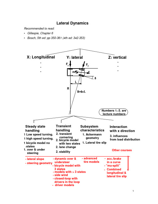
Lateral DynamicsRecommended to read:• Gillespie, Chapter 6• Bosch, 5th ed: pp 350-361 (4th ed: 342-353)Z: verticalInteractionwith x directionOther coursesX: Longitudinal Y: lateralSubsystem characteristicsSteady state handlingTransient handling1. over & under steering2. stability2. lane change1. Lateral tire slip 1 bicycle model no stateslateral tire slip2. bicycle modelwith two states 1. Ackermanngeometry- side wind2. transient cornering 1 Low speed turning. 1 high speed turning. - driver models- closed-loop with drivers in the loop3. influences from load distribution.General questionsSketch your view of the open- and closed-loop system, i.e. without and with the driver. Use a control system block diagram or similarOpen-loop vs closed loop studies of lateral dynamics. Closed-loop studies involve the driver response to feedback in the system. See text in Gillespie, p195, Bosch 5th ed p 354 (4th ed p 346).This course will only treat open-loop vehicle dynamics. How can we upgrade to closed-loop? For example: driver models, simulators or experimentsQuestions on low speed turningDraw a top view of a 4 wheeled vehicle during a turning manoeuvre. How should the wheel steering angles be related to each other for perfect rolling at low speeds?Ackermann steering geometry Array Deviations from Ackerman geometry affect tire wear and steering system forcessignificantly but less influence on directional response.Consider a rigid truck with 1 steered front axle and 2 non-steered rear axles. How do we predict the turning centre?Assume: low speed, small steering angles, low traction.We still cannot assume that each wheel is moving as it is directed. A lateral slip iscreated at all axles. The turning centre is then not only dependent of geometry, but also forces. The difference in the 3 axle vehicle compared to the two axle vehicle is that we now have 3 unknown forces but only 2 relevant equilibrium equations. In other words, the system is not statically determinateApprox. for small angles:Equilibrium: Fyf+Fyr1=Fyr2 and Fyf*lf+Fyr2*lr=0 Compatibility: (αr1+αr2)*lf/lr+αr1=δf -αf Constitutive relations: F yf =C αf *αfF yr1=C αr1*αr1F yr2=C αr2*αr2C α = cornering stiffness [N/rad]Together,3 eqs and 3 unknowns (the three slip angles) can be obtained for the figure below. Note that we assume a lateral force vector at each axle by choosing a slip angle:C αf *αf - C αr1*αr1 + C αr2*αr2 = 0 (Sum of forces in Y direction) C αf *αf *lf - C αr2*αr2*lr= 0 (sum of moments about r1) (αr1+αr2)*lf/lr + αr1 = δf - αf (compatibility)Steady state cornering at high speedIn a steady state curve at high speed, centripetal forces are needed to keep the vehicle on the curved track. Where do we find them? How large must these be? How are they developed in practice?Same C α at all axlesTest, e.g. prescribe steering angle. Calculate slip angles:VfThe centripetal force = F c=m*R*Ω2= m*Vx2/R. It has to be balanced by the wheel/road lateral contact forces:Equilibrium: Fyf+Fyr = F c = m*Vx2/R and Fyf*b-Fyr*c=0(Why not Fyf*b-Fyr*c=I*dΩ/dt ??? )Constitutive equations: F yf=Cαf*αf and F yr=Cαr*αrCompatibility: tan(δ−αf)=(b*Ω+Vy)/Vx and tan(αr)=(c*Ω-Vy)/Vxeliminating Vy for small angles and using Vx=R*Ω: δ−αf+αr=L/RTogether, eliminate slip angles:Fyf=(lr/L)*m*Vx2/R and Fyr=(lf/L)*m*Vx2/Rδ−F yf/Cαf+F yr/Cαr=L/REliminate lateral forces:d = L/R +[(lr/L)/Caf - (lf/L)/Car] * m*Vx2/Rwhich also can be expressed as: δ = L/R + [Wf/Cαf - Wr/Cαr] *Vx2/(g*R)(Wf and Wr are vertical weight load at each axle, respectively.)Wf/Cαf - Wr/Cαr is called understeer gradient or coefficient, denoted K or K us and simplifies to: d = L/R + K *Vx2/(g*R)A more general definition of understeer gradient:Note that this relation between δ , R and Vx is only first order theory. (Why?) Study a 2 axle vehicle in a low speed turn. How do we find the steering angle needed to negotiate a turn at a given constant radius? How do the following quantities vary with steering angle and longitudinal speed:•yaw velocity or yaw rate, i.e. time derivative of heading angle•lateral accelerationFor a low speed turn:Needed steering angle: δ = L / R (not dependent of speed)Yaw rate: Ω = Vx / R = Vx * δ / L (prop. to speed and steering angle)Lateral acceleration: ay = Vx2 / R = Vx2 * δ / L (prop. to speed and steering angle) Since steering angle is the control input, it is natural to define “gains”, i.e. division by δ:Yaw rate gain = Ω/δ =Vx/LLateral acceleration gain: ay/δ = Vx2/LFor a high speed turn:δ = L/R + K *Vx2/(g*R)Yaw rate gain = Ω/δ =(Vx/R) / δ=Vx/(L + K *Vx2/g)Lateral acceleration gain: ay/δ = (Vx2/R) / δ= Vx2/(L + K *Vx2/g)These can be plotted vs Vx:What happens at Critical speed? Vehicle turns in an unstable way, even with steering angle=0.What happens at Characteristic speed? Nothing special, except that twice the steeringangle is needed, compared to low speed or neutral steering..How is the velocity of the centre of gravity directed for low and high speeds?See the differences and similarities between side slip angle for a vehicle and for a single wheel. Bosch calls side slip angle “floating angle”.Some (e.g., motor sport journalists) use the word under/oversteer for positive/negative vehicle side slip angle.Transient corneringNOTE: Transient cornering is not included in Gillespie. This part in the course is defined by the answer in this part of lecture notes. For more details than given on lectures, please see e.g. Wong.To find the equations for a vehicle in transient cornering, we have to start from 3 scalar equations of motion or dynamic equilibrium. Sketch these equations.vm*dV I*d NOTE: It will m*dv/dt (2D vector equation)We like to express them without introducing the heading angle, since we thenwould need an extra integration when solving (to keep track of heading angle). In conclusion, we would like to use “vehicle fixed coordinates”.But the torque equation is straight forward:m*dV y /dt=Fyr+Fxf*sin(δ)+Fyf*cos(δ)x /dt=Fxr+Fxf*cos(δ)-Fyf*sin(δ)Ω/dt= -Fyr*c+Fxf*sin(δ)*b+Fyf*cos(δ)*bv is a vector. Let F also be vectors.NOT be correct if we only consider each component of v (Vx and Vy)separately, like this:=ΣF equation )I*d Ω/dt = ΣMz (1D scalar would like to express all equations as scalarequations . We would alsoMotion of a body on a plane surface:If we consider a rigid body (like a car) travelling on the road, we can analyse the motion of a reference frame attached to the vehicle.The body fixed to the x,y axes start with an orientation θ relative to the Global (earth fixed)system. The body has velocities V x and V y in the x,y system. Relative to the x,y system the point P has velocities:Ω−=y Vx vxΩ+=x Vy vyat time t t δ+, the velocities for P are:)()(Ω+Ω−+=′δδy Vx Vx x v )()(Ω+Ω++=′δδx Vy Vy y vSince the velocities have rotated by the angle δθ, the transformation of the velocities for P at time t t δ+to the original orientation:Time t+YTime tδ t)cos()sin()sin()cos(δθδθδθδθy v x v y v y v x v x v t t ′+′=′′−′=′where subscript “t” refers to coordinate system at time tThe difference of velocities for P in the time interval will then bevyy v vy vx x v vx −′=−′=δδSubstituting the values above:[][]()[][]()Ω+−Ω+Ω+++Ω+Ω−+=Ω−−Ω+Ω++−Ω+Ω−+=x Vy x Vy Vy y Vx Vx vy y Vx x Vy Vy y Vx Vx vx )cos()()()sin()()()sin()()()cos()()(δθδδδθδδδδθδδδθδδδIf consider that t δis very small, then )cos(δθ=1 and )sin(δθ=δθ and divide by t δtVy t x t y t y t Vx t Vx t vy t x t x t Vy t Vy t y t Vx t vx δδδδδδθδδδδδθδδδδδδδθδδδθδδθδδδθδδδδδδ+Ω+Ω−ΩΩ−+Ω=Ω−Ω−−−Ω−=()()()(if we let t=0 and let the global and local coordinate systems align at t=0 we can write dtd t ()()=δδ. We can also defineΩ=tδδθand ignore the second order terms ()()δδ⋅:22Ω−Ω+Ω+=Ω−Ω−Ω−=y dtd x Vx dt dVy ay x dtd y Vy dt dVx axAnd at the center of x,y system x=0, y=0:Ω+=Ω−=Vx dtdVyay Vy dtdVxaxNow, it will be correct if:m*a x = m*(dVx/dt - Vy*Ω) = Fxr + Fxf*cos(δ) - Fyf*sin(δ) m*a y = m*(dVy/dt + Vx*Ω)=Fyr + Fxf*sin(δ) + Fyf*cos(δ) I*d Ω/dt = - Fyr*c + Fxf*sin(δ)*b + Fyf*cos(δ)*bTry to understand the difference between (ax,ay) and (dVx/dt,dVy/dt).[The quantities (ax,ay) are accelerations, while (dVx/dt,dVy/dt) are “changes in velocities”. The driver will have the instantaneous feel of mass forces according to (ax,ay) but he will get the visual input over time according to (dVx/dt,dVy/dt).][Example: If going in a curve with constant longitudinal speed with driver in vehicle centre of gravity: The driver feel only “ax=0 and ay=centrifugal force=radius*Ω*Ω“ in his contact with the seat. However, he sees no changes in the velocity with which outside objects move, i.e. “dVx/dt=0 and dVy/dt=ay-Vx*Ω=radius*Ω*Ω-radius*Ω*Ω=0“.]Constitutive equations: F yf=Cαf*αf and F yr=Cαr*αrCompatibility: tan(δ−αf)=(b*Ω+V y)/V x and tan(αr)=(c*Ω-V y)/V xEliminate lateral forces yields:m*(dV x/dt - V y*Ω) = F xr + F xf*cos(δ) - Cαf*αf*sin(δ)m*(dV y/dt + V x*Ω) = Cαr*αr + F xf x*sin(δ) + Cαf*αf*cos(δ)I*dΩ/dt = -Cαr*αr*c + Fxf*sin(δ)*b + Cαf*αf*cos(δ)*bEliminate slip angles yields (a 3 state non linear dynamic model):m*(dV x/dt - V y*Ω) = Fxr + Fxf*cos(δ) - Cαf*[δ−atan((b*Ω+V y)/V x)]*sin(δ)m*(dV y/dt + V x*Ω) = Cαr*atan((c*Ω-V y)/V x) + Fxf*sin(δ) + Cαf*[δ−atan((b*Ω+V y)/V x)]*cos(δ) I*dΩ/dt = -Cαr*atan((c*Ω-V y)/V x)*c + Fxf*sin(δ)*b + Cαf*[δ−atan((b*Ω+V y)/V x)]*cos(δ)*b For small angles and dV x/dt=0 (V x=constant) and small longitudinal forces at steered axle (here Fxf =0), we get the 2 state linear dynamic model:m*dV y/dt +[(Cαf+Cαr)/V x]*V y + [m*V x+(Cαf*b-Cαr*c)/V x]*Ω=Cαf*δI*dΩ/dt +[(Cαf*b-Cαr*c)/V x]*V y + [(Cαf*b2+Cαr*c2)/V x]*Ω =Cαf*b*δThis can be expressed as:What can we use this for?- transient response (analytic solutions)- eigenvalue analysis (stability conditions)If we are using numerical simulation, there is no reason to assume small angles. Response on ramp in steering angle:• True transients (step or ramp in steering angle, one sinusoidal, etc.) (analysed in time domain) • Oscillating stationary conditions (analysed i frequency domain, transfer functions etc., cf. methods in the vertical art of the course).Examples of variants? Trailer (problem #2), articulated, 6x2/2-truck, all-axle-steering, ...ExampleShow that critical speed for a vehicle is sqrt(-L*g/K), using the differentialequation system valid for transient response. Assume some numerical vehicle parameters. Which is the mode for instability (eigenvector, expressed in lateral speed and yaw speed)?How to find global coordinates? dX/dt=Vx*cos ψ - Vy*sin dY/dt=Vy*cos ψ + Vx*sin X (global,Y (global,earth fixed) earth fixed)heading angle, Vx VyΩSolution sketch (using Matlab notation):» [m I g L l Cf/1000 Cr/1000] = 1000 1000 9.8 3 1.5 100000 80000(These are the assume vehicle parameters in SI units)» K=m*g/2*(1/Cf-1/Cr) = -0.0122 (understeer coefficient)» A=[m 0;0 I] =1000 00 1000 (mass matrix)» Vx=sqrt(-L*g/K)= 48.9898 (critical speed according to formula)» B=-[(Cf+Cr)/Vx m*Vx+(Cf*l-Cr*l)/Vx ;(Cf*l-Cr*l)/Vx (Cf*l*l+Cr*l*l)/Vx];» C=inv(A)*B; [V,D]=eig(C)0.9973 0.9864-0.0739 0.1644D = (diagonal elements are eigenvalues)0.0000 00 -11.9413Note that the first eigenvalue is zero, which means border between stability and instability. This is the proof!The eigenvector is first column of V, i.e. Vy=0.9973 and Ωz=-0.0739 (amplitudes):ExampleVehicles that have lost their balance might sometimes be stabilized through one-sided brake interventions on individual wheels (ESP systems). Which wheels and how much does one have to brake in the following situation?Vx=30 m/s, cornering radius=100 m.Before time=0: Cf=Cr=100000 /radAt time=0, the vehicle loses its road grip on the front axle, which can be modelled as a sudden reduction of cornering stiffness to 50000 N/rad.Assume realistic (and rather simplifying!) vehicle parameters.Solution (very brief and principal):Assume turning to the right, i.e. right side is inner side. Use the differential equation system for transient vehicle response, but add a term for braking m*dV y /dt + [(C αf +C αr )/V x ]*V y + [m*V x +(C αf *b-C αr *c)/V x ]*Ω=C αf *δ I*d Ω/dt + [(C αf *b-C αr *c)/V x ]*V y + [(C αf *b 2+C αr *c 2)/V x ]*Ω =C αf *b*δ ++ Mzwhere Mz=Fr*B/2, Fr=brake forces at the two right wheels, B=track width For t<0: Solve the eqs with dV y /dt = d Ω/dt = Mz=0 and Cf=Cr=100000 and Ω=Vx/radius=30/100 rad/s. This gives values of δ and Vy.For t=0: Insert the resulting values for δ and Vy into the same equation system but with Cf=50000 and do not constrain Mz to zero. Instead calculate Mz, which gives a certain brake force on the two right wheels, Fr.Check whether Fr is possible or not (compare with available friction, µ*normal force). If possible, put most of Fr on the rear wheel since front axle probably has the largest risk to drift outwards in the curve.Longitudinal & lateral load distribution during corneringWhen accelerating, the rear axle will have more vertical load. Explore what happens with the cornering characteristics for each axle. Look at Gillespie, fig 6.3. ...C Part of: Gillespie, fig 6.3o r n e r i n g s t i f f n e s sVertical loadSo, the cornering stiffness will increase at the rear axle and decrease at front axle, due to the longitudinal vertical load distribution during acceleration. This means lesstendency for the rear to drift outwards in a curve (and increased tendency for front axle) when accelerating.The opposite reasoning applies for braking (negative acceleration.)So, longitudinal distribution of vertical loads influence handling properties.NOTE: A larger influence is often found from the combined longitudinal and lateral slip which occurs due to the traction force needed to accelerate.In a curve, the outer wheels will have more vertical load. Explore what happens with the lateral force on an axle, for a given slip angle, if vertical load is distributed differently toSo, lateral distribution of vertical loads influence handling properties.How to calculate the vertical load on inner and outer side wheels, respectively, when the vehicle goes in a curve?First consider the loads on the vehicle body and axle:Force in Springs)(x x Ks Fi ∆+=, )(x x Ks Fo ∆−= where x is the static displacement of the springand Dx is the change in spring length due to body rollSum moments about chassis CGM sx x Ks s x x Ks =∆−−∆+2)(2)(2φs x =∆M K sKs ==φφ2where K φ is the roll stiffness for the axleMoment applied from body to axle=K φ φIf we take the sum of the moments about point A:ΣM A =00222=++−φφK hr RV m t Fzi t FzoThis simplifies to:02)(2=+=−φφK hr RV m t Fzi Fzo022)(2=+=−tK t hr R V m Fzi Fzo φφwe can define the term ∆Fz as∆Fz= (Fzo-Fzi)/2where ∆Fz is where the change of vertical load for each tire on the axleHow can we account for the whole vehicle? If we assume that the chassis is rigid, we can assume that it rotates around the roll centers for each axle. This is shown in the figure below:Roll moment about x axis M φ = {mV 2/R h 1 cos(φ) + mg h 1 sin(φ)} cos(ε)for small angles• M φ = mV 2/R h 1 + mg h 1 φ– Let W=mg• M φ = W h 1 (V 2/Rg+ φ)• If we know M φ = M φf+ M φr• M φ = (K φf +K φr )φthen:(K φf +K φr )φ= W h 1 (V 2/Rg+ φ)(K φf +K φr - W h 1 ) φ= W h 1 V 2/Rg)(121Wh K K Rg VWh r f −+=φφφThis is the roll angle based on the forward speed and curve radius.From previous expression for one axle2∆Fz= 2mV 2/R hr/t + 2K φ φ/twhere hr is the roll axis height. For front axle, Substitute the value the following into the previous equation.For front axle: mV 2/R=Wf/gV 2/RThis results in the relationship: )(11212Wh K K Rg V Wh t K t h Rg V W F r f f f f Zf −+⋅+⋅=∆φφφSimilarly for rear axle:)(11212Wh K K Rg V Wh t K t h Rg V W F r f r r r Zr −+⋅+⋅=∆φφφThese equations allow the exact load on each tire to be calculated. Then the cornering stiffness can be calculated if a functional relationship is known between the cornering stiffness C α and Fz.How is vertical load distributed between front/rear, if we know distribution inner/outer?It depends on roll stiffness at front and rear. Using an extreme example, without any roll stiffness at rear, all lateral distribution is taken by the front axle. .In a more general case:Mxf=kf*φ Mxr=kr*φ , where kf and kr are roll stiffness and φ=roll angle.Eliminating roll angle tells us that Mxf=kf/(kf+kr)*Mx and Mxr=kr/(kf+kr)*Mx, i.e. the roll moment is distributed proportional to the roll stiffness between front and rear axle. We can express each Fz in m*g, ay, geometry and kf/kr. This is treated in Gillespie, page 211-213.How would the diagrams in Gillespie, fig 6.5-6.6 change if we include lateral load distribution in the theory?It results in a new function =func(Vx), (eq 6-48 combined with 6-33 and 6-34). It could be used to plot new diagrams like Gillespie, fig 6.5-6.6:Equations to plot these curves are found in Gillespie, pp 214-217. Gillespie uses the non linear constitutive equation: Fy=Cα*α where Cα=a*Fz-b*Fz2 .What more effects can change the steady state cornering characteristics for a vehicle at high speeds?See Gillespie, pp 209-226: E.g. Roll steer and tractive (or braking!) forces. Braking in a curve is a crucial situation. Here one analyses both road grip, but also combined dive and roll (so called warp motion).Try to think of some empirical ways to measure the curves in diagrams in Gillespie, fig 6.5-6.6.See Gillespie, pp 27-230:Constant radius• Constant speed• Constant steer angle (not mentioned in Gillespie)How to calculate the vertical load on front and rear axles, respectively, when the vehicle accelerates?In general: ΣFz=mg and ΣFz,rear=mg/2+(h/L)*m*ax, where L=wheel base and h=centre of gravity height. ax=longitudinal acceleration. Still valid for braking because ax is then negative.Component CharacteristicsPlot a curve for constant side slip angle, e.g. 4 degrees, in the plane of longitudinal force and lateral force. Do the same for a constant slip, e.g. 4%. Use Gillespie, fig 10.22 as input.See Gillespie Fig 10.23Summary•low speed turning: slip only if non-Ackermann geometry•steady state cornering at high speeds: always slip, due to centrifugal acceleration of the mass, m*v2/R•transient handling at constant speed: always slip, due to all inertia forces, both translational mass and rotational moment of inertia•transient handling with traction/braking: not really treated, except that the system of differential equations was derived (before linearization, when Fx anddVx/dt was still included)•load distribution, left/right, front/rea r: We treated influences by steady state cornering at high speeds. Especially effects from roll moment distribution.Recommended exercise on your own: Gillespie, example problem 1, p 231. (If you try todetermine “static margin”, you would have to study Gillespie, pp 208-209 by yourself.)。
3 汽车纵向动力学解读

FaV a < μFPH b ⋅ sin β ≈ μFPH bβ
当 F aH b > μ F pV a ⋅ sin β ≈ μ F 其中:
pV
aβ
FaV
= kV β
即满足kV a < μFPH b 时,汽车才处 于稳定状态
图 3-3-2
2009-10-19 18
第三章
汽车纵向动力学 四、驱动,后轮滑转
2009-10-19
( μ H − μ G λ T ) − ( μ H − μ G )λ (1 − λ T )
23
第三章
汽车纵向动力学
在此前提下,车辆和车轮的数学
模型可表达为:
I ω & = − T b + RF mv &= − Fb Fb
= μ ( λ ) Fz
b
制动力矩Ie It Iw
Id
aX
发动机旋转零件转动惯量
变速器旋转零件换算到其输入 端的等效转动惯量
车轮及半轴的转动惯量 传动轴转动惯量 车辆加速度
itf η tf
2009-10-19
5
第三章
汽车纵向动力学
2. 汽车的行驶阻力 汽车在水平道路上行驶时,必须克服来自地面的滚动阻力和来 自空气的空气阻力,当汽车在坡道上上坡行驶时,还必须克服重力 沿坡道的分力,称其为坡度阻力。
而
Td = Ft r / i f
Ts = Ts f + Tsr = Kφ r φ + Kφ f φ = Kφ φ
Ft r Kφ f i f t Kφ r+Kφ f
综合以上几式可得: Wy =
注意: 1. 横向载荷转移的大小是驱动力及一些其它车辆参数的函数; 2. 如果驱动桥的差速器未锁止,传至两侧车轮的转矩将受限于 垂直载荷较小一侧车轮的附着极限。
汽车纵向动力学97页PPT

6、最大的骄傲于最大的自卑都表示心灵的最软弱无力。——斯宾诺莎 7、自知之明是最难得的知识。——西班牙 8、勇气通往天堂,怯懦通往地狱。——塞内加 9、有时候读书是一种巧妙地避开思考的方法。——赫尔普斯 10、阅读一切好书如同和过去最杰出的人谈话。——笛卡儿
汽车纵向动力学
11、获得的成功越大,就越令人高兴 。野心 是使人 勤奋的 原因, 节制使 人枯萎 。 12、不问收获,只问耕耘。如同种树 ,先有 根茎, 再有枝 叶,尔 后花实 ,好好 劳动, 不要想 太多, 那样只 会使人 胆孝懒 惰,因 为不实 践,甚 至不接 触社会 ,难道 你是野 人。(名 言网) 13、不怕,不悔(虽然只有四个字,但 常看常 新。 14、我在心里默默地为每一个人祝福 。我爱 自己, 我用清 洁与节 制来珍 惜我的 身体, 我用智 慧和知 识充实 我的头 脑。 15、这世上的一切都借希望而完成。 农夫不 会播下 一粒玉 米,如 果他不 曾希望 它长成 种籽; 单身汉 不他 不曾希 望因此 而有收 益。-- 马钉路 德。
汽车理论个章节总结
第一章汽车的动力性1汽车动力性:指汽车在良好路面上直线行驶时由汽车受到的纵向外力决定的、所能达到的平均行驶速度。
2汽车动力性主要由三方面指标来评定:1)汽车的最高车速µamax:是指在水平良好的路面(混凝土或沥青)上汽车能达到的最高行驶车速2)汽车的加速时间t:表示汽车的加速能力。
常用原地起步加速时间与超车加速时间来表明汽车的加速能力原地起步加速时间指汽车由Ⅰ挡或Ⅱ挡起步,并以最大的加速强度(包括选择恰当的换挡时机)逐步换至最高挡后到某一预定的距离或车速所需的时间。
超车加速时间指用最高档或次高挡由某一较低车速权利加速至某一高速所需的时间3)汽车的最大爬坡度ⅰmax:是指Ⅰ挡最大爬坡度。
汽车的上坡能力实用满载(或某一载质量)时汽车在良好路面上的最大爬坡度ⅰmax表示的。
3汽车的驱动力:地面对驱动轮的反作用力Ft(方向与Fo相反)即是驱动汽车的外力,此外力称为汽车的驱动力。
4汽车驱动力公式Ft=5汽车驱动力图6汽车的行驶阻力的分类1)滚动阻力Ff2)空气阻力Fw(汽车直线行驶时受到的空气作用力在行驶方向上的分力)空气阻力分为压力阻力与摩擦阻力两部分压力阻力又分为四部分:形状阻力、干扰阻力、内循环阻力、诱导阻力3)坡度阻力Fi(汽车重力沿坡道的分力表现为汽车的坡度阻力)道路阻力:由于坡度阻力和滚动阻力均属于与道路有关的阻力,而且均与汽车重力成正比,故可以把这两种阻力合在一起称作道路阻力4)加速阻力Fj(汽车加速行驶时,需要克服其质量加速运动时的惯性力) 7汽车行驶方程式 Ft=Ff+Fw+Fi+Fj (N)Ff=Wf f-滚动阻力系数 W-车轮负荷Fw=CDAua²/21.15 CD-空气阻力系数 A-迎风面积m² ua-汽车行驶速度km/h Fi=Gsinα G-汽车重力Fj=δm du/dt δ-汽车旋转质量换算系数 m-汽车质量kg du/dt 行驶加速度m/s ²第二章汽车的燃油经济性1汽车的燃油经济性:在保证动力性的条件下,汽车以尽量少的油消耗量经济行驶的能力2汽车燃油经济性的评价指标:汽车的燃油经济性常用一定运行工况下汽车行驶百公里的燃油消耗量或一定燃油量能使汽车行驶的里程来衡量。
3 汽车纵向动力学解析

u x
& p=φ
w z
γ=ψ &
x y
υ
y q=ϕ &
z
∑M I q′ − ( I − I ) pγ = ∑ M I γ ′ − (I − I ) pq = ∑ M
I x p′ − ( I y − I z )qγ =
y z x y
x y
∑ Fx )= z m s(w′ − u ⋅ q ) = ∑ F
y q =ϕ &
SAE坐标系
13
第三章
汽车纵向动力学
二、空间任一刚体的运动方程
ms (u′−υ⋅γ + w⋅q) = ms ms
∑F (v′−w⋅ p+u⋅γ ) = ∑F (w′−u⋅q+υ ⋅ p) = ∑F
z x
x y z
∑M I q ′ − ( I − I ) pγ = ∑ M I γ ′ − (I − I ) pq = ∑ M
2009-10-19 6
第三章
汽车纵向动力学
作用在每个驱动轮上的垂直载荷等于静态载荷加上动态载荷, 后者是由加速时的纵向载荷转移或驱动转矩造成的横向载荷转移引 起的。 (1) 驱动转矩引起的横向载荷转移 不管是前桥还是后桥,只要驱动桥是刚性桥就存在横向载荷转 移。绕车桥中心点的力矩平衡方程为:
∑T O = ( W
这部分在汽车理论和第二章 轮胎动力学中有相应介绍,在此不
再重复。
二、汽车加速性能
知道了驱动力和行驶阻力,就可以计算车辆的加速性能了。 1.取决于发动机功率的极限加速能力 2.取决于附着力的极限加速能力 假设发动机功率足够大,极限加速能力会受到轮胎与路面之间
摩擦系数的限制。这样的话,驱动力的极限值为:
汽车纵向动力学研究综述

Internal Combustion Engine&Parts・23・汽车纵向动力学研究综述Research Progress of Automobile Longitudinal Dynamics于旺YU Wang(沈阳理工大学汽车与交通学院车辆工程专业,沈阳110159)(Vehicle Engineering,School of Automobile and Transportation,Shenyang University of Technology,Shenyang110159,China)摘要:随着汽车工业的发展,汽车纵向动力学研究不断加深,汽车在道路上行驶,就会存在驱动、制动、滑移等纵向动力学方面的问题。
针对这一问题的研究,人们提出了汽车纵向动力学的概念。
汽车纵向动力学的研究主要包括:汽车制动动力学、汽车防抱死系统、汽车驱动防滑系统、汽车自适应巡航系统、汽车自动刹车系统。
本文将主要介绍汽车纵向动力学控制系统组成和原理、汽车制动动力学控制系统的研究进展、汽车防抱死系统的研究进展、汽车驱动防滑系统的研究进展、汽车自适应巡航控制系统的研究进展、汽车自动刹车辅助系统的研究进展。
Abstract:With the development of the automotive industry,the research on the longitudinal dynamics of automobiles has continued to deepen,and there are problems with longitudinal dynamics such as driving,braking,and slipping when the car is driving on the road.In view of this problem,people have proposed the concept of automobile longitudinal dynamics.The research of automobile longitudinal dynamics mainly includes:automobile braking dynamics,automobile anti-lock braking system,automobile driving anti-skid system, automobile adaptive cruise system,automobile automatic braking system.This article will mainly introduce the composition and principle of automotive longitudinal dynamics control system,the research progress of automotive brake dynamics control system,the research progress of automotive anti-lock system,the research progress of automotive drive anti-skid system,the research of automotive adaptive cruise control system Progress,research progress of auto brake assist systems.关键词:汽车;纵向动力学;防抱死;驱动防滑;制动动力学;自适应巡航;自动刹车;系统Key words:automobile;longitudinal dynamics;anti-lock braking;driving anti-skid;braking dynamics;adaptive cruise;automatic braking;system中图分类号:U469.72文献标识码:A文章编号:1674-957X(2020)24-0023-020引言目前城市的发展和道路的优化设计极大地考验了汽车在道路上的行驶性能,要想在现有的道路上道路上提高交通流量并控制交通事故的发生,这就要求汽车设计者能在提高汽车安全行驶的车速和减小汽车与前后车之间的距离(但能有足够的安全距离)的同时能够保证汽车的各方面的稳定性能。
- 1、下载文档前请自行甄别文档内容的完整性,平台不提供额外的编辑、内容补充、找答案等附加服务。
- 2、"仅部分预览"的文档,不可在线预览部分如存在完整性等问题,可反馈申请退款(可完整预览的文档不适用该条件!)。
- 3、如文档侵犯您的权益,请联系客服反馈,我们会尽快为您处理(人工客服工作时间:9:00-18:30)。
发动机的外特性是通过发动机台架实验 获得的。 在已知发动机最大功率和对应声速时,发 动机的外特性可根据以下式估算:
2 3 ⎡ ⎛ n ⎞ ⎛ n ⎞ ⎛ n ⎞ ⎤ Pe = Pe max ⎢ A⎜ ⎟ + B⎜ ⎟ − ⎜ ⎟ ⎥ ⎟ ⎜n ⎟ ⎜n ⎟ ⎥ n ⎢ ⎜ p ⎝ p⎠ ⎝ p⎠ ⎦ ⎣ ⎝ ⎠
汽车的动力性
3.最大爬坡度imax 汽车的上坡能力。以1档满载时汽车 在良好路面上的最大爬坡度表示。是 极限爬坡能力。 轿车:一般不强调 货车: imax =30%(约16.5°) 越野汽车:imax =60% 有时也以汽车在一定坡道上必须达到 的车速来表示爬坡能力。如:美国对 轿车爬坡要求,能以104
同济大学,汽车学院 左曙光教授教案
汽车的驱动力图
发动机外特性确定的是发动机输出转矩和转速关系。经 传动系到达车轮后,可表示为驱动力与车速间的关系。
Ft =
Ttq i g i0η T r
rn ua = 0.377 ig io
同济大学,汽车学院 左曙光教授教案
汽车的行驶阻力
汽车行驶时的各种阻力:
滚动阻力——以符号Ff表示; 空气阻力——以符号Fw表示; 坡度阻力——以符号Fi表示; 加速阻力——以符号Fj表示; 因此汽车行驶的总阻力为:
Fϕ 2 a − fhg 后轮驱动: = ×100% Fϕ L − hgϕ Fϕ1 b + fhg 前轮驱动: = ×100% Fϕ L + hgϕ 通常前驱动汽车的静载 荷大于后轴。
同济大学,汽车学院 左曙光教授教案
2.3.3 影响附着系数的因素
路面的磨擦系数 行驶车速 轮胎的花纹 路面平整度 有水和油时
汽车的驱动能力和附着率
1、加速上坡行 A、后轮驱动汽
Cϕ 2 q = a hg + q L L
q=i+ 1 1 du ⋅ ⋅ cos α g dt
等效坡度: 包含了加速阻 力在内的坡度
•加速上坡时,汽车要求的地面附着系数。 •如果地面附着系数一定,汽车能通过的最大等效坡度为:
a L 1
q=
ϕ
−
hg L
ϕ ϕ ϕ ϕ ϕ
同济大学,汽车学院 左曙光教授教案
胎压、车速对附着系数影响
附着系数与轮胎气压关系 1-干混凝土路面 2-湿混凝土路面 3-软路面 4-积雪路面
附着系数与车速关系 1-干燥路面 2-湿路面 3-结冰路面
同济大学,汽车学院 左曙光教授教案
汽车驱动力—行驶阻力平衡图
汽车行驶方程式 驱动力与行驶阻力平衡
汽车的附着力和法向载荷分析
空气升力
前阻风板、后扰流板对空气升力系数与空气阻力系数的影
同济大学,汽车学院 左曙光教授教案
汽车的驱动轮上的切向力
前轮驱动汽
FX 1 = F f 2 + Fw + G sin α + m du dt
后轮驱动汽
FX 2 = F f 1 + Fw + G sin α + m du dt
汽车的附着
Fϕ = ϕ Fz
汽车法向反作用
汽车加速上坡受力
hg ⎛b ⎞ ⎛ G hg ∑ I w I f i g i0 ⎞ du rf ⎟ ⎜ ⎟ FZ 1 = G⎜ F G cos α − sin α − + ± − − cos α Zw1 ⎜L ⎟ ⎜ ⎟ L Lr Lr ⎠ dt L ⎝ ⎠ ⎝g L FZ 2 hg ⎛a ⎞ ⎛ G hg ∑ I w I f i g i0 ⎞ du rf ⎜ ⎜ ⎟ F G = G⎜ cos α + sin α ⎟ + + ± − + cos α Zw 2 ⎟ ⎜g L ⎟ dt L L Lr Lr L ⎝ ⎠ ⎝ ⎠
后轮驱动汽车附着力:
Fϕ 2 =
ϕ ⋅ G (a − f ⋅ hg ) L − ϕ ⋅ hg
汽车车轮的法向载何简化:
b hg FZ 1 = G − (Fϕ − F f ) L L a hg FZ 2 = G + (Fϕ − F f ) L L
前轮驱动汽车附着力:
Fϕ1 =
四轮驱动汽车附着力: Fϕ1 = ϕ ⋅ G
同济大学,汽车学院 左曙光教授教案
汽车的驱动能力和附着率
2、高速行驶工
i=0
后轮驱动汽车
du =0 dt
Cϕ 2 =
F f 1 + Fw Fs 2 − FZw 2
极高速下良好的路面也不能满足汽 车附着性能要求.
高速行驶后驱动轮的附着
同济大学,汽车学院 左曙光教授教案
实际路面上汽车的附着力(方法2)
Ff = f ⋅ G
2 CD Aua Fw = 21.15
∑F=Ff+Fw授教案
汽车的坡度阻力
汽车的坡度阻
Fi = G sin α ≈ G ⋅ i
道路阻
Fψ = F f + Fi = f G cos α + G sin α ≈ G ⋅ f + G ⋅ i
Fψ ≈ G ⋅ ( f + i ) = G ⋅ψ
汽油机
直喷式柴油机
预燃式柴油机
A B
1 1
0.5 1.5
0.6 1.4
同济大学,汽车学院 左曙光教授教案
传动系机械效率
传动系各部件(变速器、万向节、主减速器)的摩擦导 致的功率损失。由试验测得。
Pe − PT PT ηT = = 1− Pe Pe
汽车各部件的传动效率
机械变速器的轿车: ηT =0.9~0.92 货车、客车: ηT =0.82~0.85
静态轴
动态分
空气升
滚动阻力
同济大学,汽车学院 左曙光教授教案
汽车的附着力和法向载荷分析
空气升
1 FZw1 = C Lf Aρ u r2 2 FZw 2 = 1 C Lr Aρ u r2 2
降低空气升力方法:
车身前部压低,尾部肥厚 向上的楔形造形,可以降低 空气升力 汽车前后空气升力系
同济大学,汽车学院 左曙光教授教案
道路阻力系
同济大学,汽车学院 左曙光教授教案
汽车的加速阻力
加速阻力
du Fj = δ m dt
旋转质量换算系
2 i i I 1 ∑ w 1 f g i0 η T δ = 1+ + 2 m r m r2
不知道准确的If、∑Iw值,也可 按下述经验公式估算δ值:
δ = 1 + δ1 + δ 2 ⋅ ig 2
q b hg − q L L
Cϕ1 =
•加速上坡时,汽车要求的地面附着系数。 •如果地面附着系数一定,汽车能通过的最大等效坡度为:
q= b L 1 hg L
ϕ
+
同济大学,汽车学院 左曙光教授教案
汽车的驱动能力和附着率
1、加速上坡行 C、四轮驱动汽 后轴的转矩分配系数: 前后轮的驱动力:
Tt 2 ψ= Tt1 + Tt 2
同济大学,汽车学院 左曙光教授教案
汽车的驱动能力和附着率
1、加速上坡行 B、前轮驱动汽
1 1 du du + i F f 2 + Fw + Fi + m Fx1 cos α g dt dt = Cϕ1 = = G hg du b hg ⎛ Fz1 1 1 du ⎞ FZs1 − FZw1 − ⎟ − ⎜ + i ⎜ g L dt L L ⎝ cos α g dt ⎟ ⎠
km/h车
速通过6%的坡道。
同济大学,汽车学院 左曙光教授教案
汽车行驶驱动力与行驶阻力
汽车的驱动 汽车动力传递路线:发动机→离合器→变速器→副变速器→ 传动轴→主减速器→差速器→半轴→轮边减速器→车轮
Tt = Ttq i g i0η T
Tt Ft = r
Ft = Ttq i g i0η T r
同济大学,汽车学院 左曙光教授教案
q=
(1 −ψ ) + hg
ϕ
L
b L
前轮先滑
q=
ψ hg − ϕ L
a L
后轮先滑
q =ϕ
重量全部利用为附着力
同济大学,汽车学院 左曙光教授教案
汽车的驱动能力和附着率
1、加速上坡行
不同驱动形式汽车的等效坡
汽车的附着率曲
•从爬坡能力分析汽车驱动形式对动力性影响 四轮驱动汽车
>
后轮驱动汽车
>
前轮驱动汽车
发动机外特性曲线:发动机 节气门置于全开位置 发动机部分负荷特性曲线: 发动机节气门置于部分开启位 置 台架试验特性曲线:发动机 台架试验时所获得的曲线。 使用外特性曲线:带上全部 附件时的外特性。与台架试验 特性相差5~15%。
同济大学,汽车学院 左曙光教授教案
发动机的速度特性
Pe = Ttq ⋅ n 9549
Cϕ1 =
⎛ 1 du ⎞ FX 1 = (1 −ψ )G⎜ ⎜ sin α + g dt ⎟ ⎟ ⎝ ⎠ ⎛ 1 du ⎞ FX 2 = ψG⎜ ⎜ sin α + g dt ⎟ ⎟ ⎝ ⎠
(1 −ψ )q
b hg − q L L
前轮上的附着率
前后轮上的附着率
Cϕ 2 =
ψq
a hg + q L L
后轮上的附着率
同济大学,汽车学院 左曙光教授教案
汽车的驱动能力和附着率
1、加速上坡行 C、四轮驱动汽 注:附着系数一定的路面上行驶,前轮驱动先达到地面附着力 而滑转,后轮也保持在前轮开始滑转的数值而不增加。(差速器)
ϕ •一定的路面行驶时的最大等效坡
(1) Cϕ1 > Cϕ 2 时 (2) Cϕ1 < Cϕ 2 时 (3) Cϕ1 = Cϕ 2 时