信号与系统双语课件chapter2.1
合集下载
信号与系统课件:第二章 LTI系统
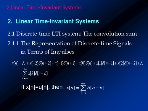
第2章 线性时不变系统
2.1 离散时间LTI系统: 卷积和
(1)用移位单位抽样信号表示离散时间信号 (2)卷积和在离散时间信号LTI系统中的表征 (3)卷积和的计算 (4) 离散时间信号LTI系统的性质
(1)用单位抽样信号表示离散时间信号
x[n] ... x[1] n 1 x[0] n x[1] n 1... x[n][0] x[n 1][1]
(1)初始条件为n<0时,y(n)=0,求其单位抽样响应;
(2)初始条件为n≥0时,y(n)=0,求其单位抽样响应。
解:(1)设x(n) (n),且 y(1) h(1) 0 ,必有
y(n) h(n) 0, n 0
依次迭代
y(0) h(0) (0) 1 y(1) 1 0 1
2
当系统的初始状态为零,单位抽样响应h(n)就 能完全代表系统,那么对于线性时不变系统,任意 输入下的系统输出就可以利用卷积和求得。
差分方程在给定输入和边界条件下,可用迭代 的方法求系统的响应,当输入为δ(n)时,输出 (响应)就是单位抽样响应h(n)。
例:常系数差分方程
y(n) x(n) 1 y(n 1) 2
x[n]u[n] x[k]u[n k] x[k]
k
k
(ii)交换律:
yn xnhn hn xn
例子: 线性时不变系统中的阶跃响应 sn
sn unhn hnun
阶跃输入
输 单位抽样信号 入 响应的累加
n
sn hk
k
(iii)分配律:
xnh1n h2 n xnh1n xnh2 n
y(1) h(1) (1) 1 y(0) 0 1 1
2
22
y(2) h(2) (2) 1 y(1) 0 1 1 (1)2
信号与系统 双语 奥本海姆 第二章PPT课件
10
Chapter 2 §2.3 卷积的计算 1. 由定义计算卷积积分
例2.6 xte au tt,a0htut
2. 图解法 例2.7 求下列两信号的卷积
xt 1 , 0tT ht
0 , 其余t 3. 利用卷积积分的运算性质求解
LTI Systems
yt
t , 0t2T 0 , 其余t
11
Chapter 2
in Terms of impulses
Example 2
3 xn
2
1
1 01 2
n
xknk
x n x 1 n 1 x 0 n x 1 n 1
xnxknk k 4
Chapter 2
LTI Systems
§2.1.2 The Discrete-Time Unit Impulse Responses and the
LTI Systems
§2.3 Properties of LTI Systems
xt ht ytxtht
xn hn ynxnhn
LTI系统的特性可由单位冲激响应完全描述
Example 2.9 ① LTI system
h n
1
0
n0,1 otherwise
② Nonlinear System
③ Time-variant System
a y n x n x n 1 2 aytco s3 txt
b y n m x n ,x a n 1 x b ytetxt 12
Chapter 2
LTI Systems
§2.3.1 Properties of Convolution Integral and Convolution Sum 1. The Commutative Property (交换律)
英文版《信号与系统》第2章讲义
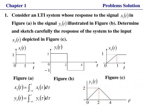
x2 (t ) depicted in Figure (c).
x1 (t )
y1 (t )
x2 (t )
1
0
1
1
1
2 4
t
0
1
t
y2 (t )
2
0
0
1
t
Figure (a)
Figure (b)
Figure (c)
x2 (t ) = ∫ y2 (t ) = ∫
t
∞ t
x1 (τ )dτ y1 (τ )dτ
n = 0,1,2
y(t)
x[n] = {2,1,5}
0
10
Chapter 2
LTI Systems
§2.2 Continuous-Time LTI Systems : The Convolution Integral 卷积积分) (卷积积分) 1. The Representation of Continuous-Time Signals in Terms of impulses
x (t ) = ∫
+∞ ∞
x (τ )δ (t τ )dτ ——Sifting Property
∫
+∞
∞
x(τ )δ (t τ ) dτ = ∫
+∞
∞
x(t )δ (t τ )dτ
+∞ ∞
x(t )δ (t τ )
= x(t )∫
δ (t τ )dτ = x(t )
=1
For example: u(t ) = ∫∞ u(τ )δ (t τ )dτ = ∫0 δ (t τ )dτ
n i =1
LTI Systems
i = 1,2,, n
信号与系统 第二章ppt_part2
1
0 t 1
[1 e(t 1) ]
演示
[1 e(t 1) ]u(t 1) f1 (t ) f2 (t )
f1 (t )* f2 (t )
1
0
1
t
解法二:f 2 ( ) 不变,反褶 f1 ( ), f 2 ( ) f1 ( )
1 1 1
f1 (t ) f2 (t ) f 2 ( ) f1 (t )d
f
( 1) 2
t e d u ( ) e t u (t ) (1 e t )u (t ) (t ) e u ( )d 0
t
f1(t)*f2(t)=(1-e-t) u(t)- [(1-e-(t-2)] u(t-2)
n
即
y zs (t ) lim x(kt )h(t kt )t
t 0 k 0
y zs (t ) lim x(kt )h(t kt )t
t 0 k 0
n
当 t 0 时,t d , kt ,
t 0
t 0
lim
t k 0 0
s(t )
1 e
T
(t T )
e ]u(t T )
t
t
(t T )
]u(t T )
1
0
t
T
演示
例2-13 已知信号x(t)与h(t)如下图所示,求 h(t) x(t) 1 1
y(t ) x(t ) h(t )
-1/2 0 解:
1
t
0
2
t
y (t ) x( )h(t )d
h(t )
1
信号与系统 第二章

( x1 ( t ) + x2 ( t ))* h( t ) = x1 ( t )* h( t ) + x2 ( t )* h( t )
Application: Parallel system a common system Can break a complicated convolution into several simpler ones
Signals & Systems
Example 2.10
1 n x[n] = ( ) u[ n] + 2n u[− n] 2 h[n] = u[n]
Signals & Systems
2.3.3 The Associative Property
x[n]* ( h1 [n]* h2 [n]) = ( x[n]* h1 [n])* h2 [n] x ( t )*[h1 ( t )* h2 ( t )] = [ x ( t )* h1 ( t )]* h2 ( t )
1 h[n] = 0 n = 0,1 otherwise
Example 2.9
If the system is LTI,determine the relationship between input and output If the system is not LTI,determine the relationship between input and output
Signals & Systems
2.2 Continuous-Time LTI System: The Convolution Integral
2.2.1 The Representation ContinuousTime Signals In Term Of Impulse
信号与系统课件(英文)讲解
balance --- y[n] net deposit --- x[n] interest --- 1% so y[n]=y[n-1]+1%y[n-1]+x[n] or y[n]-1.01y[n-1]=x[n]
x[n] Balance in bank y[n]
(sytem
x(t)
t1 y(t)
t2
1 Signal and System
1.6.4 Stability
x[n]
Discrete-time y[n]
System
SISO system
MIMO system?
1 Signal and System
1.5.1 Simple Example of systems
Example 1.8:
RC Circuit in Figure 1.1 : Vc(t) Vs(t)
Memoryless system: It’s output is dependent only on the input at the same time. Features: No capacitor, no conductor, no delayer.
Examples of memoryless system: y(t) = C x(t) or y[n] = C x[n]
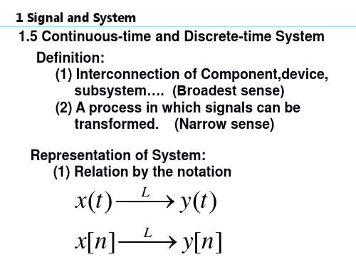
Representation of System: (1) Relation by the notation
x(t) L y(t)
x[n] L y[n]
1 Signal and System
(2) Pictorial Representation
x(t) Continous-time
System
x[n] Balance in bank y[n]
(sytem
x(t)
t1 y(t)
t2
1 Signal and System
1.6.4 Stability
x[n]
Discrete-time y[n]
System
SISO system
MIMO system?
1 Signal and System
1.5.1 Simple Example of systems
Example 1.8:
RC Circuit in Figure 1.1 : Vc(t) Vs(t)
Memoryless system: It’s output is dependent only on the input at the same time. Features: No capacitor, no conductor, no delayer.
Examples of memoryless system: y(t) = C x(t) or y[n] = C x[n]
Representation of System: (1) Relation by the notation
x(t) L y(t)
x[n] L y[n]
1 Signal and System
(2) Pictorial Representation
x(t) Continous-time
System
信号与系统SignalsandSystemsppt课件
0.5
0.4
0.3
0.2
0.1
0
0
1
2
3
4
5
6
7
8
9
10
1
0.9
0.8
0.7
0.6
0.5
0.4
0.3
0.2
0.1
0
0
1
2
3
4
5
6
7
8
9
10
一、基本信号的MATLAB表示
% rectpuls
t=0:0.001:4; T=1; ft=rectpuls(t-2*T,T); plot(t,ft) axis([0,4,-0.5,1.5])
rand
产生(0,1)均匀分布随机数矩阵
randn 产生正态分布随机数矩阵
四、数组
2. 数组的运算
数组和一个标量相加或相乘 例 y=x-1 z=3*x
2个数组的对应元素相乘除 .* ./ 例 z=x.*y
确定数组大小的函数 size(A) 返回值数组A的行数和列数(二维) length(B) 确定数组B的元素个数(一维)
0.3
0.2
0.1
function [f,k]=impseq(k0,k1,k2) 0
-50 -40 -30 -20 -10
0
10 20 30 40 50
%产生 f[k]=delta(k-k0);k1<=k<=k2
k=[k1:k2];f=[(k-k0)==0];
k0=0;k1=-50;k2=50;
[f,k]=impseq(k0,k1,k2);
已知三角波f(t),用MATLAB画出的f(2t)和f(2-2t) 波形
信号与系统奥本海默原版PPT第二章
x(t) h(t)
x(t) h1(t)
x(t)
x(t)*(t)=x(t)
(t)
So, for the invertible system: h(t)*h1(t)=(t) or h[n]*h1[n]=[n]
Example 2.11 2.12
2 Linear Time-Invariant Systems
2.3.6 Causality for LTI system Discrete time system satisfy the condition: h[n]=0 for n<0 Continuous time system satisfy the condition: h(t)=0 for t<0
0, otherwise
We have the expression:
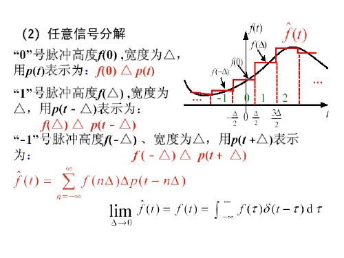
xˆ(t) x(k) (t k)
k
Therefore:
x(t )
lim
0
x(k)
k
(t
k)
2 Linear Time-Invariant Systems
x[n]
y[n]=?
LTI
Solution:
[n] h[n]
[n-k] h[n-k]
x[k][n-k] x[k] h[n-k]
x[n] x[k] [n k] y[n] x[k]h[n k]
k
k
2 Linear Time-Invariant Systems
Memoryless system: Discrete time: y[n]=kx[n], h[n]=k[n] Continuous time: y(t)=kx(t), h(t)=k (t)
- 1、下载文档前请自行甄别文档内容的完整性,平台不提供额外的编辑、内容补充、找答案等附加服务。
- 2、"仅部分预览"的文档,不可在线预览部分如存在完整性等问题,可反馈申请退款(可完整预览的文档不适用该条件!)。
- 3、如文档侵犯您的权益,请联系客服反馈,我们会尽快为您处理(人工客服工作时间:9:00-18:30)。
n
0, n k 0 0, k n h[n k ] 1, n k 0 1, k n
0, k 0 x[k ] u[k ] k , k 0
n
n , x[k ]h[n k ] 0,
0k n otherwise
k 0 k 0
[n k ]
This is identical to the expression we derived in section1.4.
2.1.2 The discrete-time impulse response and the convolution-sum representation of LTI system
(b)
From the figure, we can get
1, n 0,1,2 h[n] 0, otherwise
0.5, n 0 x[n] 2, n 1 0, otherwise
y[n] x[n] h[n]
k
x[k ]h[n k ]
x[1], n 1 x[1] [n 1] 0, n 1
1 n 1 ,the sum of the So ,we can deduce that, for ` three sequences equal to x[n]:
x[n] x[1] [n 1] x[0] [n] x[1] [n 1]
More general, by including additional shifted, scaled impulses, we can write:
x[n] x[1] [n 1] x[0] [n] x[1] [n 1] x[k ] [n k ]
CHAPTER 2 Linear Time-Invariant System
LTI system: A system which is linear and time-invariant is
called LTI system. It is an ideal model of a system, in order to simplify a system for analysis. LTI system play an important role in signal and system analysis. ★First ,many physical processes can be modeled as LTI systems. ★In addition, LTI system can be analyzed in considerable detail, providing both insight into their properties and a set of powerful tools that form the core of signal and a system analysis.
y[n]
k
x[k ]h[n k ]
This result is refer to as the convolution sum ,and the right-hand side of equation is known as the convolution of sequence x[n] and h[n]. We will represent the operation convolution symbolically as
k
Example
Consider an LTI system with impulse h[n] and input x[n], as illustrated in figure (a) and (b), find the response y[n].
(a)
(b)
(a) Solution :
y[1] 0.5h[1] 2h[1 1] 0.5h[1] 2h[0] 0.5 1 2 1 2.5 y[3] 0.5h[3] 2h[3 1] 0.5h[3] 2h[2] 0.5 0 2 1 2.5
Example
Consider an input x[n] and a unit impulse response h[n] given by
From the knowledge we learned in 1.4
x[n] [n n0 ] x[n0 ] [n n0 ]
We can get :
x[1], n -1 x[1] [n 1] n -1 0,
x[0], n 0 x[0] [n] n0 0,
Consider the response of a LTI system to an arbitrary input x[n], if we let h[n k ] denote the response of this system to the shifted unit impulse [n k ] ,then the response of the system to the input x[n] is:
Example
Consider x(t ) u(t ), how to repesentit in termsof impulse?
0 u (t ) 1
0, k n h[n k ] 1, k n
n , x[k ]h[n k ] 0,
0k n otherwise
2.2 Continuous-time LTI system: The convolution integral
2.2.2 The representation of continuous-time signals in terms of impulses
Writing this summation in a more compact form, we have
x[n]
k
x[k ] [n k ]
x[n]
k
x[k ] [n k ]
1 This equation corresponds to the representation of an arbitrary signal as a linear combination of shifted unit impulses [n k ] , where the weights in this linear combination are x[k] 2 This equation is called the sifting property of the discretetime unit impulse. Because the sequence [n k ] is nonzero only when n=k, the summation on the right-hand side “sift” through the sequence values x[k] and preserves only the value corresponding to k=n.
For an arbitrary continuous-time signal x(t), it can be represented as follow:
x(t ) x( ) (t )d
We refer to this equation as the sifting property of the continuous-time impulse.
Example
Consider x[n] u[n], how to repesentit in termsof impulse?
0 x[n] u[n] 1
x[n]
0 k k
n0 n0
x[k ] [n k ] 0 [n k ] 1 [n k ]
n , x[k ]h[n k ] 0,
0k n otherwise
y[n]
k n
x[k ]h[n k ]
for n 0
n 1 1 k 1 k 0
0, n 0 h[n] u[n] 1, n 0
n
0, n 0 h[n] u[n] 1, n 0
0, n 0 x[n] u[n] n , n 0
n
0, n 0 h[n] u[n] 1, n 0
0, n 0 h[n] u[n] 1, n 0
0, n 0 x[n] u[n] n , n 0
x[0]h[n] x[1]h[n 1] 0.5h[n] 2h[n 1]
0 .5
Time shifting
2
y[n] 0.5h[n] 2h[n 1]
y[n] 0.5h[n] 2h[n 1]
y[0] 0.5h[0] 2h[0 1] 0.5 1 2 0 0.5
y[n] x[n] h[n]
y[n]
k
x[k ]h[n k ]
Байду номын сангаас
Note that this equation expresses the response of an LTI system to an arbitrary input in terms of the system’s response to the unit impulse. From this, we see that an LTI system is completely characterized by its response to the unit impulse.