2014 数学建模美赛B题

合集下载

2014 数学建模美赛B题

PROBLEM B: College Coaching LegendsSports Illustrated, a magazine for sports enthusiasts, is looking for the “best all time college coach”male or female for the previous century. Build a mathematical model to choosethe best college coach or coaches (past or present) from among either male or female coaches in such sports as college hockey or field hockey, football, baseball or softball, basketball, or soccer. Does it make a difference which time line horizon that you use in your analysis, i.e., does coaching in 1913 differ from coaching in 2013? Clearly articulate your metrics for assessment. Discuss how your model can be applied in general across both genders and all possible sports. Present your model’s top 5 coaches in each of 3 different sports.In addition to the MCM format and requirements, prepare a 1-2 page article for Sports Illustrated that explains your results and includes a non-technical explanation of your mathematical model that sports fans will understand.问题B：大学教练的故事体育画报，为运动爱好者杂志，正在寻找上个世纪堪称“史上最优秀大学教练”的男性或女性。

2014美赛B数学建模美赛B题数据

2009 2011 1987 1945 1980 1997 1955 1939 1916 1905 1928 2012 1983 1975 1971 1920 1910 1925 1937 1923 1922 1978 1990 1907 1896 1926 1946 1924 1943 1922 1902 1992 1926 1918 1918 1917 1946 1944 1935 1904 1926 1923 1912 1945 1914 1912 1901
Brown Hawaii Fresno State Fordham Towson Stephen F. Austin Murray State Maine Tulsa Oregon State Rochester (NY) Lipscomb Oral Roberts Saint Louis Oklahoma State Georgia Tech St. John's (NY) Kent State Louisville Navy Kentucky Marshall Tennessee State Kansas State Yale DePaul Saint Mary's (CA) Rice Chicago Santa Clara Bloomsburg Sacramento State Utah Virginia Military Institute Muhlenburg Boston University South Carolina Denison Wichita State Brown Valparaiso Rice Roanoke Nevada North Dakota Arizona State Mount Union
names

美国大学生数学建模比赛2014年B题

Team # 26254
Page 2 oon ............................................................................................................................................................. 3 2. The AHP .................................................................................................................................................................. 3 2.1 The hierarchical structure establishment ....................................................................................................... 4 2.2 Constructing the AHP pair-wise comparison matrix...................................................................................... 4 2.3 Calculate the eigenvalues and eigenvectors and check consistency .............................................................. 5 2.4 Calculate the combination weights vector ..................................................................................................... 6 3. Choosing Best All Time Baseball College Coach via AHP and Fuzzy Comprehensive Evaluation ....................... 6 3.1 Factor analysis and hierarchy relation construction....................................................................................... 7 3.2 Fuzzy comprehensive evaluation ................................................................................................................... 8 3.3 calculating the eigenvectors and eigenvalues ................................................................................................ 9 3.3.1 Construct the pair-wise comparison matrix ........................................................................................ 9 3.3.2 Construct the comparison matrix of the alternatives to the criteria hierarchy .................................. 10 3.4 Ranking the coaches .....................................................................................................................................11 4. Evaluate the performance of other two sports coaches, basketball and football.................................................... 13 5. Discuss the generality of the proposed method for Choosing Best All Time College Coach ................................ 14 6. The strengths and weaknesses of the proposed method to solve the problem ....................................................... 14 7. Conclusions ........................................................................................................................................................... 15

2014年美国大学生数学建模MCM-B题O奖论文

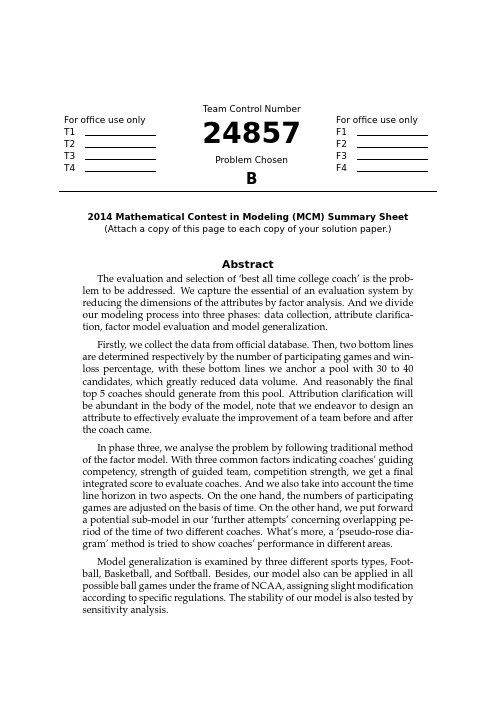
For ofﬁce use only T1T2T3T4T eam Control Number24857Problem ChosenBFor ofﬁce use onlyF1F2F3F42014Mathematical Contest in Modeling(MCM)Summary Sheet (Attach a copy of this page to each copy of your solution paper.)AbstractThe evaluation and selection of‘best all time college coach’is the prob-lem to be addressed.We capture the essential of an evaluation system by reducing the dimensions of the attributes by factor analysis.And we divide our modeling process into three phases:data collection,attribute clariﬁca-tion,factor model evaluation and model generalization.Firstly,we collect the data from ofﬁcial database.Then,two bottom lines are determined respectively by the number of participating games and win-loss percentage,with these bottom lines we anchor a pool with30to40 candidates,which greatly reduced data volume.And reasonably theﬁnal top5coaches should generate from this pool.Attribution clariﬁcation will be abundant in the body of the model,note that we endeavor to design an attribute to effectively evaluate the improvement of a team before and after the coach came.In phase three,we analyse the problem by following traditional method of the factor model.With three common factors indicating coaches’guiding competency,strength of guided team,competition strength,we get aﬁnal integrated score to evaluate coaches.And we also take into account the time line horizon in two aspects.On the one hand,the numbers of participating games are adjusted on the basis of time.On the other hand,we put forward a potential sub-model in our‘further attempts’concerning overlapping pe-riod of the time of two different coaches.What’s more,a‘pseudo-rose dia-gram’method is tried to show coaches’performance in different areas.Model generalization is examined by three different sports types,Foot-ball,Basketball,and Softball.Besides,our model also can be applied in all possible ball games under the frame of NCAA,assigning slight modiﬁcation according to speciﬁc regulations.The stability of our model is also tested by sensitivity analysis.Who’s who in College Coaching Legends—–A generalized Factor Analysis approach2Contents1Introduction41.1Restatement of the problem (4)1.2NCAA Background and its coaches (4)1.3Previous models (4)2Assumptions5 3Analysis of the Problem5 4Theﬁrst round of sample selection6 5Attributes for evaluating coaches86Factor analysis model106.1A brief introduction to factor analysis (10)6.2Steps of Factor analysis by SPSS (12)6.3Result of the model (14)7Model generalization15 8Sensitivity analysis189Strength and Weaknesses199.1Strengths (19)9.2Weaknesses (19)10Further attempts20 Appendices22 Appendix A An article for Sports Illustrated221Introduction1.1Restatement of the problemThe‘best all time college coach’is to be selected by Sports Illustrated,a magazine for sports enthusiasts.This is an open-ended problem—-no limitation in method of performance appraisal,gender,or sports types.The following research points should be noted:•whether the time line horizon that we use in our analysis make a difference;•the metrics for assessment are to be articulated;•discuss how the model can be applied in general across both genders and all possible sports;•we need to present our model’s Top5coaches in each of3different sports.1.2NCAA Background and its coachesNational Collegiate Athletic Association(NCAA),an association of1281institution-s,conferences,organizations,and individuals that organizes the athletic programs of many colleges and universities in the United States and Canada.1In our model,only coaches in NCAA are considered and ranked.So,why evaluate the Coaching performance?As the identity of a college football program is shaped by its head coach.Given their impacts,it’s no wonder high proﬁle athletic departments are shelling out millions of dollars per season for the services of coaches.Nick Saban’s2013total pay was$5,395,852and in the same year Coach K earned$7,233,976in total23.Indeed,every athletic director wants to hire the next legendary coach.1.3Previous modelsTraditionally,evaluation in athletics has been based on the single criterion of wins and losses.Years later,in order to reasonably evaluate coaches,many reseachers have implemented the coaching evaluation model.Such as7criteria proposed by Adams:[1] (1)the coach in the profession,(2)knowledge of and practice of medical aspects of coaching,(3)the coach as a person,(4)the coach as an organizer and administrator,(5) knowledge of the sport,(6)public relations,and(7)application of kinesiological and physiological principles.1Wikipedia:/wiki/National_Collegiate_Athletic_ Association#NCAA_sponsored_sports2USAToday:/sports/college/salaries/ncaaf/coach/ 3USAToday:/sports/college/salaries/ncaab/coach/Such models relatively focused more on some subjective and difﬁcult-to-quantify attributes to evaluate coaches,which is quite hard for sports fans to judge coaches. Therefore,we established an objective and quantiﬁed model to make a list of‘best all time college coach’.2Assumptions•The sample for our model is restricted within the scale of NCAA sports.That is to say,the coaches we discuss refers to those service for NCAA alone;•We do not take into account the talent born varying from one player to another, in this case,we mean the teams’wins or losses purely associate with the coach;•The difference of games between different Divisions in NCAA is ignored;•Take no account of the errors/amendments of the NCAA game records.3Analysis of the ProblemOur main goal is to build and analyze a mathematical model to choose the‘best all time college coach’for the previous century,i.e.from1913to2013.Objectively,it requires numerous attributes to judge and specify whether a coach is‘the best’,while many of the indicators are deemed hard to quantify.However,to put it in theﬁrst place, we consider a‘best coach’is,and supposed to be in line with several basic condition-s,which are the prerequisites.Those prerequisites incorporate attributes such as the number of games the coach has participated ever and the win-loss percentage of the total.For instance,under the conditions that either the number of participating games is below100,or the win-loss percentage is less than0.5,we assume this coach cannot be credited as the‘best’,ignoring his/her other facets.Therefore,an attempt was made to screen out the coaches we want,thus to narrow the range in ourﬁrst stage.At the very beginning,we ignore those whose guiding ses-sions or win-loss percentage is less than a certain level,and then we determine a can-didate pool for‘the best coach’of30-40in scale,according to merely two indicators—-participating games and win-loss percentage.It should be reasonably reliable to draw the top5best coaches from this candidate pool,regardless of any other aspects.One point worth mentioning is that,we take time line horizon as one of the inputs because the number of participating games is changing all the time in the previous century.Hence,it would be unfair to treat this problem by using absolute values, especially for those coaches who lived in the earlier ages when sports were less popular and games were sparse comparatively.4Theﬁrst round of sample selectionCollege Football is theﬁrst item in our research.We obtain data concerning all possible coaches since it was initiated,of which the coaches’tenures,participating games and win-loss percentage etc.are included.As a result,we get a sample of2053in scale.Theﬁrst10candidates’respective information is as below:Table1:Theﬁrst10candidates’information,here Pct means win-loss percentageCoach From To Years Games Wins Losses Ties PctEli Abbott19021902184400.5Earl Abell19281930328141220.536Earl Able1923192421810620.611 George Adams1890189233634200.944Hobbs Adams1940194632742120.185Steve Addazio20112013337201700.541Alex Agase1964197613135508320.378Phil Ahwesh19491949193600.333Jim Aiken19461950550282200.56Fred Akers19751990161861087530.589 ...........................Firstly,we employ Excel to rule out those who begun their coaching career earlier than1913.Next,considering the impact of time line horizon mentioned in the problem statement,we import our raw data into MATLAB,with an attempt to calculate the coaches’average games every year versus time,as delineated in the Figure1below.Figure1:Diagram of the coaches’average sessions every year versus time It can be drawn from theﬁgure above,clearly,that the number of each coach’s average games is related with the participating time.With the passing of time and the increasing popularity of sports,coaches’participating games yearly ascends from8to 12or so,that is,the maximum exceed the minimum for50%around.To further reﬁnethe evaluation method,we make the following adjustment for coaches’participating games,and we deﬁne it as each coach’s adjusted participating games.Gi =max(G i)G mi×G iWhere•G i is each coach’s participating games;•G im is the average participating games yearly in his/her career;and•max(G i)is the max value in previous century as coaches’average participating games yearlySubsequently,we output the adjusted data,and return it to the Excel table.Obviously,directly using all this data would cause our research a mass,and also the economy of description is hard to achieved.Logically,we propose to employ the following method to narrow the sample range.In general,the most essential attributes to evaluate a coach are his/her guiding ex-perience(which can be shown by participating games)and guiding results(shown by win-loss percentage).Fortunately,these two factors are the ones that can be quantiﬁed thus provide feasibility for our modeling.Based on our common sense and select-ed information from sports magazines and associated programs,weﬁnd the winning coaches almost all bear the same characteristics—-at high level in both the partici-pating games and the win-loss percentage.Thus we may arbitrarily enact two bottom line for these two essential attributes,so as to nail down a pool of30to40candidates. Those who do not meet our prerequisites should not be credited as the best in any case.Logically,we expect the model to yield insight into how bottom lines are deter-mined.The matter is,sports types are varying thus the corresponding features are dif-ferent.However,it should be reasonably reliable to the sports fans and commentators’perceptual intuition.Take football as an example,win-loss percentage that exceeds0.75 should be viewed as rather high,and college football coaches of all time who meet this standard are speciﬁcally listed in Wikipedia.4Consequently,we are able toﬁx upon a rational pool of candidate according to those enacted bottom lines and meanwhile, may tender the conditions according to the total scale of the coaches.Still we use Football to further articulate,to determine a pool of candidates for the best coaches,weﬁrst plot theﬁgure below to present the distributions of all the coaches.From theﬁgure2,weﬁnd that once the games number exceeds200or win-loss percentage exceeds0.7,the distribution of the coaches drops signiﬁcantly.We can thus view this group of coaches as outstanding comparatively,meeting the prerequisites to be the best coaches.4Wikipedia:/wiki/List_of_college_football_coaches_ with_a_.750_winning_percentageFigure2:Hist of the football coaches’number of games versus and average games every year versus games and win-loss percentageHence,we nail down the bottom lines for both the games number and the win-loss percentage,that is,0.7for the former and200for the latter.And these two bottom lines are used as the measure for ourﬁrst round selection.After round one,merely35 coaches are qualiﬁed to remain in the pool of candidates.Since it’s theﬁrst round sifting,rather than direct and ultimate determination,we hence believe the subjectivity to some extent in the opt of bottom lines will not cloud theﬁnal results of the best coaches.5Attributes for evaluating coachesThen anchored upon the35candidate selected,we will elaborate our coach evaluation system based on8attributes.In the indicator-select process,we endeavor to examine tradeoffs among the availability for data and difﬁculty for data quantiﬁcation.Coaches’pay,for example,though serves as the measure for coaching evaluation,the corre-sponding data are limited.Situations are similar for attributes such as the number of sportsmen the coach ever cultivated for the higher-level tournaments.Ultimately,we determine the8attributes shown in the table below:Further explanation:•Yrs:guiding years of a coach in his/her whole career•G’:Gi =max(G i)G mi×G i see it at last section•Pct:pct=wins+ties/2wins+losses+ties•SRS:a rating that takes into account average point differential and strength of schedule.The rating is denominated in points above/below average,where zeroTable2:symbols and attributessymbol attributeYrs yearsG’adjusted overall gamesPct win-lose percentageP’Adjusted percentage ratioSRS Simple Rating SystemSOS Strength of ScheduleBlp’adjusted Bowls participatedBlw’adjusted Bowls wonis the average.Note that,the bigger for this value,the stronger for the team performance.•SOS:a rating of strength of schedule.The rating is denominated in points above/below average,where zero is the average.Noted that the bigger for this value,the more powerful for the team’s rival,namely the competition is more ﬁerce.Sports-reference provides ofﬁcial statistics for SRS and SOS.5•P’is a new attribute designed in our model.It is the result of Win-loss in the coach’s whole career divided by the average of win-loss percentage(weighted by the number of games in different colleges the coach ever in).We bear in mind that the function of a great coach is not merely manifested in the pure win-loss percentage of the team,it is even more crucial to consider the improvement of the team’s win-loss record with the coach’s participation,or say,the gap between‘af-ter’and‘before’period of this team.(between‘after’and‘before’the dividing line is the day the coach take ofﬁce)It is because a coach who build a comparative-ly weak team into a much more competitive team would deﬁnitely receive more respect and honor from sports fans.To measure and specify this attribute,we col-lect the key ofﬁcial data from sports-reference,which included the independent win-loss percentage for each candidate and each college time when he/she was in the team and,the weighted average of all time win-loss percentage of all the college teams the coach ever in—-regardless of whether the coach is in the team or not.To articulate this attribute,here goes a simple physical example.Ike Armstrong (placedﬁrst when sorted by alphabetical order),of which the data can be ob-tained from website of sports-reference6.We can easily get the records we need, namely141wins,55losses,15ties,and0.704for win-losses percentage.Fur-ther,speciﬁc wins,losses,ties for the team he ever in(Utab college)can also be gained,respectively they are602,419,30,0.587.Consequently,the P’value of Ike Armstrong should be0.704/0.587=1.199,according to our deﬁnition.•Bowl games is a special event in theﬁeld of Football games.In North America,a bowl game is one of a number of post-season college football games that are5sports-reference:/cfb/coaches/6sports-reference:/cfb/coaches/ike-armstrong-1.htmlprimarily played by teams from the Division I Football Bowl Subdivision.The times for one coach to eparticipate Bowl games are important indicators to eval-uate a coach.However,noted that the total number of Bowl games held each year is changing from year to year,which should be taken into consideration in the model.Other sports events such as NCAA basketball tournament is also ex-panding.For this reason,it is irrational to use the absolute value of the times for entering the Bowl games (or NCAA basketball tournament etc.)and the times for winning as the evaluation measurement.Whereas the development history and regulations for different sports items vary from one to another (actually the differentiation can be fairly large),we here are incapable to ﬁnd a generalized method to eliminate this discrepancy ,instead,in-dependent method for each item provide a way out.Due to the time limitation for our research and the need of model generalization,we here only do root extract of blp and blw to debilitate the differentiation,i.e.Blp =√Blp Blw =√Blw For different sports items,we use the same attributes,except Blp’and Blw’,we may change it according to speciﬁc sports.For instance,we can use CREG (Number of regular season conference championship won)and FF (Number of NCAA Final Four appearance)to replace Blp and Blw in basketball games.With all the attributes determined,we organized data and show them in the table 3:In addition,before forward analysis there is a need to preprocess the data,owing to the diverse dimensions between these indicators.Methods for data preprocessing are a lot,here we adopt standard score (Z score)method.In statistics,the standard score is the (signed)number of standard deviations an observation or datum is above the mean.Thus,a positive standard score represents a datum above the mean,while a negative standard score represents a datum below the mean.It is a dimensionless quantity obtained by subtracting the population mean from an individual raw score and then dividing the difference by the population standard deviation.7The standard score of a raw score x is:z =x −µσIt is easy to complete this process by statistical software SPSS.6Factor analysis model 6.1A brief introduction to factor analysisFactor analysis is a statistical method used to describe variability among observed,correlated variables in terms of a potentially lower number of unobserved variables called factors.For example,it is possible that variations in four observed variables mainly reﬂect the variations in two unobserved variables.Factor analysis searches for 7Wikipedia:/wiki/Standard_scoreTable3:summarized data for best college football coaches’candidatesCoach From To Yrs G’Pct Blp’Blw’P’SRS SOS Ike Armstrong19251949252810.70411 1.199 4.15-4.18 Dana Bible19151946313860.7152 1.73 1.0789.88 1.48 Bernie Bierman19251950242780.71110 1.29514.36 6.29 Red Blaik19341958252940.75900 1.28213.57 2.34 Bobby Bowden19702009405230.74 5.74 4.69 1.10314.25 4.62 Frank Broyles19571976202570.7 3.162 1.18813.29 5.59 Bear Bryant19451982385080.78 5.39 3.87 1.1816.77 6.12 Fritz Crisler19301947182080.76811 1.08317.15 6.67 Bob Devaney19571972162080.806 3.16 2.65 1.25513.13 2.28 Dan Devine19551980222800.742 3.16 2.65 1.22613.61 4.69 Gilmour Dobie19161938222370.70900 1.27.66-2.09 Bobby Dodd19451966222960.713 3.613 1.18414.25 6.6 Vince Dooley19641988253250.715 4.47 2.83 1.09714.537.12 Gus Dorais19221942192320.71910 1.2296-3.21 Pat Dye19741992192400.707 3.16 2.65 1.1929.68 1.51 LaVell Edwards19722000293920.716 4.69 2.65 1.2437.66-0.66 Phillip Fulmer19922008172150.743 3.87 2.83 1.08313.42 4.95 Woody Hayes19511978283290.761 3.32 2.24 1.03117.418.09 Frank Kush19581979222710.764 2.65 2.45 1.238.21-2.07 John McKay19601975162070.7493 2.45 1.05817.298.59 Bob Neyland19261952212860.829 2.65 1.41 1.20815.53 3.17 Tom Osborne19731997253340.8365 3.46 1.18119.7 5.49 Ara Parseghian19561974192250.71 2.24 1.73 1.15317.228.86 Joe Paterno19662011465950.749 6.08 4.9 1.08914.01 5.01 Darrell Royal19541976232970.7494 2.83 1.08916.457.09 Nick Saban19902013182390.748 3.74 2.83 1.12313.41 3.86 Bo Schembechler19631989273460.775 4.12 2.24 1.10414.86 3.37 Francis Schmidt19221942212670.70800 1.1928.490.16 Steve Spurrier19872013243160.733 4.363 1.29313.53 4.64 Bob Stoops19992013152070.804 3.74 2.65 1.11716.66 4.74 Jock Sutherland19191938202550.81221 1.37613.88 1.68 Barry Switzer19731988162090.837 3.61 2.83 1.16320.08 6.63 John Vaught19471973253210.745 4.24 3.16 1.33814.7 5.26 Wallace Wade19231950243070.765 2.24 1.41 1.34913.53 3.15 Bud Wilkinson19471963172220.826 2.83 2.45 1.14717.54 4.94 such joint variations in response to unobserved latent variables.The observed vari-ables are modelled as linear combinations of the potential factors,plus‘error’terms. The information gained about the interdependencies between observed variables can be used later to reduce the set of variables in a putationally this technique is equivalent to low rank approximation of the matrix of observed variables.8 Why carry out factor analyses?If we can summarise a multitude of measure-8Wikipedia:/wiki/Factor_analysisments with a smaller number of factors without losing too much information,we have achieved some economy of description,which is one of the goals of scientiﬁc investi-gation.It is also possible that factor analysis will allow us to test theories involving variables which are hard to measure directly.Finally,at a more prosaic level,factor analysis can help us establish that sets of questionnaire items(observed variables)are in fact all measuring the same underlying factor(perhaps with varying reliability)and so can be combined to form a more reliable measure of that factor.6.2Steps of Factor analysis by SPSSFirst we import the decided datasets of8attributes into SPSS,and the results can be obtained below after the software processing.[2-3]Figure3:Table of total variance explainedFigure4:Scree PlotTheﬁrst table and scree plot shows the eigenvalues and the amount of variance explained by each successive factor.The remaining5factors have small eigenvalues value.Once the top3factors are extracted,it adds up to84.3%,meaning a great as the explanatory ability for the original information.To reﬂect the quantitative analysis of the model,we obtain the following factor loading matrix,actually the loadings are in corresponding to the weight(α1,α2 (i)the set ofx i=αi1f1+αi2f2+...+αim f j+εiAnd the relative strength of the common factors and the original attribute can also be manifested.Figure5:Rotated Component MatrixThen,with Rotated Component Matrix above,weﬁnd the common factor F1main-ly expresses four attributes they are:G,Yrs,P,SRS,and logically,we deﬁne the com-mon factor generated from those four attributes as the guiding competency of the coach;similarly,the common factor F2mainly expresses two attributes,and they are: Pct and Blp,which can be de deﬁned as the integrated strength of the guided team; while the common factor F3,mainly expresses two attributes:SOS and Blw,which can be summarized into a‘latent attribute’named competition strength.In order to obtain the quantitative relation,we get the following Component Score Coefﬁcient Matrix processed by SPSS.Further,the function of common factors and the original attributes is listed as bel-low:F1=0.300x1+0.312x2+0.023x3+0.256x4+0.251x5+0.060x6−0.035x7−0.053x8F2=−0.107x1−0,054x2+0.572x3+0.103x4+0.081x5+0.280x6+0.372x7+0.142x8 F3=−0.076x1−0,098x2−0.349x3+0.004x4+0.027x5−0.656x6+0.160x7+0.400x8 Finally we calculate out the integrated factor scores,which should be the average score weighted by the corresponding proportion of variance contribution of each com-mon factor in the total variance contribution.And the function set should be:F=0.477F1+0.284F2+0.239F3Figure6:Component Score Coefﬁcient Matrix6.3Result of the modelwe rank all the coaches in the candidate pool by integrated score represented by F.Seetable4:Table4:Integrated scores for best college football coach(show15data due to the limi-tation of space)Rank coaches F1F2F3Integrated factor1Joe Paterno 3.178-0.3150.421 1.3622Bobby Bowden 2.51-0.2810.502 1.1113Bear Bryant 2.1420.718-0.142 1.0994Tom Osborne0.623 1.969-0.2390.8205Woody Hayes0.140.009 1.6130.4846Barry Switzer-0.705 2.0360.2470.4037Darrell Royal0.0460.161 1.2680.4018Vince Dooley0.361-0.442 1.3730.3749Bo Schembechler0.4810.1430.3040.32910John Vaught0.6060.748-0.870.26511Steve Spurrier0.5180.326-0.5380.18212Bob Stoops-0.718 1.0850.5230.17113Bud Wilkinson-0.718 1.4130.1050.16514Bobby Dodd0.08-0.2080.7390.16215John McKay-0.9620.228 1.870.151Based on this model,we can make a scientiﬁc rank list for US college football coach-es,the Top5coaches of our model is Joe Paterno,Bobby Bowden,Bear Bryant,TomOsborne,Woody Hayes.In order to conﬁrm our result,we get a ofﬁcial list of bestcollege football coaches from Bleacherreport99Bleacherreport:/articles/890705-college-football-the-top-50-coTable5:The result of our model in football,the last column is ofﬁcial college basketball ranking from bleacherreportRank Our model Integrated scores bleacherreport1Joe Paterno 1.362Bear Bryant2Bobby Bowden 1.111Knute Rockne3Bear Bryant 1.099Tom Osborne4Tom Osborne0.820Joe Paterno5Woody Hayes0.484Bobby Bowden By comparing thoes two ranking list,weﬁnd that four of our Top5coaches ap-peared in the ofﬁcal Top5list,which shows that our model is reasonable and effective.7Model generalizationOur coach evaluation system model,of which the feasibility of generalization is sat-isfying,can be accommodated to any possible NCAA sports concourses by assigning slight modiﬁcation concerning speciﬁc regulations.Besides,this method has nothing to do with the coach’s gender,or say,both male and female coaches can be rationally evaluated by this system.And therefore we would like to generalize this model into softball.Further,we take into account the time line horizon,making corresponding adjust-ment for the indicator of number of participating games so as to stipulate that the evaluation measure for1913and2013would be the same.To further generalize the model,ﬁrst let’s have a test in basketball,of which the data available is adequate enough as football.And the speciﬁc steps are as following:1.Obtain data from sports-reference10and rule out the coaches who begun theircoaching career earlier than1913.2.Calculate each coach’s adjusted number of participating games,and adjust theattribute—-FF(Number of NCAA Final Four appearance).3.Determine the bottom lines for theﬁrst round selection to get a pool of candidatesaccording to the coaches’participating games and win-loss percentage,and the ideal volumn of the pool should be from30to40.Hist diagrams are as below: We determine800as the bottom line for the adjusted participating games and0.7 for the win-loss percentage.Coincidently,we get a candidate pool of35in scale.4.Next,we collect the corresponding data of candidate coaches(P’,SRS,SOS etc.),as presented in the table6:5.Processed by z score method and factor analysis based on the8attributes anddata above,we get three common factors andﬁnal integrated scores.And among 10sports-reference:/cbb/coaches/Figure7:Hist of the basketball coaches’number of games versus and average gamesevery year versus games and win-loss percentagethe top5candidates,Mike Krzyzewski,Adolph Rupp,Dean SmithˇcˇnBob Knightare the same with the ofﬁcial statistics from bleacherreport.11We can say theeffectiveness of the model is pretty good.See table5.We also apply similar approach into college softball.Maybe it is because the popularity of the softball is not that high,the data avail-able is not adequate to employ ourﬁrst model.How can our model function in suchsituation?First and foremost,specialized magazines like Sports Illustrated,its com-mentators there would have more internal and conﬁdential databases,which are notexposed publicly.On the one hand,as long as the data is adequate enough,we can saythe original model is completely feasible.While under the situation that there is datadeﬁcit,we can reasonably simplify the model.The derivation of the softball data is NCAA’s ofﬁcial websites,here we only extractdata from All-Division part.12Softball is a comparatively young sports,hence we may arbitrarily neglect the re-stricted condition of‘100years’.Subsequently,because of the data deﬁcit it is hard toadjust the number of participating games.We may as well determine10as the bottomline for participating games and0.74for win-loss percentage,producing a candidatepool of33in scaleAttributed to the inadequacy of the data for attributes,it is not convenient to furtheruse the factor analysis similarly as the assessment model.Therefore,here we employsolely two of the most important attributes to evaluate a coach and they are:partic-ipating games and win-loss percentage in the coach’s whole career.Speciﬁcally,weﬁrst adopt z score to normalize all the data because of the differentiation of various dimensions,and then the integrated score of the coach can be reached by the weighted11bleacherreport:/articles/1341064-10-greatest-coaches-in-ncaa-b 12NCAA softball Coaching Record:/Docs/stats/SB_Records/2012/coaches.pdf。

2014全国大学生数学建模大赛B题北京赛区

创意平板折叠桌的最优设计摘要本文讨论了某公司的新型产品创意平板折叠桌的设计问题。

从易到难，将问题一步步深化，从各项设计参数已知到客户提出各种需求参数，我们给出最优设计的数学模型。

首先，在平板尺寸、钢筋位置、桌子高度和桌面形状大小均已知的情况下，我们对数据进行计算，给出包括各木条长度、木条开槽长度等的设计加工参数，利用CAD和MATLAB分别绘制出设计图纸及桌角边缘线的四分之一图形。

建立数学模型，通过讨论桌子在不同高度时的状态，给出对创意平板折叠桌动态变化过程的描述。

进而，在仅知桌面高度和桌面形状大小的情况下，我们综合考虑成本、产品稳固性和加工简便性，引入用料体积、临界压力、实际压力、稳定安全因数四个因素，找到其中的最优解，再求出在最优解情况下的开槽长度。

通过对未知的设计参数进行字母设定，以实用和美观为原则，对各项参数给以适当的取值范围，得到平板折叠桌体积的表达式。

由于实际压力不受平板折叠桌结构本身影响，故我们假定一个适当的实际压力值，临界压力和稳定安全因数则由材料力学相关公式给出。

为将成本用料和产品稳固性综合考虑，我们引入稳定安全因数与体积之比这一新的量值，利用Lingo 软件，当其比值最大时，找到了综合考虑成本和产品稳固性的最优解。

在最优解各项设计参数已知后，按照几何关系列式求出相应的开槽长度。

最后，在平板折叠桌的外观要求全部由顾客制定时，我们建立数学模型将平板折叠桌分为三大类，桌面形状分为凸形、凹形和凹凸结合性。

对于每一类，制定不同的平板处理方法，在确定一些满足桌子实用性和美观性基本要求的设计参数的取值范围后，我们给出相应的设计参数最优解的求解步骤。

再利用我们所设计的数学模型结合CAD绘图，给出三种个性设计的创意平板折叠桌的动态变化图示。

关键词：平板折叠桌、最优设计、数学模型、多目标优化、压杆稳定、AutoCAD、MATLAB、Lingo一.问题重述1.1背景某公司生产了一种平板折叠桌，为了增大有效使用面积,设计师以长方形木板的宽为直径截取了一个圆形作为桌面,又将木板剩余的面积切割成了若干个长短不一的木梁,每个木梁的长度为宽到圆上一点的距离,分别用两根全属棒贯穿两侧的木条。

美赛14B题翻译

问题B：大学教练传奇Sports Illustrated, a magazine for sports enthusiasts, is looking for the “best all time college coach” male or female for the previous century. Build a mathematical model to choose the best college coach or coaches (past or present) from among either male or female coaches in such sports as college hockey or field hockey, football, baseball or softball, basketball, or soccer. Does it make a difference which time line horizon that you use in your analysis, i.e., does coaching in 1913 differ from coaching in 2013? Clearly articulate your metrics for assessment. Discuss how your model can be applied in general across both genders and all possible sports. Present your model’s top 5 coaches in each of 3 different sports.体育画报（一个体育爱好者喜爱的杂志）正在评选不限男女上世纪‘最好的全职教练’建立一个数学模型去评选在曲棍球，橄榄球，篮球，垒球，篮球，足球领域里最好的教练（过去或现在）。

2014全国数学建模大赛B题

2014高教社杯全国大学生数学建模竞赛承诺书我们仔细阅读了《全国大学生数学建模竞赛章程》和《全国大学生数学建模竞赛参赛规则》（以下简称为“竞赛章程和参赛规则”，可从全国大学生数学建模竞赛网站下载）。

我们完全明白，在竞赛开始后参赛队员不能以任何方式（包括电话、电子邮件、网上咨询等）与队外的任何人（包括指导教师）研究、讨论与赛题有关的问题。

我们知道，抄袭别人的成果是违反竞赛章程和参赛规则的，如果引用别人的成果或其他公开的资料（包括网上查到的资料），必须按照规定的参考文献的表述方式在正文引用处和参考文献中明确列出。

我们郑重承诺，严格遵守竞赛章程和参赛规则，以保证竞赛的公正、公平性。

如有违反竞赛章程和参赛规则的行为，我们将受到严肃处理。

我们授权全国大学生数学建模竞赛组委会，可将我们的论文以任何形式进行公开展示（包括进行网上公示，在书籍、期刊和其他媒体进行正式或非正式发表等）。

我们参赛选择的题号是（从A/B/C/D中选择一项填写）：我们的参赛报名号为（如果赛区设置报名号的话）：所属学校（请填写完整的全名）：参赛队员(打印并签名)：1.2.指导教师或指导教师组负责人(打印并签名)：（论文纸质版与电子版中的以上信息必须一致，只是电子版中无需签名。

以上内容请仔细核对，提交后将不再允许做任何修改。

如填写错误，论文可能被取消评奖资格。

）赛区评阅编号（由赛区组委会评阅前进行编号）：2014高教社杯全国大学生数学建模竞赛编号专用页赛区评阅编号（由赛区组委会评阅前进行编号）：赛区评阅记录（可供赛区评阅时使用）：评阅人评分备注全国统一编号（由赛区组委会送交全国前编号）：全国评阅编号（由全国组委会评阅前进行编号）：创意平板折叠桌摘要折叠与伸展也已成为家具设计行业普遍应用的一个基本设计理念，占用空间面积小而且家具的功能又更加多样化自然会受到人们的欢迎，着看创意桌子把一整块板分成若干木条，组合在一起，也可以变成很有创意的桌子，就像是变魔术一样，真的是创意无法想象。

2014数学建模b题

对创意平板折叠桌的最优化设计摘要本文主要研究了创意平板折叠桌的相关问题。

对于问题一，首先，我们根据所提供的已知尺寸的长方形平板和桌面形状，桌高的要求，以圆桌面中心作为原点建立了相应的空间直角坐标系，分别求出了各个桌腿的长度，根据在折叠过程中，钢筋穿过的每个点距离桌面的高度相同这一性质，利用MATLAB程序计算出了每根木棒卡槽的长度和桌脚底端每个点的坐标，其中卡槽长度依次为（从最外侧开始，单位：cm）：0、 4.3564、7.663、10.3684、12.5926、14.393、15.8031、16.8445、17.5314、17.8728，并且根据底端坐标拟合出了桌脚边缘线的方程并进行了检验。

另外，我们通过桌脚边缘线的变化图像来描述折叠桌的折叠过程。

对于问题二，我们以用材最少为目标函数，以稳固性好为约束条件，通过对桌腿进行力学分析和几何分析得到了使得用材最少且稳固性好的圆桌需要满足的条件是钢筋穿过最长腿的位置满足一个不等式。

并且，当平板的长为163.4702cm,宽为80cm,厚度为3cm,最外侧桌腿钢筋处到桌腿底端的距离与桌腿的长度之比为0.4186时，木板的用材最小，其对应的体积V为392330cm3。

对于问题三，为了满足客户需求，使得生产的折叠桌尽可能接近客户所期望的形状，我们给出了软件设计的基本算法。

我们考虑了“操场形”桌面和“双曲线形”桌面，得到了“操场形”桌面的的创意平板折叠桌槽长为（从最外侧开始，单位：cm）：0、4.3564、7.6637、10.3684、12.5926、14.3930、15.8031、16.8445、17.5314、17.8728; “曲线形”桌面的创意平板折叠桌槽长为（从最外侧开始，单位：cm）：0、1.5756、2.8917、3.9886、4.9005、5.6532、6.2641、6.7397、7.0741、7.2501。

最后，给出了两种桌面的动态变化图。

关键字：曲线拟合最优化设计几何模型折叠桌桌脚边缘线一、问题重述问题背景某公司生产一种可折叠的桌子，桌面呈圆形，桌腿随着铰链的活动可以平摊成一张平板。

1、下载文档前请自行甄别文档内容的完整性，平台不提供额外的编辑、内容补充、找答案等附加服务。
2、"仅部分预览"的文档,不可在线预览部分如存在完整性等问题,可反馈申请退款(可完整预览的文档不适用该条件!)。
3、如文档侵犯您的权益，请联系客服反馈,我们会尽快为您处理(人工客服工作时间：9:00-18:30)。

PROBLEM B: College Coaching Legends
Sports Illustrated, a magazine for sports enthusiasts, is looking for the “best all time college coach”male or female for the previous century. Build a mathematical model to choose
the best college coach or coaches (past or present) from among either male or female coaches in such sports as college hockey or field hockey, football, baseball or softball, basketball, or soccer. Does it make a difference which time line horizon that you use in your analysis, i.e., does coaching in 1913 differ from coaching in 2013? Clearly articulate your metrics for assessment. Discuss how your model can be applied in general across both genders and all possible sports. Present your model’s top 5 coaches in each of 3 different sports.
In addition to the MCM format and requirements, prepare a 1-2 page article for Sports Illustrated that explains your results and includes a non-technical explanation of your mathematical model that sportsfans will understand.
问题B：大学教练的故事
体育画报，为运动爱好者杂志，正在寻找上个世纪堪称“史上最优秀大学教练”的男性或女性。

建立数学模型，选出在大学曲棍球，足球，棒球或垒球，篮球，橄榄球领域（过去或现在）最好的一个或多个、男性或女性大学教练。

你在你的分析中使用的时间范围对结果有影响吗？比如说，在1913年执教的情况不同于2013年？清楚地说明您的评估指标。

讨论你的模型怎样在男女性别和所有可能的运动中应用。

展示由你的模型得到的3个不同的运动各自排名前5的教练。

除了MCM的格式和要求，准备体育画报一份1-2页的文章，用非技术性的解释向您的体育迷阐述你的结果。

思路：
分析方法多种多样，找平时训练准备的方法模型！数据是关键，看来比较难获得！
层次分析法和模糊评价，主成分分析的精华可以采取，但个人感觉对于美赛这种水平来说不够华丽！重点还需有数据分析做支持！在想点办法排序吧
评价一个教练，可以从执教技术、经验、和管理队员、管理队伍的经验，以及他教出来的运动员成就上评价，还是要把理论数据化！可能会用到模糊数学方面的知识
就美赛而言，查阅获奖论文大多使用智能算法，而且智能算法普遍可以改造分析数据，优化结果！建议搜索相关类型数据分析的文献，用智能算法改造分析，做数据分析支持！结合层次分析
当然尽量进行开放思维和算法的研究，不要局限，美赛注重创新型思维！。

2014 数学建模美赛B题