CONE CRUSHER MODELLING AND SIMULATION
simulation modeling and analysis -回复
simulation modeling and analysis -回复Simulation modeling and analysis is a powerful tool used in various industries to understand complex systems, predict their behavior, and make informed decisions. In this article, we will explore what simulation modeling and analysis are, how they work, and why they are valuable in today's world.Simulation modeling is the process of creating a computer-based representation of a real system or process. It involves developing a mathematical model that captures the key components and interactions of the system. This model is then used to simulate the behavior and performance of the system under different scenarios and conditions.Simulation analysis, on the other hand, refers to the process of evaluating the output or results generated by the simulation model. It involves analyzing and interpreting the data produced during the simulation to gain insights into the system's behavior and performance.The first step in simulation modeling and analysis is defining the objectives and scope of the study. This includes identifying the keyvariables, parameters, and constraints that need to be included in the model. For example, in a manufacturing setting, variables such as production rate, inventory levels, and machine downtime may be of interest.Once the objectives and scope are defined, the next step is data collection. This involves gathering relevant data about the system or process under study. This data can come from a variety of sources, including historical records, surveys, and observations. In some cases, it may be necessary to create synthetic or hypothetical data to supplement the available information.After data collection, the model building phase begins. This involves constructing a mathematical representation of the system using specialized software or programming languages. The model should be able to capture the important characteristics and dynamics of the system, such as its inputs, outputs, and interactions.Next, the model needs to be verified and validated. Verification ensures that the model is free from errors and accurately represents the system. Validation, on the other hand, involvescomparing the output of the model with real-world data or expert knowledge to ensure that it accurately captures the system's behavior.Once the model is verified and validated, the simulation experiments can be conducted. These experiments involve running the model using different input values and scenario conditions to generate data on the system's behavior and performance. The output data can then be analyzed using statistical techniques to understand the effects of various factors on the system's performance.Simulation modeling and analysis provide several benefits. First, they allow decision-makers to experiment with different scenarios and conditions without having to disrupt or modify the real system. This can be particularly valuable in sensitive or high-risk environments, where the consequences of change can be costly or dangerous.Second, simulation modeling and analysis provide a level of detail and visibility that is difficult to achieve through other methods. They allow decision-makers to understand the complexinteractions and dependencies within a system, leading to more informed and effective decision-making.Additionally, simulation modeling and analysis can help optimize system performance. By running multiple simulations and analyzing the results, decision-makers can identify bottlenecks, inefficiencies, and areas of improvement. This can lead to cost savings, increased productivity, and enhanced customer satisfaction.In conclusion, simulation modeling and analysis are valuable tools that enable decision-makers to gain insights into complex systems and make informed decisions. By creating a computer-based representation of a system and running simulations,decision-makers can experiment with different scenarios and conditions to understand the system's behavior and optimize its performance. With the increasing complexity of modern systems, simulation modeling and analysis are becoming essential tools in various industries.。
先进制造技术作业
Concurrent Engineering(并行工程)
一、Concurrent engineering to define and operating characteristics
1.Defined Concurrent engineering products and related processes in parallel, integrated design of a systematic work pattern. This mode of trying to developers from the outset, taking into account the full life cycle of the product of various factors, including quality, cost, schedule and user requirements.
3) Functional integration Various departments functional integration within the enterprise within the product lifecycle and product development collaboration between enterprises and external business functions. 4) Technology Integration Product development involved in the whole process of scientific knowledge and various technical methods of integration, the formation of an integrated knowledge base, method base.
混凝土搅拌车搅拌实验系统仿真设计英文原文

Properties of Fresh ConcreteEdited by H.-J. Wierig Fresh concrete is a mixture of water, cement, aggregate and admixture (if any). After mixing, operations such as transporting, placing, compacting and finishing of fresh concrete can all considerably affect the properties of hardened concrete. It is important that the constituent materials remain uniformly distributed within the concrete mass during the various stages of its handling and that full compaction is achieved. When either of these conditions is not satisfied the properties of the resulting hardened concrete, for example, strength and durability, are adversely affected.The characteristics of fresh concrete which affect full compaction are its consistency, mobility and compactability. In concrete practice these are often collectively known as workability. The ability of concrete to maintain its uniformity is governed by its stability, which depends on its consistency and its cohesiveness. Since the methods employed for conveying, placing and consolidatingd a concrete mix, as well as the nature of the section to be cast, may vary from job to job it follows that the corresponding workability and stability requirements will also vary. The assessment of the suitability of a fresh concrete for a particular job will always to some extent remain a matter of personal judgment.In spite of its importance, the behaviour of plastic concrete often tends to be overlooked. It is recommended that students should learn to appreciate the significance of the various characteristics of concrete in its plastic state and know how these may alter during operations involved in casting a concrete structure.13.1 WorkabilityWorkability of concrete has never been precisely defined. For practical purposes it generally implies the ease with which a concrete mix can be handled from the mixer to its finally compacted shape. The three main characteristics of the property are consistency, mobility and compactability. Consistency is a measure of wetness or fluidity. Mobility defines the ease with which a mix can flow into and completely fill the formwork or mould. Compactability is the ease with which a given mix can be fully compacted, all the trapped air being removed. In this context the required workability of a mix depends not only on the characteristics and relative proportions of the constituent materials but also on (1) the methods employed for conveyance and compaction, (2) the size, shape and surface roughness of formwork or moulds and (3) the quantity and spacing of reinforcement.Another commonly accepted definition of workability is related to the amount of useful internal work necessary to produce full compaction. It should be appreciated that the necessary work again depends on the nature of the section being cast. Measurement of internal work presents many difficulties and several methods have been developed for this purpose but none gives an absolute measure of workability.The tests commonly used for measuring workability do not measure the individual characteristics (consistency, mobility and compactability) of workability. However, they do provide useful and practical guidance on the workability of a mix. Workability affects the quality of concrete and has a direct bearing on cost so that, for example, anunworkable concrete mix requires more time and labour for full compaction. It is most important that a realistic assessment is made of the workability required for given site conditions before any decision is taken regarding suitable concrete mix proportions.13.2 Measurement of WorkabilityThree tests widely used for measuring workability are the slump, compacting factor and V-B consistometer tests (figure 13.1). These are standard tests in the United Kingdom and are described in detail in BS 1881: Part 2. Their use is also recommended in CP 110: Part 1. It is important to note that there is no single relationship between the slump, compacting factor and V-B results for different concretes. In the following sections the salient features of these tests together with their merits and limitations are discussed.Slump TestThis test was developed by Chapman in the United States in 1913. A 300 mm high concrete cone, prepared under standard conditions (BS 1881: Part 2) is allowed to subside and the slump or reduction in height of the cone is taken to be a measure of workability. The apparatus is inexpensive, portable and robustd and is the simplest of all the methods employed for measuring workability. It is not surprising that, in spite of its several limitations, the slump test has retained its popularity.Figure 13.1 Apparatus for workability measurement: (a) slump cone, (b) compacting factor and (c)V-B consistometerThe test primarily measures the consistency of plastic concrete and although it is difficult to see any significant relationship between slump and workability as defined previously, it is suitable for detecting changes in workability. For example, an increase in the water content or deficiency in the proportion of fine aggregate results in anincrease in slump. Although the test is suitable for quality-control purposes it should be remembered that it is generally considered to be unsuitable for mix design since concretes requiring varying amounts of work for compaction can have similar numerical values of slump. The sensitivity and reliability of the test for detecting variation in mixes of different workabilities is largely dependent on its sensitivity to consistency. The test is not suitable for very dry or wet mixes. For very dry mixes, with zero or near-zero slump, moderate variations in workability do not result in measurable changes in slump. For wet mixes, complete collapse of the concrete produces unreliable values of slump.Figure 13.2 Three main types of slumpThe three types of slump usually observed are true slump, shear slump and collapse slump, as illustrated in figure 13.2. A true slump is observed with cohesive and rich mixes for which the slump is generally sensitive to variations in workability. A collapse slump is usually associated with very wet mixes and is generally indicative of poor quality concrete and most frequently results from segregation of its constituent materials. Shear slump occurs more often in leaner mixes than in rich ones and indicates a lack of cohesion which is generally associated with harsh mixes (low mortar content). whenever a shear slump is obtained the test should be repeated and, ifpersistent, this fact should be recorded together with test results, because widely different values of slump can be obtained depending on whether the slump is of true or shear form.The standard slump apparatus is only suitable for concretes in which the maximum aggregate size does not exceed 37.5 mm. It should be noted that the value of slump changes with time after mixing owing to normal hydration processes and evaporation of some of the free water, and it is desirable therefore that tests are performed within a fixed period of time.Compacting Factor TestThis test, developed in the United Kingdom by Glanville et al. (1947), measures the degree of compaction for a standard amount of work and thus offers a direct and reasonably reliable assessment of the workability of concrete as previously defined. The apparatus is a relatively simple mechanical contrivance (figure 13.1) and is fully described in BS 1881: Part 2. The test requires measurement of the weights of the partially and fully compacted concrete and the ratio of the partially compacted weight to the fully compacted weight, which is always less than 1, is known as the compacting factor. For the normal range of concretes the compacting factor lies between 0.80 and 0.92. The test is particularly useful for drier mixes for which the slump test is not satisfactory. The sensitivity of the compacting factor is reduced outside the normal range of workability and is generally unsatisfactory for compacting factors greater than 0.92.It should also be appreciated that, strictly speaking, some of the basic assumptions of the test are not correct. The work done to overcome surface friction of the measuring cylinder probably varies with the characteristics of the mix. It has been shown by Cusens (1956) that for concretes with very low workability the actual work required to obtain full compaction depends on the richness of a mix while the compacting factor remains sensibly unaffected. Thus it follows that the generally held belief that concretes with the same compacting factor require the same amount of work for full compaction cannot always be justified. One further point to note is that the procedure for placing concrete in the measuring cylinder bears no resemblance to methods commonly employed on the site. As in the slump test, the measurement of compacting factor must be made within a certain specified period. The standard apparatus is suitable for concrete with a maximum aggregate size of up to 37.5 mm.V-B Consistometer TestThis test was developed in Sweden by B a hrner (1940) (see figure 13.1). Although generally regarded as a test primarily used in research its potential is now more widely acknowledged in industry and the test is gradually being accepted. In this test (BS 1881: Part 2) the time taken to transform, by means of vibration, a standard cone of concrete to a compacted flat cylindrical mass is recorded. This is known as the V-B time, in seconds, and is stated to the nearest 0.5 s. Unlike the two previous tests, the treatment of concrete in this test is comparable to the method of compacting concrete in practice. Moreover, the test is sensitive to change in consistency, mobility and compactability,and therefore a reasonable correlation between the test results and site assessment of workability can be expected.The test is suitable for a wide range of mixes and, unlike the slump and compacting factor tests, it is sensitive to variations in workability of very dry and also air-entrained concretes. It is also more sensitive to variation in aggregate characteristics such as shape and surface texture. The reproducibility of results is good. As for other tests its accuracy tends to decrease with increasing maximum size of aggregate; above 19.0 mm the test results become somewhat unreliable. For concretes requiring very little vibration for compaction the V-B time is only about 3 s. Such results are likely to be less reliable than for larger V-B times because of the difficulty in estimating the time of the end point (concrete in contact withd the whole of the underside of the plastic disc). At the other end of the workability range, such as with very dry mixes, the recorded V-B times are likely to be in excess of their true workability since prolonged vibration is required to remove the entrapped air bubbles under the transparent disc. To overcome this difficulty an automatic device which records the vertical settlement of the disc with respect to time can be attached to the apparatus. This recording device can also assist in eliminating human error in judging the end point. The apparatus for the V-B test is more expensive than that for the slump and compacting factor tests, requiring an electric power supply and greater experience in handling; all these factors make it more suitable for the precast concrete industry and ready-mixed concrete plants than for general site use.13.3 Factors Affecting WorkabilityVarious factors known to influence the workability of a freshly mixed concrete are shown in figure 13.3. From the following discussion it will be apparent that a change in workability associated with the constituent materials is mainly affected by water content and specific surface of cement and aggregate.Cement and WaterFigure 13.3 Factors affecting workability of fresh conreteTypical relationships between the cement-water ratio (by volume) and the volume fraction of cement for different workabilities are shown in figure 15.5. The change in workability for a given change in cement-water ratio is greater when the water content is changed than when only the cement content is changed. In general the effect of the cement content is greater for richer mixes. Hughes (1971) has shown that similar linear relationships exist irrespective of the properties of the constituent materials.For a given mix, the workability of the concrete decreases as the fineness of the cement increases as a result of the increased specific surface, this effect being more marked in rich mixtures. It should also be noted that the finer cements improve the cohesiveness of a mix. With the exception of gypsum, the composition of cement has no apparent effect on workability. Unstable gypsum is responsible for false set, which can impair workability unless prolonged mixing or remixing of the fresh concrete is carriedout. Variations in quality of water suitable for making concrete have no significant effect on workability.AdmixturesThe principal admixtures affecting improvement in the workability of concrete are water-reducing and air-entraining agents. The extent of the increase in workability is dependent on the type and amount of admixture used and the general characteristics of the fresh concrete.Workability admixtures are used to increase workability while the mix proportions are kept constant or to reduce the water content while maintaining constant workability. The former results in a slight reduction in concrete strength.Air-entraining agents are by far the most commonly used workability admixtures because they also improve both the cohesiveness of the plastic concrete and the frost resistance of the resulting hardened concrete. Two points of practical importance concerning air-entrained concrete are that for a given amount of entrained air, the increase in workability tends to be smaller for concretes containing rounded aggregates or low cement-water ratios (by volume) and, in general, the rate of increase in workability tends to decrease with increasing air content. However, as a guide it may be assumed that every 1 per cent increase in air content will increase the compacting factor by 0.01 and reduce the V-B time by 10 per cent.AggregateFor given cement, water and aggregate contents, the workability of concrete is mainly influenced by the total surface area of the aggregate. The surface area is governed by the maximum size, grading and shape of the aggregate. Workability decreases as the specific surface increases, since this requires a greater proportion of cement paste to wet the aggregate particles, thus leaving a smaller amount of paste for lubrication. It follows that, all other conditions being equal, the workability will be increased when the maximum size of aggregate increases, the aggregate particles become rounded or the overall grading becomes coarser. However, the magnitude of this change in workability depends on the mix proportions, the effect of the aggregate being negligible for very rich mixes (aggregate-cement ratios approaching 2). The practical significance of this is that for a given workability and cement-water ratio the amount of aggregate which can be used in a mix varies depending on the shape, maximum size and grading of the aggregate, as shown in figure 13.4 and tables 13.1 and 13.2. The influence of air-entrainment (4.5 per cent) on workability is shown also in figure 13.4.TABLE 13.1Effect of maximum size of aggregate of similar grading zone on aggregate-cement ratio of concrete having water-cement ratio of 0.55 by weight, based on McIntosh (1964)Maximum aggregatesize(mm)Aggregate-cement ratio (by weight)Low workability Medium workability High workability IrregulargravelCrushed rockIrregulargravelCrushed rockIrregulargravelCrushed rock9.5 5.3 4.8 4.7 4.2 4.4 3.719.0 37.56.27.65.56.45.46.54.75.54.95.94.45.2TABLE 13.2Effect of aggregate grading (maximum size 19.0 mm) on aggregate-cement ratio ofconcrete having medium workability and water-cement ratio of 0.55 by weight, based onMcIntosh (1964)Type of aggregateAggregate-cement ratioCoarse grading Fine gradingRounded gravel Irregular gravel Crushed rock 7.35.54.76.35.14.3Figure 13.4 Effect of aggregate shape on aggregate-cement ratio of concretes for different workabilities, based on Cornelius (1970)Several methods have been developed for evaluating the shape of aggregate, asubject discussed in chapter 12. Angularity factors together with grading modulus and equivalent mean diameter provide a means of considering the respective effects of shape, size and grading of aggregate (see chapter 15). Since the strength of a fully compacted concrete, for given materials and cement-water ratio, is not dependent on the ratio of coarse to fine aggregate, maximum economy can be obtained by using the coarse aggregate content producing the maximum workability for a given cement content (Hughes, 1960) (see figure 13.5). The use of optimum coarse aggregate content in concrete mix design is described in chapter 15. It should be noted that it is the volume fraction of an aggregate, rather than its weight, which is important.Figure 13.5 A typical relationship between workability and coarse aggregate content of concrete, based on Hughes (1960)The effect of surface texture on workability is shown in figure 13.6. It can be seen that aggregates with a smooth texture result in higher workabilities than aggregates with a rough texture. Absorption characteristics of aggregate also affect workability where dry or partially dry aggregates are used. In such a case workability drops, the extent of the reduction being dependent on the aggregate content and its absorption capacity.Ambient ConditionsEnvironmental factors that may cause a reduction in workability are temperature, humidity and wind velocityd. For a given concrete, changes in workability are governed by the rate of hydration of the cement and the rate of evaporation of water. Therefore both the time interval from the commencement of mixing to compaction and the conditions of exposure influence the reduction in workability. An increase in the temperature speeds up the rate at which water is used for hydration as well as its loss through evaporation. Likewise wind velocity and humidity influence the workability as they affect the rate of evaporation. It is worth remembering that in practice these factors depend on weather conditions and cannot be controlled.Figure 13.6 Effect of aggregate surface texture on aggregate-cement ratio of concretes for different workabilities, based on Cornelius (1970)TimeThe time that elapses between mixing of concrete and its final compaction depends onthe general conditions of work such as the distance between the mixer and the point of placing, site procedures and general management. The associated reduction in workability is a direct result of loss of free water with time through evaporation, aggregate absorption and initial hydration of the cement. The rate of loss of workability is affected by certain characteristics of the constituent materials, for example, hydration and heat development characteristics of the cement, initial moisture content and porosity of the aggregate, as well as the ambient conditions.For a given concrete and set of ambient conditions, the rate of loss of workability with time depends on the conditions of handling. Where concrete remains undisturbed after mixing until it is placed, the loss of workability during the first hour can be substantial, the rate of loss of workability decreasing with time as illustrated by curve A in figure 13.7. On the other hand, if it is continuously agitated, as in the case of ready-mixed concrete, the loss of workability is reduced, particularly during the first hour or so (see curve B in figure 13.7). However, prolonged agitation during transportation may increase the fineness of the solid particles through abrasion and produce a further reduction in workability. For concretes continuously agitated and undisturbed during transportation, the time intervals permitted (BS 1926) between the commencement of mixing and delivery on site are 2 hours and 1 hour respectively.For practical purposes, loss of workability assumes importance when concrete becomes so unworkable that it cannot be effectively compacted, with the result that its strength and other properties become adversely affected. Corrective measures frequently taken to ensure that concrete at the time of placing has the desired workability are eitheran initial increase in the water content or an increase in the water content with further mixing shortly before the concrete is discharged. When this results in a water content greater than that originally intended, some reduction in strength and durability of the hardened concrete is to be expected unless the cement content is increased accordingly. This important fact is frequently overlooked on site. It should be recalled that the loss of workability varies with the mix, the ambient conditions, the handling conditions and the delivery time. No restriction on delivery time is given in CP 110: Part 1 but the concrete must be capable of being placed and effectively compacted without the addition of further water. For detailed information on the use of ready-mixed concrete the reader is advised to consult the work of Dewar (1973).Figure 13.7 Loss of workability of concrete with time: (A) no agitation and (B)continuously agitated after mixing13.4 StabilityApart from being sufficiently workable, fresh concrete should have a composition such that its constituent materials remain uniformly distributed in the concrete during both the period between mixing and compaction and the period following compaction beforethe concrete stiffens. Because of differences in the particle size and specific gravities of the constituent materials there exists a natural tendency for them to separate. Concrete capable of maintaining the required uniformity is said to be stable and most cohesive mixes belong to this category. For an unstable mix the extent to which the constituent materials will separate depends on the methods of transportation, placing and compaction. The two most common features of an unstable concrete are segregation and bleeding.SegregationWhen there is a significant tendency for the large and fine particles in a mix to become separated, segregation is said to have occurred. In general, the less cohesive the mix the greater the tendency for segregation to occur. Segregation is governed by the total specific surface of the solid particles including cement and the quantity of mortar in the mix. Harsh, extremely wet and dry mixes as well as those deficient in sand, particularly the finer particles, are prone to segregation. As far as possible, conditions conducive to segregation such as jolting of concrete during transportation, dropping from excessive heights during placing and over-vibration during compaction should be avoided.Blemishes, sand streaks, porous layers and honeycombing are a direct result of segregation. These features are not only unsightly but also adversely affect strength, durability and other properties of the hardened concrete. It is important to realize that the effects of segregation may not be indicated by the routine strength tests on control specimens since the conditions of placing and compaction of the specimens differ fromthose in the actual structure. There are no specific rules for suspecting possible segregation but after some experience of mixing and handling concrete it is not difficult to recognize mixes where this is likely to occur. For example, if a handful of concrete is squeezed in the hand and then released so that it lies in the palm, a cohesive concrete will be seen to retain its shape. A concrete which does not retain its shape under these conditions may well be prone to segregation and this is particularly so far wet mixes.BleedingDuring compaction and until the cement paste has hardened there is a natural tendency for the solid particles, depending on size and specific gravity, to exhibit a downward movement. Where the consistency of a mix is such that it is unable to hold all its water some of it is gradually displaced and rises to the surface, and some may also leak through the joints of the formwork. Separation of water from a mix in this manner is known as bleeding. While some of the water reaches the top surface some may become trapped under the larger particles and under the reinforcing bars. The resulting variations in the effective water content within a concrete mass produce corresponding changes in its properties. For example, the strength of the concrete immediately underneath the reinforcing bars and coarse aggregate particles may be much less than the average strength and the resistance to percolation of water in these areas is reduced. In general, the concrete strength tends to increase with depth below the top surface. The water which reaches the top surface presents the most serious practical problems. If it is not removed, the concrete at and near the top surface will be much weaker andless durable than the remainder of the concrete. This can be particularly troublesome in slabs which have a large surface area. On the other hand, removal of the surface water will unduly delay the finishing operation on the site.The risk of bleeding increases when concrete is compacted by vibration although this may be minimized by using a correctly designed mix and ensuring that the concrete is not over-vibrated. Rich mixes tend to bleed less than lean mixes. The type of cement employed is also important, the tendency for bleeding to occur decreasing as the fineness of the cement or its alkaline and tricalcium aluminate (C3A) content increases. Air-entrainment provides another very effective means of controlling bleeding in, for example, wet lean mixes where both segregation and bleeding are frequently troublesome.。
Geometric Modeling
Geometric ModelingGeometric modeling is a fundamental concept in the field of computer graphics, design, and engineering. It involves the creation of digital representations of objects and environments using mathematical and computational techniques. This process is essential for various applications, including animation, virtual reality, architectural design, and manufacturing. In this response, we willexplore the historical background, different perspectives, case studies, and a critical evaluation of geometric modeling, as well as its future implications and recommendations. The development of geometric modeling can be traced back to the early 1960s when Ivan Sutherland created Sketchpad, one of the first computer-aided design (CAD) programs. This revolutionary software allowed users to interactively manipulate geometric shapes on a computer screen, laying the foundation for modern geometric modeling techniques. Over the years, advancementsin computer hardware and software have led to the development of moresophisticated modeling tools, such as parametric modeling, solid modeling, and surface modeling. These tools have greatly improved the efficiency and accuracy of design and engineering processes, making geometric modeling an indispensable part of various industries. From a historical perspective, geometric modeling has evolved from simple wireframe models to complex three-dimensional (3D) representations that accurately simulate real-world objects. This evolution has been driven by the increasing demand for realistic visualizations in fields suchas entertainment, gaming, and virtual reality. Additionally, the integration of geometric modeling with computer-aided manufacturing (CAM) has revolutionized the production of physical objects, allowing for the creation of intricate and precise designs that were previously unattainable. From a practical standpoint, geometric modeling has become an indispensable tool for architects, engineers, and designers. For example, in architectural design, 3D modeling software allows architects to create detailed digital models of buildings, enabling them to visualize and modify designs before construction. Similarly, in product design and manufacturing, geometric modeling facilitates the creation of prototypes and production-ready models, streamlining the entire product development process. These examples demonstrate the widespread impact of geometric modeling on various industries andits role in driving innovation and efficiency. Despite its numerous benefits, geometric modeling also presents certain challenges and limitations. One of the primary drawbacks is the complexity of creating and manipulating 3D models, which often requires specialized skills and training. This can be a barrier for individuals and organizations that lack the resources to invest in training and software. Furthermore, the accuracy and precision of geometric models heavily rely on the quality of input data and the algorithms used, which can introduce errors and discrepancies in the final output. Additionally, the computational resources required for complex geometric modeling tasks can be substantial, posing a challenge for users with limited hardware capabilities. To illustrate the practical implications of geometric modeling, let us consider a case study in the automotive industry. Car manufacturers utilize 3D modeling software to design and visualize new vehicle models, enabling them to iterate on designs and evaluate aesthetic and functional aspects before production. This process not only reduces the time and cost of prototyping but also allows for the exploration of innovative and ergonomic designs that enhance the overall driving experience. Furthermore, geometric modeling plays a crucial role in simulating crash tests and aerodynamic analyses, ensuring the safety and performance of vehicles. In conclusion, geometric modeling is a vital component of modern design, engineering, and manufacturing processes, offering numerous benefits while also presenting challenges. Its historical development has been marked by significant advancements in software and hardware technology, leading to its widespread adoption across various industries. While the complexity and resource requirements of geometric modeling pose challenges, its practical implications are evident in fields such as architecture, product design, and automotive engineering. Looking ahead, the continued evolution of geometric modeling tools and techniques is expected to further enhance its capabilities and accessibility, paving the way for new applications and innovations. As such, it is crucial for individuals and organizations to stay abreast of these developments and invest in the necessary skills and resources to leverage the full potential of geometric modeling.。
simulation modelling practice -回复
simulation modelling practice -回复Simulation Modelling Practice: A Step-by-Step GuideIntroduction:Simulation modelling is a valuable technique used to mimicreal-life systems and analyze their behavior. By creating virtual representations of complex systems, simulation modelling allows us to understand how different variables and factors interact and impact the overall system performance. In this article, we will provide a step-by-step guide on how to develop and execute a simulation model, ensuring accurate results and valuable insights.Step 1: Define the Scope and ObjectivesThe first and most crucial step in simulation modelling is to clearly define the scope and objectives of the study. This involves understanding the problem at hand, identifying the variables to be considered, and determining the specific goals to be achieved. For instance, if you are simulating a supply chain network, clarify whether you aim to optimize inventory levels, reduce lead time, or minimize costs.Step 2: Gather DataSimulating a system requires accurate and comprehensive data. Collecting data from reliable sources is essential to ensure the validity and reliability of the simulation model. This could include historical data, market trends, customer demand data, and any other relevant information. Data can be obtained through surveys, interviews, observations, or existing databases.Step 3: Develop the Conceptual ModelOnce the data is gathered, the next step is to develop the conceptual model. This involves identifying the components, relationships, and behaviors of the system to be simulated. Conceptual models can be represented using flowcharts, diagrams, or mathematical equations, depending on the complexity of the system.Step 4: Convert the Conceptual Model into a Computer ModelIn this step, the conceptual model is translated into a computer model using specialized simulation software. Multiple software options are available, such as AnyLogic, Simul8, or Arena. The choice of software depends on factors like complexity, desired output, and personal preference. The computer model includes allthe variables, parameters, and rules defined in the conceptual model.Step 5: Validate the ModelModel validation is crucial for ensuring the accuracy and reliability of simulation results. This involves comparing the model's output to real-life data or expert opinions. Validation can be done by running the simulation model on past data and evaluating how well it replicates the actual outcomes. If the model does not produce results that align with reality, adjustments are made until satisfactory validation is achieved.Step 6: Design Experiments and Run SimulationsBefore running simulations, it is important to design experiments that address the objectives defined in Step 1. Experiment design includes specifying the values for each variable, defining replication and randomization strategies, and determining the desired performance measures to be analyzed. Once the experiments are designed, simulations are executed using the computer model, and data is collected for subsequent analysis.Step 7: Analyze ResultsSimulation outputs provide valuable insights into system behavior. This step involves analyzing the simulation results to gain a deeper understanding of the system's performance. Statistical techniques like regression analysis, variance analysis, or Monte Carlo simulation can be used to explore the relationship between variables, identify performance bottlenecks, and optimize system performance.Step 8: Implement ImprovementsBased on the insights gained from the simulation analysis, improvements can be implemented to optimize the system. These improvements could involve adjusting parameters, redesigning processes, or reallocating resources. By simulating the effects of these changes, decision-makers can evaluate their impact on system performance and make informed decisions.Step 9: Communicate FindingsThe final step involves effectively communicating the findings and recommendations derived from the simulation study. Visualizations, such as charts, graphs, or interactive dashboards, can be used to present the results in a clear and concise format. This helps stakeholders understand the implications of the analysis andsupports informed decision-making.Conclusion:Simulation modelling is a powerful tool that allows us to study and optimize complex systems. By following the step-by-step guide outlined in this article, practitioners can develop reliable and insightful simulation models. Remember to define the scope and objectives, gather accurate data, design a conceptual model, convert it into a computer model, validate the model's outputs, run simulations, analyze the results, implement improvements, and effectively communicate the findings. By systematically going through these steps, you can unlock the potential of simulation modelling to tackle complex problems and drive informed decision-making.。
颚式破碎机的建模与仿真分析
毕业设计题目颚式破碎机的建模与仿真分析英文题目 Modeling and Simulation Analysis ofJaw Crusher院系机械与材料工程学院专业机械设计制造及其自动化姓名年级指导教师二零一五年六月摘要Pro/E是三维参数化设计软件,常用于机械、电子、汽车制造、航空航天等重要领域。
本文运用Pro/E软件完成了颚式破碎机的三维建模设计与仿真,其中利用Pro/E的草绘模块,零件模块共同完成了颚式破碎机四个组成部件的建模设计,并对其进行仿真。
同时利用Pro/E的组建模块完成了组成部分的装配和干涉检验。
通过对各个部分零件的设计,证明Pro/E软件在进行复杂的典型产品开发过程中具有简单,方便,快捷的特点。
国内的颚式破碎机类型很多,但常见的还是复摆颚式破碎机。
复摆颚式破碎机经过人们长期的实践和不断完善与改进,其结构型式和机构参数日臻合理,因此在很多行业使用非常广泛。
随着现代化的发展,各工业部门对破碎石的需求进一步增长,研究复摆颚式破碎机具有很重要的意义。
【关键词】颚式破碎机;Pro/E;三维建模设计;运动仿真AbstractPro/E is 3D parametric design software and it commonly used in machinery ,electronics, automobile ,manufacturing, aerospace and other field. In this paper, the three-dimensional design of jaw crusher was design by the software of Pro/E. The design of four modeling was completed by the Sketch of the module , and make a simulation analysis for the jaw crusher. the design of the component proved that Pro/E software is simple , convenient ,and fast in a typical complex product development process.There are many kinds of Jaw-fashioned Crusher in China, But common traditional type is compound pendulum jaw crusher . And consummates and the improvement unceasingly after the people long-term practice, Its structure pattern and the organization parameter are reasonable, The structure simple, , therefore ,it was used in many field ,which is extremely widespread. Along with the modernized development, various industry sector further grows to the broken crushed stone demand, studies the duplicate pendulum Jaw-fashioned Crusher to have the vital significance.【Key words】Jaw Crusher ;Pro/E;Three-dimensional design ;Motion simulation目录前言 (5)第一章绪论 (7)1.1 Pro/E的简介 (7)1.2 Pro/E模块介绍 (7)1.3 Pro/E工作界面 (9)第二章颚式破碎机 (11)2.1 研究的目的和意义 (11)2.2 复摆颚式破碎机特点 (13)2.3 基本结构和工作原理 (15)2.3.1 颚式破碎机基本结构 (15)2.3.2 破碎机工作原理 (15)第三章颚式破碎机三维造型 (16)3.1 连杆的三维造型 (16)3.2 曲柄的三维造型 (20)3.3 机架的三维造型 (25)3.4 机架的三维造型 (29)第四章破碎机的装配和仿真运动 (31)4.1 破碎机的装配 (31)4.2 破碎机的仿真 (36)4.2.1 仿真运动的参数设置 (36)4.2.1 颚式破碎机仿真运动效果 (38)4.2.3 颚式破碎机仿真运动分析 (40)结论 (45)参考文献 (46)谢词 (48)前言在我国基础建设工程中,需要大量的,各种不同粒径的砂、石作为生产之用。
Simulation and conparision of three technologies
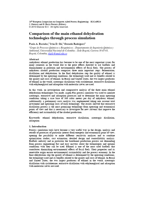
20th European Symposium on Computer Aided Process Engineering – ESCAPE20S. Pierucci and G. Buzzi Ferraris (Editors)© 2010 Elsevier B.V. All rights reserved.Comparison of the main ethanol dehydration technologies through process simulationPaola A. Bastidas,a Iván D. Gil,a Gerardo Rodríguez aa Grupo de Procesos Químicos y Bioquímicos – Departamento de Ingeniería Química y Ambiental, Universidad Nacional de Colombia – Sede Bogotá, Carrera 30 45-03,Bogotá, Colombia, idgilc@.coAbstractAnhydrous ethanol production has become to be one of the most important issues for many countries in the world due to the great efforts directed to use biofuels and diminishment in pollution and environmental effects of fossil fuels. The process of anhydrous alcohol production comprises three main important steps: fermentation, distillation and dehydration. In the final dehydration step the quality of ethanol is determined by the operating conditions, the technology used and its benefits related to the quality and costs of ethanol. In Brazil and United States, the two largest producers of ethanol in the world, azeotropic distillation with cyclohexane, extractive distillation with ethyleneglycol and adsorption with molecular sieves are used.In this work, an investigation and comparative analysis of the three main ethanol dehydration technologies was made. Aspen Plus process simulator was used to simulate azeotropic, extractive and adsorption processes and to determine the main operating conditions taking a case base of 300 cubic meters per day of anhydrous ethanol. Additionally, a preliminary costs analysis was implemented taking into account total investment and operating costs of each technology. The results showed that extractive distillation process is the most promising technology from operating and economical points of view and that is necessary to investigate for new solvents that improve the efficiency and sustainability of the alcohol production.Keywords: ethanol dehydration, extractive distillation, azeotropic distillation, adsorption1.IntroductionProcess simulation tools have become a very useful way in the design, analysis and retrofit of processes of particular interest from energetic and economical point of view, opening the possibility to make different sensitivity analyses and to combine optimization studies, cost estimation, detailed design and controllability analysis. Biofuels industry and in particular the bioethanol production process are demanding from process engineering fast and easy answers about the technologies and optimal conditions with they can be used. Ethanol is one of the most used biofuels that contributes diminishing environmental effects of fossil fuels. Their properties and its renewable origin ensure environmental sustainability and the process economy. In the final dehydration step the quality of ethanol is determined by the operating conditions, the technology used and its benefits related to the quality and costs of ethanol. In Brazil and United States, the two largest producers of ethanol in the world, azeotropic distillation with cyclohexane, extractive distillation with ethyleneglycol and adsorption with molecular sieves are used.P. Bastidas et al. Heterogeneous azeotropic distillation has been widely studied in many papers and textbooks and widely applied in alcohol industry to dehydrate ethanol (e.g. 60% of dehydration plants in Brazil are azeotropic distillation based). However, heterogeneous azeotropic distillation reports some disadvantages associated with the high degree of nonlinearity, multiple steady states, distillation boundaries, long transients, and heterogeneous liquid-liquid equilibrium, limiting the operating range of the system under different feed disturbances [1-5]. Extractive distillation is based on the introduction of a selective solvent that interacts differently with each of the components of the mixture and mainly shows affinity with one of the key components [3, 6]. The principle driving extractive distillation is based on the introduction of a selective solvent that interacts differently with each of the components of the original mixture and which generally shows a strong affinity with one of the key components [4, 7, 8]. Adsorption on molecular sieves takes advantage of the difference of molecular size of ethanol and water molecules to adsorb in a selective way water molecules and allowing ethanol separation. Molecular sieves are materials composed by microporous substances that are characterized by their excellent ability to retain on its surface defined types of chemical species. These materials packed into a vessel make possible to separate ethanol from ethanol-water mixtures by adsorption mechanisms at high pressure.In this work the three main ethanol dehydration technologies will be studied in order to establish the main operating conditions required to obtain high purity ethanol. Rigorous simulations in Aspen Plus for a plant producing 300 cubic meters per day of anhydrous ethanol will be carried out and some economical considerations are included in the comparison of the technologies available.2.Process SimulationEthanol-water mixture at atmospheric pressure has a minimum-boiling homogeneous azeotrope at 78.1°C of composition 89 mol% ethanol. The NRTL physical property model is used to describe the nonideality of the liquid phase and the vapor is assumed to be ideal. All NRTL model binary parameters are taken from Aspen Plus database. For all of the three processes simulated azeotropic ethanol was the feed and anhydrous ethanol with purity higher than 99.5 mole % was fixed as the main product. On the next subsections are described briefly each one of the processes and the main operating conditions established are reported.2.1.Azeotropic distillation with cyclohexaneAzeotropic distillation uses a solvent with an intermediate boiling point to introduce new azeotropes to the mixture and at the same time to generate two liquid phases that allow, in a combined way, separating ethanol from water. This technique although is widely used has lost acceptance due to its poor stability and high energy consumption. The process flowsheet of azeotropic distillation is shown on Fig. 1. The process has two columns and one decanter. The first heterogeneous azeotropic distillation column is designed to obtain high-purity ethanol product at the column bottom while obtaining minimum boiling ethanol-water-cyclohexane azeotrope at the top of the column. The azeotrope obtained at the top is heterogeneous and the top vapor stream is then condensed to form two liquid phases in the decanter [7, 9]. The organic phase containing mainly cyclohexane is refluxed back to the heterogeneous azeotropic distillation column. The aqueous phase is drawn out from the decanter to be sent to the entrainer recovery column where at the bottoms stream is obtained water essentially pure and at the top is removed cyclohexane to be recycled to the first column.Comparison of the main ethanol dehydration technologies through process simulationMakeupCyclohexaneFigure 1. Flowsheet for azeotropic distillation with cyclohexaneThe results obtained show that is possible to produce anhydrous ethanol using cyclohexane as entrainer with high mole recovery of ethanol. As the top vapor concentration approaches to the ternary heterogeneous azeotrope, the separation is achieved is improved in the dehydration column. As the organic reflux flow rate and the recycle flow rate increase the ethanol concentration at the bottoms of the dehydration column also increase improving the separation performance but also increasing the heat duties. The operating conditions are used to calculate the hydraulic performance and to estimate the column diameters, information useful to calculate the capital costs.2.2.Extractive distillation with ethyleneglycolExtractive distillation is a partial vaporization process in the presence of a non-volatile and high boiling point entrainer which does not form any azeotropes with the original components of the azeotropic mixture. The process flowsheet of extractive distillation system is presented on Fig. 2. The process has two columns: the extractive distillation column and the entrainer recovery column. The entrainer is continuously fed in one of the top stages of the extractive column while the azeotropic feed is entered in a middle stage lower down the column. At the top of the extractive distillation column is obtained anhydrous ethanol and at the bottoms stream is removed a mixture of water-ethyleneglycol which is send to the second entrainer recovery column. In the recovery column at the top water is withdrawn with some traces of ethanol and at the bottom high-purity ethyleneglycol is recycled back to the extractive distillation column [9].Extractive distillation process with ethyleneglycol show some important advantages respect to azeotropic ones. The makeup entrainer is much lower than azeotropic case and additionally the quantity of entrainer is lower which affect the diameter of the columns. It can be observed that the column diameters are smaller in the extractive distillation systems and also the energy consumption in the columns. On the other hand,P. Bastidas et al. the most important variables used to achieve the desired ethanol concentration are the entrainer to feed molar ratio and the reflux ratio. The former has a little effect over the energy consumption compared with the reflux ratio impact on the reboiler duty, for this reason the reflux ratio in extractive distillation column is fixed at the best low value.MakeupEthGlycolReboiler Duty4316.82 kWReboiler Duty566.88 kWFigure 2. Flowsheet for extractive distillation with ethyleneglycol2.3.Adsorption with molecular sievesFigure 3. Flowsheet for adsorption with molecular sievesComparison of the main ethanol dehydration technologies through process simulation Dehydration by molecular sieves operates by dehydration/regeneration cycles; whileone bed is in a dehydrating cycle the other one is being regenerated. In the first bed is passed azeotropic ethanol vapor from rectifying column that has been heated in a vaporizer previously, in order to increase the pressure to 25 psig. Regeneration is madeby recirculating 15% of superheated anhydrous ethanol vapors to the second bed, in order to remove accumulated moisture in the previous dehydration cycle. The process flowsheet is shown on Fig. 3.The net flowrate of the anhydrous ethanol produced is lower than the obtained in the distillation based operations. This is due to the high ethanol recycle required to regenerate the second bed. This affects in an important way the efficiency of the processand increases the total energy consumption required to produce one kilogram of ethanol. Also, it is important to take into account the energy involved in the vacuum pump usedin the regeneration cycle and the energy used to redistillate the dilute ethanol solution obtained in the regeneration step.3.Costs analysisThe capital costs of the columns and adsorption beds are affected seriously by reflux ratios, recycle flow rates and entrainer usages in the distillation cases. Additionally these parameters affect directly the heat duties of the process and the quality of the final ethanol product. In order to evaluate the costs associated to each technology, empirical correlations were used, and are briefly described below.Table 1. Results of cost calculations for each technologyAzeotropic Extractive AdsorptionEquipment CostEquipment Cost (U$) Equipment Cost (U$)(U$)C1 1570510 C1 545501 T1 1040867 C2 619691 C2 151669 T2 379335 Decanter 308003 Cond-1 58755 Heater 825515 Cooler 72125 Reb-1 219090 Cooler 131098 Reb-1 115589 Cond-2 410391Cond-2 63501 Reb-2 294533Reb-2 276924 Cooler 321582Total 3026342 Total 2001522 Total 2376816For heat exchangers, condensers and reboilers of the distillation columns, the correlations are based on the heat-exchange surface area; all heat exchangers were simulated as shell and tube type, so this area is referred to the outside surface area of the tubes. The correlations also have taken into account the corrections for the length tube,the materials of the shell and tubes, the pressure drop in the shell side and the type of equipment (kettle vaporizer, U-Tube, floating head, etc.) [10]. On the other hand, correlations by Mulet, Corripio and Evans [11] were used to estimate distillation columns and decanter costs. The vessels or towers could be horizontally (decanter) or vertically (distillation columns) arranged; they also operate at pressure higher than atmospheric pressure or at vacuum, and the correlations used differ according to these parameters. The base cost is corrected by the weight of the empty shell including nozzles, manholes and supports, and the cost of platforms and ladders. For the case ofP. Bastidas et al.adsorption with molecular sieves, the cost was estimated in two steps: the first, estimating the cost of the vessel as described above, and the second, estimating the cost of the molecular sieve by the volume required of this material. Table 1 summarizes the results of costs estimation.4.ConclusionsThe process simulation allowed identifying extractive distillation with ethyleneglycol as the best option to dehydrate ethanol and to be implemented to the fuel ethanol production process. The current trend in process design demands energy efficiency in all unit operations like one of the prerequisites to be considered. Naturally, ethanol dehydration processes not escape to this trend and, hence, energy consumption in the production of one kilogram of anhydrous ethanol is one of the main parameters in choosing technology. Also, another important factor in selecting the best technological alternative is the utilities consumption, as well as investment costs incurred during initial deployment of technology. Then, taking into account these last two factors, extractive distillation with ethyleneglycol represents the most interesting alternative because the energy consumptions and capital investment costs are competitive and represent important savings in final cost of ethanol produced.5.AcknowledgementsThis work is supported by the Departamento Administrativo de Ciencia, Tecnología e Innovación - Colciencias under grant research project code 1101-452-21113. References[1] D. Barba, V. Brandani, G. Di Giacomo, 1985,Hyperazeotropic ethanol salted-out byextractive distillation. theorical evaluation and experimental check, Chem. Eng. Sci., 40, 12, 2287-2292.[2] C. Black, 1980, Distillation modeling of ethanol recovery and dehydration processes forethanol and gasohol, Chem. Eng. Prog, 76, 78-85.[3] A. Meirelles, S. Weiss, H. Herfurth, 1992, Ethanol dehydration by extractive distillation, J.Chem. Tech. Biotechnol, 53, 181-188.[4] A. Chianese, F. Zinnamosca, 1990, Ethanol dehydration by azeotropic distillation with mixedsolvent entrainer, The Chem. Eng. J., 43, 59-65.[5] V. Gomis, R. Pedraza, O. Francés, A. Font, J. Asensi, 2007, Dehydration of ethanol usingazeotropic distillation with isooctane, Ind. Eng. Chem. Res., 46, 13, 4572-4576.[6] N. Hanson, F. Lynn, D. Scott, 1988, Multi-effect extractive distillation for separating aqueousazeotropes, Ind. Eng. Chem. Process Des. Dev., 25, 936-941.[7] S. Widagdo, W. Seider, 1996, Azeotropic Distillation, AIChE J, 42, 96-130.[8] C. Black, D. Distler, 1972, Dehydration of Aqueous Ethanol Mixtures by ExtractiveDistillation. Extractive and Azeotropic Distillation, Advances in Chemistry Series, 115, 1-15.[9] M. Doherty, M. Malone, 2001, Conceptual Design of Distillation Systems, McGraw Hill: NewYork.[10] W.D. Seider, J.D. Seader, D.R. Lewin, 2003, Product and Process Design Principles,Synthesis, Analysis, and Evaluation, John Wiley and Sons, Chap. 16[11] A. Mulet, A. B. Corripio, L.B. Evans, 1981, Estimate Costs of Pressure Vessels viaCorrelations, p. 145.。
Modeling and Simulation of a Horizontal Axis

Modeling and Simulation of a Horizontal AxisWind Turbine Using S4WTSanem Evren,Mustafa Unel,Omer K.Adak,Kemalettin Erbatur,Mahmut F.Aksit Mechatronics Engineering,Faculty of Engineering and Natural Sciences,Sabanci UniversityAbstract—In this paper,modeling and simulation of a500 KW prototype wind turbine that is being developed in the con-text of the MILRES(National Wind Energy Systems)Project in Turkey are presented.This prototype wind turbine has a nominal power of500KW at a nominal wind speed of around 11m/s.Aerodynamic,mechanical,electrical and control models are built in S4WT(Samcef for Wind Turbines)environment. Kaimal turbulence model have been used to generate realistic wind profiles in Turbsim that can be integrated with S4WT. The standard components(tower,bedplate,rotor,rotor shaft, gearbox,generator and coupling shaft)consisting of Samcef elements(bush,hinge,beam)have been used compatible with the IEC61400-1in S4WT to perform the simulations.The pitch and torque controllers are used to achieve the ideal power curve.A pitch function and a PI controller with gain scheduling have been used to control the pitch angle of the blades to limit the power at the full load operating region.The generator torque which consists of an optimal mode gain method,is used to control the power at both partial and full load operating regions.The performance analysis of500KW wind turbine prototype is done under different scenarios including power production,start up,emergency stop,shut down and parked, and the simulation results are presented.I.I NTRODUCTIONElectrical energy is the most consumed energy throughout the world.This is supported by fact that the electricity consumption growth is almost double of total energy demand of the world and is projected to grow76%from2007to 2030(growing at average2.5%per year from16,429TWh to28,930TWh).Increased demand is most dramatic in Asia, averaging4.7%per year to2030.Wind energy is a renewable and sustainable kind of energy that is becoming increasingly important in the last decades. The technologies converting wind energy into usable forms of electricity are developed as alternatives to traditional power plants that rely on fossil fuels.According to the half year report of2011of World Wind Energy Association (WWEA);the world market for wind energy saw a sound revival in thefirst half of2011and re-gained momentum after a weak year in2010.The worldwide wind capacity reached215,000MW by the end of June2011,out of which 18,405MW were added in thefirst six months of2011.This added capacity is15%higher than in thefirst half of2010 when only16,000MW were added[1].A wind turbine system consists of aerodynamic,mechan-ical and electrical models.The calculations of the aero-dynamic power and torque which are extracted from the horizontal axis wind turbines are presented in[2].The power coefficient,C p is the most important term for power generation.It depends on the tip speed ratio and pitch angle.The power coefficient curve is given in[3]and[4].The aero-dynamic torque is the input to the mechanical system.The mechanical equations of the two mass and one mass wind turbine models are detailed in[5]and[6].Electrical model in the wind turbine can be designed in three different ways using different generators such as squirrel cage induction generator(SCIG),doubly fed induction generator(DFIG) and permanent magnet synchronous generators(PMSG).The structural and operational differences between them are given in[7]and[8].In literature,mechanical,electrical and aerodynamic mod-els have been designed and simulated in different envi-ronments;Matlab/Simulink,dSpace etc.The aim of this paper is to construct these models with FEM models and performing analysis under different scenarios.SAMCEF for Wind Turbines(S4WT)is a perfect tool to achieve this goal. It provides engineers with an easy access to the detailed linear and nonlinear analysis of all relevant wind turbine components.In order to understand how thefinite element modeling and analysis of the wind turbine models are used in S4WT,Samcef elements are introduced.A Samcef element is a model of a mechanical device such as a beam,a hinge or a gear that are used in the connections between the various components of the wind turbine.The term“element”in this context should not be confused with eitherfinite elements or structural elements.The Samcef elements used in the prototype wind turbine design are beam elements,bushing elements and hinge elements.The details about these Samcef elements are given in[9].S4WT is based on SAMTECH general tools;CAESAM, SAMCEF Field and SAMCEF Mecano.CAESAM is a general framework able to integrate models and computation tools in a user friendly ponents are defined in a modular and a parameterized way.Transient,modal and fatique analysis have been done to cover most of the needs concerning the WT dynamics.SAMCEF Field is the standard graphical pre-processor program of SAMCEF.It has been used to build the various components of the WT.SAMCEF Mecano is the nonlinear solver of SAMCEF,which is the kernel of all dynamic analysis on WT.The organization of this paper is as follows:In section II,aerodynamic,mechanical and electrical models of the prototype wind turbine are constructed in S4WT using Samcef elements.In section III,pitch and torque controllers are designed in S4WT.Section IV describes the different scenarios of the prototype wind turbine.Section V presents simulation results of the prototype wind turbine under differ-ent scenarios.Finally,Section VI concludes the paper with some remarks and indicates possible future directions.II.W IND T URBINE M ODELING IN S4WTThe basic goal of S4WT 1is to construct a model of a wind turbine from basic components to import engineering parameters to the model and then to analyze the model with these parameter values.Before analyzing a wind turbine,initialization process must be done.The Initialization process consists of designing and assembling the various components of the wind turbine model.In Figure 1,the wind turbine model consists of segmented tower,bedplate,gearbox,rotor,rotor shaft,coupling shaft andgenerator.Fig.1:Components of the Wind Turbine [10]A.TowerThe parametric tower consists of a series of flanged segments modeled as beams.It is made up of steel S235.Young’s modulus is assumed as 210e3N/mm 2.The ge-ometry of the tower segments and top flange are given in Figure 2and Figure3.Fig.2:Dimensions of the flanged segments[10]Fig.3:Dimensions of the top flange [10]The tower of prototype wind turbine is 63.5m long.The top flange has internal diameter of 2.076m and thickness of 0.06m.The tower has 3segments.Segment order goes1S4WTis a trademark of SAMTECHfrom top (0)to bottom (2).Segment(0)has a length of 18.7m,segment(1)and segment(2)are 22.4m long.The diameters of each segment are given asSegment (0)External Internal Upper 2.1m 2.076m Internal 2.541m 2.517m Segment (1)External Internal Upper 2.541m 2.511m Internal 3.07m 3.04m Segment (2)External Internal Upper 3.07m 3.03m Internal3.6m3.56mB.BedplateThe bedplate is modeled as a set of beams.The bedplate supports the hub,the gearbox and the generator.There is one mainbearing in the bedplate to support the rotor shaft.To define the dimensions between the bedplate and the other turbine components (hub,gearbox,generator)three levels are designed:∙Rotor Axis Level:The axis of the rotor,0mm∙Tower Yaw Level:The centre of the top of the tower (yaw mechanism),-1.396e3mm∙Yokes Level :Level to the axis of the arms in the yokes,0mm∙Generator Support Level :The level of the generator support,-550mmFig.4:Bedplate Dimensions [10]C.GearboxThe gearbox consists of two planetary stages and one helical stage in Figure 5.Both planetary stage 1and 2have three planet gears around the sun gear.Teeth numbers of all stages are presented in Tables I-II.The prototype gearbox has the reduction ratio of 33.5.D.BladesIt is assumed that three rotor blades are used and that each of the blades are identical.Each blade length is 21.5m and rotor diameter is 45m.The blade has 15sections with the aerodynamic data given in the Figure 6.Fig.5:GearboxTABLE I:Teeth numbers of both planetary stagesPlanetaryStage 1Stage 2Number of teeth on the sun 3646Number of teeth on a planet6070Number of teeth on the fixed wheel91121TABLE II:Teeth numbers of the helical stageHelical Stage Input wheelOutput wheelTeeth Number7929Fig.6:Aerodynamic Properties of Each Blade SectionE.Rotor Shaft and Coupling ShaftThe components of the rotor shaft are the hub,one main bearing and the shaft itself.In this design,main bearing is regarded as the rotor side.The coupling shaft extends from the gearbox to the generator.It consists of the brake,the slip coupling,the elastic coupling and the shaft itself.The rotating shaft is modeled as a beam element,the brake is modeled as a hinge element and the elastic coupling is modeled as a bushing element.F .GeneratorThe dynamical behavior of the generator is represented as a one-dimensional,linear time invariant (LTI)system with bounded output.Doubly fed induction generator (DFIG)is designed using the components of rotor,stator,bearings and generator support bushings in S4WT.DFIGs use the power converters of having a rating of only about one third of the nominal power of the generator.Also,they always work in generator mode both at the above and below the synchronous speed.The mathematical model of the DFIG is presented in [11]and [12].The mechanical power which is gained from the wind is reduced by the losses in the generator.The generator efficiency is 90%for the worst case turbinescenario.III.W IND T URBINE C ONTROL IN S4WTThe capacity of wind turbines is related to the maximum power captured from the wind.Ideal power curve shows the optimum energy gathering from the wind depending on the wind speed.A typical power curve for a wind turbine is given in Figure 7.Theideal power curve has two operating regions depending on the wind speeds:∙Partial load operating region :The operating region with the the wind speeds below the nominal value∙Full load operating region :The operating region with the wind speeds above the nominal wind speedsFig.7:Ideal Power CurveAt the partial load operating region,pitch angle is kept constant and generator torque is controlled to operate the turbine with the maximum power coefficient,C pmax .The optimal tip speed ratio is held constant to protect C pmax .Therefore,the wind turbine is operated as gaining maximum power between the V cutin and V n wind speeds.At the full load operating region,this maximum energy is limited to its nominal value,P n between V n and V cutoff wind speeds in order to save the turbine from excessive loads.Rotor angular speed is fixed to nominal speed.Aerodynamic torque is limited by changing the pitch angle.The pitch angle can be increased or decreased.If the pitch angle is increased,the technique known as pitch to feather is implemented.If the pitch angle is decreased,active stall technique is implemented [13].The pitch controller is slower than the torquecontroller therefore the generator torque control is also used with the pitch control for limiting the power to its nominal value at the full load operating region.In S4WT the operating principle of pitch angle and gen-erator torque controllers is given in the Figure 8.The inputFig.8:Torque and Pitch Controllersof the control system is the measured generator speed.The outputs of the control system are the collective pitch angle and the demanded generator torque.A.Pitch ControlIn S4WT,the pitch controller consists of ∙Pitch function ∙PI controller ∙Gain schedulingThe pitch function controls the pitch angle depending on the turbine rotor speed as in Figure9.Fig.9:Pitch FunctionA PI controller is used with the pitch function curve.PI controller uses an input of generator speed,not turbine rotor speed.The error variable for the PI feedback controller is given bye =max(ωg −ωnom ,0)(1)where ωg is the (filtered)measured generator speed andωnom is the nominal generator speed.There is a PI starting time parameter which is a threshold time for distinguishing how to control the pitch angle.Before reaching this time,the pitch function is used,and after that the PI algorithm is used.The pitch control can be designed with gain scheduling.It means that the already defined PI values K P ,K I can change when they are multiplied by a weight function which depends on the instantaneous blade pitch.The weight function is given in Figure10.Fig.10:Gain FactorThe pitch behavior of the wind turbine can be adjusted by means of characteristic actuator limits in S4WT.These impose restrictions that affect both the allowed pitch speed and the pitch acceleration values.The effective parameters are:∙Pitch Speed Limit :Limits value of the achievable pitch speed by 1.24140856rpm.∙Pitch Acceleration Limit :Limits value of the achievable pitch acceleration by 1rad/sec 2.∙Pitch Speed Reduction Threshold :The speed limit for the pitch actuator is decreased when the difference between the demanded pitch angle and the measured pitch angle is lower than this threshold,100%.B.Generator Torque ControlThe optimal mode gain for the generator,K optimal is a constant parameter,needed to define the demanded generator torque T demand .If chosen appropriately,it ensures that the wind turbine achieves the condition of optimum tip speed ratio (TSR).When the optimal mode gain is used,the demanded generator torque T demand is given by:T demand =K optimal ωg 2(2)In Equation (2),ωg is the measured generator speed.In this method,the parameters of maximum and minimum generator torques are used to limit the upper and lower of the torque the generator can provide.Maximum torque is assumed to be 6370N.m and K optimal is 0.57.IV.S4WT S CENARIOSFollowing scenarios can be implemented in S4WT:∙Power Production ∙Start Up∙Emergency Stop ∙Shut Down ∙ParkedPower production scenarios provide performing transient analysis for both partial and full load operating regions.Power generation is not possible at the start up scenarios because the efficiency at the start up wind speed is very low.The wind turbine begins to transmit voltage to the generator as the wind speed reaches the cut-in wind speed,not the start up wind speed.Therefore,these speeds should not be conflicted each other.The emergency stop scenarios are the situations where the grid connection is lost.Grid loss occurs due to the technical faults at the transmission cable and the environmental facts such as stroke of lightning.Whenever the grid loss occurs,the wind turbine operation will be stopped.Shut down scenarios have manual control and generator operation is fully stopped.Turbine blades will not spin anymore.These scenarios are required when the wind speeds exceed the cut-off wind speed so that turbine will be pro-tected from excessive loads.Parked scenarios are the scenarios in which the blades are locked in a special parked angle whenever the generated power starts to exceed the demanded power.Thus,the generated power to the grid will not be higher than the desired value.V.S IMULATIONSIn order to simulate the prototype wind turbine in S4WT,we need to generate realistic wind profiles.To this end,Turbsim,a stochastic,full-field,turbulent-wind simulator,isintegrated with S4WT.It uses a statistical model to numer-ically simulate time series of three-component wind-speed vectors at points in a two-dimensional vertical rectangular grid that is fixed in space.Kaimal spectrum is used as wind model to simulate the prototype 500KW wind turbine.The spectrum model is given in [14].Different scenarios are simulated in S4WT.First simula-tions are done at both partial and full load operating regions under the power production scenario.The input wind speed is 7m/s at the partial load operating region and 11m/s at the full load operating region as shown in Figure 11.The mechanical power that is extracted from the wind is around 150KW at the partial load operating region.However,the generated power is around 130KW.It is smaller than the mechanical power because the generator has 90%efficiency.The mechanical power is around 550KW and the generated power is around the nominal value at full load operating region since the wind speed increases to the nominal value.The pitch angle is increased by the PI controller when the rotor speed exceeds its nominal value in Figure 12.Thus,the generated power is limited.The input wind speed oftheFig.11:Wind speed profiles and results of the power pro-ductionscenarioFig.12:Results of the power production scenario start-up scenario is 1m/s as shown in Figure 13.This speed is smaller than the cut-in wind speed,3m/s.Start-up scenario starts at the 15th second and its duration is 25seconds.The prototype turbine must not generate electrical power at the 15th second because the input wind speed is below the cut-in wind speed as previously mentioned.It must be noted that the pitch angle was set to 90o until the beginning time of start-up scenario.Thus,the mechanical power extraction from the wind is prevented.As a result,the generated poweris zero at the beginning of the scenario since the pitch angle was set to 90o .The input wind speed exceeds thecut-offFig.13:Wind speed profile and the results of the start upscenario wind speed,23m/s under the normal shut down scenario as depicted in Figure 14.In this case,the turbine operation must be stopped to protect it from the excessive loads.When the pitch angle is limited to 90o ,the generated power and the rotor speed decrease to zero values.The input windspeedFig.14:Wind speed profile for normal shut downscenarioFig.15:Results of the normal shut down scenarioof the emergency scenario is presented in Figure 16.Grid loss occurs at the 15th second.The generated power drops to zero because generator is immediately disconnected from the turbine as shown in Figure 17.However,there is a peak in the mechanical power because the rotor shaft still turns.In order to decrease the rotor shaft speed to zero,the pitch angle is increased to the target value of 90o .Thus,the mechanical power is not gained anymore.The input wind speed of the parked scenario is depicted in Figure 18.Blades are parked to 90o by the pitch controller to decrease the generated power.Fig.16:Wind speed profile for emergencyscenarioFig.17:Results of the emergency scenarioThe generated electrical power reduces from 1800W to zero value as shown in Figure19.Fig.18:Wind speed profile for parkedscenarioFig.19:Results of the parked scenarioVI.C ONCLUSIONS AND F UTURE W ORKWe have now presented modeling and simulation of a pro-totype wind turbine in S4WT environment.The parameters of the prototype wind turbine components (tower,bedplate,gearbox,blades,rotor shaft,coupling shaft and generator)are used in simulations.Realistic wind profiles are created by using Kaimal spectrum in Turbsim.The pitch controller is designed such that it consists of pitch function and the PI controller with gain scheduling.PI starting time parameter is used for distinguishing how to control the pitch angle.The torque controller ensures that the wind turbine achieves the condition of optimum tip speed ratio (TSR)by using the optimal mode gain parameter,K optimal .Power production,start-up,shut down,emergency and parked scenarios are simulated with different wind speeds of Kaimal spectrum.The results are quite successful.As a future work,modal and fatique analyzes will be done under different turbine scenarios.The other IEC wind models including Extreme Coherent Gust,Extreme Direction Change,Extreme Coherent Gust with Direction Change,Extreme Operating Gust and Extreme Wind Shear will be used as inputs for these scenarios.VII.A CKNOWLEDGMENTAuthors would like to acknowledge the support provided by TUBITAK (Scientific and Technological Research Coun-cil of Turkey)through the Grant 110G010.R EFERENCES[1]World Wind Energy Association,“Half Year Report of Wind Energy2011,”Germany,August 2011.[2] B.Boukhezzar,L.Lupu,H.Siguerdidjane,M.Hand,“Multivariablecontrol strategy for variable speed,variable pitch wind turbines,”Renewable Energy,V olume 32,Issue 8,pp.1273-1287,July 2007.[3]Rui Melcio,V .M.F.Mendes,“Doubly Fed Induction Generator Sys-tems For Variable Speed Wind Turbine,”IEEE Industry Applications Magazine,V olume 8,Issue 3,pp.26-33,2004.[4]Jianzhong Zhang,Ming Cheng,Zhe Chen,Xiaofan Fu,“Pitch AngleControl for Variable Speed Wind Turbines,”Third International Con-ference on Electric Utility Deregulation and Restructuring and Power Technologies,pp.2691-2696,2008.[5]Surya Santoso,Ha Thu Le,“Fundamental time domain wind turbinemodels for wind power studies,”Renewable Energy,V olume 32,Issue 14,November 2007.[6]Sevket Akdogan,“Degisken hizli degisken kanat acili ruzgar turbinisimulasyonu,”MS Thesis,Gebze Institue of Technology,2011.[7]J.G.Slootweg,H.Polinder,W.L.Kling,“Representing Wind TurbineElectrical Generating Systems in Fundamental Frequency Simulations,”IEEE Transactions on Energy Conversion,V ol.18,No.4,December 2003.[8]J.G.Slootweg,H.Polinder,W.L.Kling,“Reduced Order Modelsof Actual Wind Turbine Concepts,”IEEE Transactions on Energy Conversion,2004.[9]Samtech Bosch-Rexroth,“Concept report simulation platform and ref-erence gearbox measurements”,March,2007.[10]Samtech,“Samcef 4Wind Turbines User Manual”.[11]Arantxa Tapia,Gerardo Tapia,J.X.Ostolaza,J.R.Saenz,“Modeling andControl of a Wind Turbine Driven Doubly Fed Induction Generator,”IEEE Transactions on Energy Conversion,V ol.18,No.2,2003.[12]Arash Abedi,Mojtaba Pishvaei,Ali Madadi,Homayoun MeshginKelk,“Analyzing Vector Control of a Grid-Connected DFIG under Simultaneous Changes of Two Inputs of Control System,”European Journal of Scientific Research,V ol.45,No.2,2010.[13]Tony Burton,David Sharpe,Nick Jenkins,Ervin Bossanyi,WindEnergy Handbook ,John Wiley and Sons,page 351-357,2001.[14] B.J.Jonkman,“TurbSim User’s Guide”,September,page 41-42,2009.。