计量经济学导论:现代观点第四版习题答案
计量经济学导论第四版部分课后答案中文翻译

2.10(iii) From (2.57), Var(1ˆβ) = σ2/21()n i i x x =⎛⎫- ⎪⎝⎭∑. 由提示:: 21n i i x=∑ ≥21()n i i x x =-∑, and so Var(1β ) ≤ Var(1ˆβ). A more direct way to see this is to write(一个更直接的方式看到这是编写) 21()n ii x x =-∑ = 221()n i i x n x =-∑, which is less than21n i i x=∑unless x = 0.(iv)给定的c 2i x 但随着x 的增加, 1ˆβ的方差与Var(1β )的相关性也增加.0β小时1β 的偏差也小.因此, 在均方误差的基础上不管我们选择0β还是1β 要取决于0β,x ,和n 的大小 (除了 21n i i x=∑的大小).3.7We can use Table 3.2. By definition, 2β > 0, and by assumption, Corr(x 1,x 2) < 0. Therefore, there is anegative bias in 1β : E(1β ) < 1β. This means that, on average across different random samples, the simple regression estimator underestimates the effect of the training program. It is even possible that E(1β ) is negative even though 1β > 0. 我们可以使用表3.2。
根据定义,> 0,由假设,科尔(X1,X2)<0。
因此,有一个负偏压为:E ()<。
计量经济学精要习题参考答案(第四版)

计量经济学(第四版)习题参考答案第一章 绪论1.1 一般说来,计量经济分析按照以下步骤进行:(1)陈述理论(或假说) (2)建立计量经济模型 (3)收集数据 (4)估计参数 (5)假设检验 (6)预测和政策分析1.2 我们在计量经济模型中列出了影响因变量的解释变量,但它(它们)仅是影响因变量的主要因素,还有很多对因变量有影响的因素,它们相对而言不那么重要,因而未被包括在模型中。
为了使模型更现实,我们有必要在模型中引进扰动项u 来代表所有影响因变量的其它因素,这些因素包括相对而言不重要因而未被引入模型的变量,以及纯粹的随机因素。
1.3时间序列数据是按时间周期(即按固定的时间间隔)收集的数据,如年度或季度的国民生产总值、就业、货币供给、财政赤字或某人一生中每年的收入都是时间序列的例子。
横截面数据是在同一时点收集的不同个体(如个人、公司、国家等)的数据。
如人口普查数据、世界各国2000年国民生产总值、全班学生计量经济学成绩等都是横截面数据的例子。
1.4 估计量是指一个公式或方法,它告诉人们怎样用手中样本所提供的信息去估计总体参数。
在一项应用中,依据估计量算出的一个具体的数值,称为估计值。
如Y 就是一个估计量,1nii YY n==∑。
现有一样本,共4个数,100,104,96,130,则根据这个样本的数据运用均值估计量得出的均值估计值为5.107413096104100=+++。
第二章 计量经济分析的统计学基础2.1 略,参考教材。
2.2 NS S x ==45=1.25 用α=0.05,N-1=15个自由度查表得005.0t =2.947,故99%置信限为 x S t X 005.0± =174±2.947×1.25=174±3.684也就是说,根据样本,我们有99%的把握说,北京男高中生的平均身高在170.316至177.684厘米之间。
2.3 原假设 120:0=μH备择假设 120:1≠μH 检验统计量()10/25XX μσ-Z ====查表96.1025.0=Z 因为Z= 5 >96.1025.0=Z ,故拒绝原假设, 即此样本不是取自一个均值为120元、标准差为10元的正态总体。
计量经济学(第四版)习题及参考答案解析详细版

计量经济学(第四版)习题参考答案潘省初第一章 绪论试列出计量经济分析的主要步骤。
一般说来,计量经济分析按照以下步骤进行:(1)陈述理论(或假说) (2)建立计量经济模型 (3)收集数据 (4)估计参数 (5)假设检验 (6)预测和政策分析 计量经济模型中为何要包括扰动项为了使模型更现实,我们有必要在模型中引进扰动项u 来代表所有影响因变量的其它因素,这些因素包括相对而言不重要因而未被引入模型的变量,以及纯粹的随机因素。
什么是时间序列和横截面数据 试举例说明二者的区别。
时间序列数据是按时间周期(即按固定的时间间隔)收集的数据,如年度或季度的国民生产总值、就业、货币供给、财政赤字或某人一生中每年的收入都是时间序列的例子。
横截面数据是在同一时点收集的不同个体(如个人、公司、国家等)的数据。
如人口普查数据、世界各国2000年国民生产总值、全班学生计量经济学成绩等都是横截面数据的例子。
估计量和估计值有何区别估计量是指一个公式或方法,它告诉人们怎样用手中样本所提供的信息去估计总体参数。
在一项应用中,依据估计量算出的一个具体的数值,称为估计值。
如Y就是一个估计量,1nii YY n==∑。
现有一样本,共4个数,100,104,96,130,则根据这个样本的数据运用均值估计量得出的均值估计值为5.107413096104100=+++。
第二章 计量经济分析的统计学基础略,参考教材。
请用例中的数据求北京男生平均身高的99%置信区间NS S x ==45= 用=,N-1=15个自由度查表得005.0t =,故99%置信限为x S t X 005.0± =174±×=174±也就是说,根据样本,我们有99%的把握说,北京男高中生的平均身高在至厘米之间。
25个雇员的随机样本的平均周薪为130元,试问此样本是否取自一个均值为120元、标准差为10元的正态总体 原假设 120:0=μH备择假设 120:1≠μH 检验统计量()10/2510/25XX μσ-Z ====查表96.1025.0=Z 因为Z= 5 >96.1025.0=Z ,故拒绝原假设, 即 此样本不是取自一个均值为120元、标准差为10元的正态总体。
计量经济学第四版习题及参考答案

计量经济学第四版习题及参考答案The final revision was on November 23, 2020计量经济学(第四版)习题参考答案潘省初第一章 绪论试列出计量经济分析的主要步骤。
一般说来,计量经济分析按照以下步骤进行:(1)陈述理论(或假说) (2)建立计量经济模型 (3)收集数据 (4)估计参数 (5)假设检验 (6)预测和政策分析 计量经济模型中为何要包括扰动项为了使模型更现实,我们有必要在模型中引进扰动项u 来代表所有影响因变量的其它因素,这些因素包括相对而言不重要因而未被引入模型的变量,以及纯粹的随机因素。
什么是时间序列和横截面数据 试举例说明二者的区别。
时间序列数据是按时间周期(即按固定的时间间隔)收集的数据,如年度或季度的国民生产总值、就业、货币供给、财政赤字或某人一生中每年的收入都是时间序列的例子。
横截面数据是在同一时点收集的不同个体(如个人、公司、国家等)的数据。
如人口普查数据、世界各国2000年国民生产总值、全班学生计量经济学成绩等都是横截面数据的例子。
估计量和估计值有何区别估计量是指一个公式或方法,它告诉人们怎样用手中样本所提供的信息去估计总体参数。
在一项应用中,依据估计量算出的一个具体的数值,称为估计值。
如Y 就是一个估计量,1nii YY n==∑。
现有一样本,共4个数,100,104,96,130,则根据这个样本的数据运用均值估计量得出的均值估计值为5.107413096104100=+++。
第二章 计量经济分析的统计学基础略,参考教材。
请用例中的数据求北京男生平均身高的99%置信区间NSS x ==45= 用=,N-1=15个自由度查表得005.0t =,故99%置信限为 x S t X 005.0± =174±×=174±也就是说,根据样本,我们有99%的把握说,北京男高中生的平均身高在至厘米之间。
25个雇员的随机样本的平均周薪为130元,试问此样本是否取自一个均值为120元、标准差为10元的正态总体 原假设 120:0=μH备择假设 120:1≠μH 检验统计量查表96.1025.0=Z 因为Z= 5 >96.1025.0=Z ,故拒绝原假设, 即 此样本不是取自一个均值为120元、标准差为10元的正态总体。
(完整word版)计量经济学(第四版)习题及参考答案详细版

计量经济学(第四版)习题参考答案潘省初第一章 绪论1.1 试列出计量经济分析的主要步骤。
一般说来,计量经济分析按照以下步骤进行:(1)陈述理论(或假说) (2)建立计量经济模型 (3)收集数据 (4)估计参数 (5)假设检验 (6)预测和政策分析 1.2 计量经济模型中为何要包括扰动项?为了使模型更现实,我们有必要在模型中引进扰动项u 来代表所有影响因变量的其它因素,这些因素包括相对而言不重要因而未被引入模型的变量,以及纯粹的随机因素。
1.3什么是时间序列和横截面数据? 试举例说明二者的区别。
时间序列数据是按时间周期(即按固定的时间间隔)收集的数据,如年度或季度的国民生产总值、就业、货币供给、财政赤字或某人一生中每年的收入都是时间序列的例子。
横截面数据是在同一时点收集的不同个体(如个人、公司、国家等)的数据。
如人口普查数据、世界各国2000年国民生产总值、全班学生计量经济学成绩等都是横截面数据的例子。
1.4估计量和估计值有何区别?估计量是指一个公式或方法,它告诉人们怎样用手中样本所提供的信息去估计总体参数。
在一项应用中,依据估计量算出的一个具体的数值,称为估计值。
如Y就是一个估计量,1nii YY n==∑。
现有一样本,共4个数,100,104,96,130,则根据这个样本的数据运用均值估计量得出的均值估计值为5.107413096104100=+++。
第二章 计量经济分析的统计学基础2.1 略,参考教材。
2.2请用例2.2中的数据求北京男生平均身高的99%置信区间NSS x ==45=1.25 用α=0.05,N-1=15个自由度查表得005.0t =2.947,故99%置信限为 x S t X 005.0± =174±2.947×1.25=174±3.684也就是说,根据样本,我们有99%的把握说,北京男高中生的平均身高在170.316至177.684厘米之间。
计量经济学(第四版)习题及参考答案详细版知识讲解

计量经济学(第四版)习题参考答案潘省初第一章 绪论1.1 试列出计量经济分析的主要步骤。
一般说来,计量经济分析按照以下步骤进行:(1)陈述理论(或假说) (2)建立计量经济模型 (3)收集数据 (4)估计参数 (5)假设检验 (6)预测和政策分析 1.2 计量经济模型中为何要包括扰动项?为了使模型更现实,我们有必要在模型中引进扰动项u 来代表所有影响因变量的其它因素,这些因素包括相对而言不重要因而未被引入模型的变量,以及纯粹的随机因素。
1.3什么是时间序列和横截面数据? 试举例说明二者的区别。
时间序列数据是按时间周期(即按固定的时间间隔)收集的数据,如年度或季度的国民生产总值、就业、货币供给、财政赤字或某人一生中每年的收入都是时间序列的例子。
横截面数据是在同一时点收集的不同个体(如个人、公司、国家等)的数据。
如人口普查数据、世界各国2000年国民生产总值、全班学生计量经济学成绩等都是横截面数据的例子。
1.4估计量和估计值有何区别?估计量是指一个公式或方法,它告诉人们怎样用手中样本所提供的信息去估计总体参数。
在一项应用中,依据估计量算出的一个具体的数值,称为估计值。
如Y就是一个估计量,1nii YY n==∑。
现有一样本,共4个数,100,104,96,130,则根据这个样本的数据运用均值估计量得出的均值估计值为5.107413096104100=+++。
第二章 计量经济分析的统计学基础2.1 略,参考教材。
2.2请用例2.2中的数据求北京男生平均身高的99%置信区间NSS x ==45=1.25 用α=0.05,N-1=15个自由度查表得005.0t =2.947,故99%置信限为 x S t X 005.0± =174±2.947×1.25=174±3.684也就是说,根据样本,我们有99%的把握说,北京男高中生的平均身高在170.316至177.684厘米之间。
计量经济学第四版习题及参考答案解析

计量经济学(第四版)习题参考答案潘省初第一章 绪论1.1 试列出计量经济分析的主要步骤。
一般说来,计量经济分析按照以下步骤进行:(1)陈述理论(或假说) (2)建立计量经济模型 (3)收集数据 (4)估计参数 (5)假设检验 (6)预测和政策分析 1.2 计量经济模型中为何要包括扰动项?为了使模型更现实,我们有必要在模型中引进扰动项u 来代表所有影响因变量的其它因素,这些因素包括相对而言不重要因而未被引入模型的变量,以及纯粹的随机因素。
1.3什么是时间序列和横截面数据? 试举例说明二者的区别。
时间序列数据是按时间周期(即按固定的时间间隔)收集的数据,如年度或季度的国民生产总值、就业、货币供给、财政赤字或某人一生中每年的收入都是时间序列的例子。
横截面数据是在同一时点收集的不同个体(如个人、公司、国家等)的数据。
如人口普查数据、世界各国2000年国民生产总值、全班学生计量经济学成绩等都是横截面数据的例子。
1.4估计量和估计值有何区别?估计量是指一个公式或方法,它告诉人们怎样用手中样本所提供的信息去估计总体参数。
在一项应用中,依据估计量算出的一个具体的数值,称为估计值。
如Y就是一个估计量,1nii YY n==∑。
现有一样本,共4个数,100,104,96,130,则根据这个样本的数据运用均值估计量得出的均值估计值为5.107413096104100=+++。
第二章 计量经济分析的统计学基础2.1 略,参考教材。
2.2请用例2.2中的数据求北京男生平均身高的99%置信区间NS S x ==45=1.25 用α=0.05,N-1=15个自由度查表得005.0t =2.947,故99%置信限为 x S t X 005.0± =174±2.947×1.25=174±3.684也就是说,根据样本,我们有99%的把握说,北京男高中生的平均身高在170.316至177.684厘米之间。
伍德里奇《计量经济学导论》(第4版)笔记和课后习题详解(2-8章)
生的数量。根据方程 2.7,应该尝试采用尽可能多的有差异的“小时数”。 (Ⅱ)误差项还可能包含以下三个因素:天赋能力、家庭收入以及考试当天的健康状况。如果学生拥有天赋 能力,那么他们不需要为考试花费太多时间,能力与时间是负相关的。家庭收入与学习时间呈正相关关系,因为 家庭收入越高,就能负担去越多的课时费用。排除慢性的健康问题,考试当天的健康状况与为准备考试花费的时 间是无关的。 (Ⅲ)如果备考课程有效, 1 的符号应该为正,在其他因素相同的情况下,备考时间越多, sat 越高。 (Ⅳ)截距有一个有用的解释:因为 E U 0 , 0 表示备考时间为 0 时学生获得 0.1022 ACT 。 此处截距没有一个很好的解释, 因为对样本而言,ACT 并不接近 0。 如果 ACT 分数提高 5 分,预期 GPA 会提高 0.1022× 5=0.511。 (Ⅱ)每次观测的拟合值和残差表如表 2-3 所示: 表 2-3
i
GPA
GPA
^
^
^
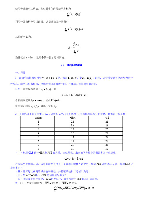
2.8 3.4 3.0 3.5 3.6 3.0 2.7 3.7
21 24 26 27 29 25 25 30
(Ⅰ)利用 OLS 估计 GPA 和 ACT 的关系;也就是说,求出如下方程中的截距和斜率估计值
ˆ ˆ ACT GPA 0 1
评价这个关系的方向。这里的截距有没有一个有用的解释?请说明。如果 ACT 分数提高 5 分,预期 GPA 会 提高多少? (Ⅱ)计算每次观测的拟合值和残差,并验证残差和(近似)为零。 (Ⅲ)当 ACT 20 时, GPA 的预测值为多少? (Ⅳ)对这 8 个学生来说, GPA 的变异中,有多少能由 ACT 解释?试说明。 答: (Ⅰ)变量的均值为: GPA 3.2125 , ACT 25.875 。
- 1、下载文档前请自行甄别文档内容的完整性,平台不提供额外的编辑、内容补充、找答案等附加服务。
- 2、"仅部分预览"的文档,不可在线预览部分如存在完整性等问题,可反馈申请退款(可完整预览的文档不适用该条件!)。
- 3、如文档侵犯您的权益,请联系客服反馈,我们会尽快为您处理(人工客服工作时间:9:00-18:30)。
DATA SET HANDBOOKIntroductory Econometrics: A Modern Approach, 4eJeffrey M. WooldridgeThis document contains a listing of all data sets that are provided with the fourth edition of Introductory Econometrics: A Modern Approach. For each data set, I list its source (wherever possible), where it is used or mentioned in the text (if it is), and, in some cases, notes on how an instructor might use the data set to generate new homework exercises, exam problems, or term projects. In some cases, I suggest ways to improve the data sets.Special thanks to Edmund Wooldridge, who provided valuable assistance in updating the page numbers for the fourth edition.401K.RAWSource:L.E. Papke (1995), “Participation in and Contributions to 401(k) Pension Plans: Evidence from Plan Data,”Journal of Human Resources 30, 311-325.Professor Papke kindly provided these data. She gathered them from the Internal Revenue Service’s Form 5500 tapes.Used in Text: pages 64, 80, 135-136, 173, 217, 685-686Notes: This data set is used in a variety of ways in the text. One additional possibility is to investigate whether the coefficients from the regression of prate on mrate, log(totemp) differ by whether the plan is a sole plan. The Chow test (see Section 7.4), and the less restrictive version that allows different intercepts, can be used.401KSUBS.RAWSource: A. Abadie (2003), “Semiparametric Instrumental Variable Estimation of Treatment Response Models,”Journal of Econometrics 113, 231-263.Professor Abadie kindly provided these data. He obtained them from the 1991 Survey of Income and Program Participation (SIPP).Used in Text: pages 165, 182, 222, 261, 279-280, 288, 298-299, 336, 542Notes: This data set can also be used to illustrate the binary response models, probit and logit, in Chapter 17, where, say, pira (an indicator for having an individual retirement account) is the dependent variable, and e401k [the 401(k) eligibility indicator] is the key explanatory variable.ADMNREV.RAWSource:Data from the National Highway Traffic Safety Administration: “A Digest of State Alcohol-Highway Safety Related Legislation,” U.S. Department of Transportation, NHTSA. I used the third (1985), eighth (1990), and 13th (1995) editions.Used in Text: not usedNotes: This is not so much a data set as a summary of so-called “administrative per se” laws at the state level, for three different years. It could be supplemented with drunk-driving fatalities for a nice econometric analysis. In addition, the data for 2000 or later years can be added, forming the basis for a term project. Many other explanatory variables could be included. Unemployment rates, state-level tax rates on alcohol, and membership in MADD are just a few possibilities.AFFAIRS.RAWSource: R.C. Fair (1978), “A Theory of Extramarital Affairs,”Journal of Political Economy 86, 45-61, 1978.I collected the data from P rofessor Fair’s web cite at the Yale University Department of Economics. He originally obtained the data from a survey by Psychology Today.Used in Text: not usedNotes: This is an interesting data set for problem sets, starting in Chapter 7. Even though naffairs (number of extramarital affairs a woman reports) is a count variable, a linear model can be used as decent approximation. Or, you could ask the students to estimate a linear probability model for the binary indicator affair, equal to one of the woman reports having any extramarital affairs. One possibility is to test whether putting the single marriage rating variable, ratemarr,is enough, against the alternative that a full set of dummy variables is needed; see pages 237-238 for a similar example. This is also a good data set to illustrate Poisson regression (using naffairs) in Section 17.3 or probit and logit (using affair) in Section 17.1.AIRFARE.RAWSource: Jiyoung Kwon, a doctoral candidate in economics at MSU, kindly provided these data, which she obtained from the Domestic Airline Fares Consumer Report by the U.S. Departmentof Transportation.Used in Text: pages 501-502, 573Notes: This data set nicely illustrates the different estimates obtained when applying pooled OLS, random effects, and fixed effects.APPLE.RAWSource: These data were used in the doctoral dissertation of Jeffrey Blend, Department of Agricultural Economics, Michigan State University, 1998. The thesis was supervised by Professor Eileen van Ravensway. Drs. Blend and van Ravensway kindly provided the data, which were obtained from a telephone survey conducted by the Institute for Public Policy and Social Research at MSU.Used in Text: pages 199, 222, 263, 618Notes: This data set is close to a true experimental data set because the price pairs facing a family were randomly determined. In other words, the family head was presented with prices for the eco-labeled and regular apples, and then asked how much of each kind of apple they would buy at the given prices. As predicted by basic economics, the own price effect is strongly negative and the cross price effect is strongly positive. While the main dependent variable, ecolbs, piles up at zero, estimating a linear model is still worthwhile. Interestingly, because the survey design induces a strong positive correlation between the prices of eco-labeled and regular apples, there is an omitted variable problem if either of the price variables is dropped from the demand equation. A good exam question is to show a simple regression of ecolbs on ecoprc and then a multiple regression on both prices, and ask students to decide whether the price variables must be positively or negatively correlated.ATHLET1.RAWSources: Peterson's Guide to Four Year Colleges, 1994 and 1995 (24th and 25th editions). Princeton University Press. Princeton, NJ.The Official 1995 College Basketball Records Book, 1994, NCAA.1995 Information Please Sports Almanac (6th edition). Houghton Mifflin. New York, NY. Used in Text: page 690Notes: These data were collected by Patrick Tulloch, an MSU economics major, for a term project. The “athletic success” var iables are for the year prior to the enrollment and academic data. Updating these data to get a longer stretch of years, and including appearances in the “Sweet 16” NCAA basketball tournaments, would make for a more convincing analysis. With the growing popularity of women’s sports, especially basketball, an analysis that includes success in w omen’s athletics would be interesting.ATHLET2.RAWSources: Peterson's Guide to Four Year Colleges, 1995 (25th edition). Princeton University Press.1995 Information Please Sports Almanac (6th edition). Houghton Mifflin. New York, NY Used in Text: page 690Notes: These data were collected by Paul Anderson, an MSU economics major, for a term project. The score from football outcomes for natural rivals (Michigan-Michigan State, California-Stanford, Florida-Florida State, to name a few) is matched with application and academic data. The application and tuition data are for Fall 1994. Football records and scores are from 1993 football season. Extended these data to obtain a long stretch of panel data and other “natural” rivals could be very interesting.ATTEND.RAWSource: These data were collected by Professors Ronald Fisher and Carl Liedholm during a term in which they both taught principles of microeconomics at Michigan State University. Professors Fisher and Liedholm kindly gave me permission to use a random subset of their data, and their research assistant at the time, Jeffrey Guilfoyle, who completed his Ph.D. in economics at MSU, provided helpful hints.Used in Text: pages 111, 151, 198-199, 220-221Notes: The attendance figures were obtained by requiring students to slide their ID cards through a magnetic card reader, under the supervision of a teaching assistant. You might have the students use final, rather than the standardized variable, so that they can see the statistical significance of each variable remains exactly the same. The standardized variable is used only so that the coefficients measure effects in terms of standard deviations from the average score.AUDIT.RAWSource: These data come from a 1988 Urban Institute audit study in the Washington, D.C. area.I obtained them from the article “The Urban Institute Audit Studies: Their Methods and Findings,” by James J. Heckman and Peter Siegelman. In Fix, M. and Struyk, R., eds., Clear and Convincing Evidence: Measurement of Discrimination in America. Washington, D.C.: Urban Institute Press, 1993, 187-258.Used in Text: pages 768-769, 776, 779BARIUM.RAWSource: C.M. Krupp and P.S. Pollard (1999), "Market Responses to Antidumpting Laws: Some Evidence from the U.S. Chemical Industry," Canadian Journal of Economics 29, 199-227. Dr. Krupp kindly provided the data. They are monthly data covering February 1978 through December 1988.Used in Text: pages 357-358, 369, 373, 418, 422-423, 440, 655, 657, 665Note: Rather than just having intercept shifts for the different regimes, one could conduct a full Chow test across the different regimes.BEAUTY.RAWSource: Hamermesh, D.S. and J.E. Biddle (1994), “Beauty and the Labor Market,” American Economic Review 84, 1174-1194.Professor Hamermesh kindly provided me with the data. For manageability, I have included only a subset of the variables, which results in somewhat larger sample sizes than reported for the regressions in the Hamermesh and Biddle paper.Used in Text: pages 236-237, 262-263BWGHT.RAWSource: J. Mullahy (1997), “Instrumental-Variable Estimation of Count Data Models: Applications to Models of Cigarette Smoking Beh avior,” Review of Economics and Statistics 79, 596-593.Professor Mullahy kindly provided the data. He obtained them from the 1988 National Health Interview Survey.Used in Text: pages 18, 62, 110, 150-151, 164, 176, 182, 184-187, 255-256, 515-516 BWGHT2.RAWSource: Dr. Zhehui Luo, a recent MSU Ph.D. in economics and Visiting Research Associate in the Department of Epidemiology at MSU, kindly provided these data. She obtained them from state files linking birth and infant death certificates, and from the National Center for Health Statistics natality and mortality data.Used in Text: pages 165, 211-222Notes: There are many possibilities with this data set. In addition to number of prenatal visits, smoking and alcohol consumption (during pregnancy) are included as explanatory variables. These can be added to equations of the kind found in Exercise C6.10. In addition, the one- and five-minute APGAR scores are included. These are measures of the well being of infants just after birth. An interesting feature of the score is that it is bounded between zero and 10, making a linear model less than ideal. Still, a linear model would be informative, and you might ask students about predicted values less than zero or greater than 10.CAMPUS.RAWSource: These data were collected by Daniel Martin, a former MSU undergraduate, for a final project. They come from the FBI Uniform Crime Reports and are for the year 1992.Used in Text: pages 130-131Notes: Colleges and universities are now required to provide much better, more detailed crime data. A very rich data set can now be obtained, even a panel data set for colleges across different years. Statistics on male/female ratios, fraction of men/women in fraternities or sororities, policy variables – s uch as a “safe house” for women on campus, as was started at MSU in 1994 – could be added as explanatory variables. The crime rate in the host town would be a good control. CARD.RAWSource: D. Card (1995), "Using Geographic Variation in College Proximity to Estimate the Return to Schooling," in Aspects of Labour Market Behavior: Essays in Honour of John Vanderkamp. Ed. L.N. Christophides, E.K. Grant, and R. Swidinsky, 201-222. Toronto: University of Toronto Press.Professor Card kindly provided these data.Used in Text: pages 519-520, 540Notes: Computer Exercise C15.3 is important for analyzing these data. There, it is shown that the instrumental variable, nearc4, is actually correlated with IQ, at least for the subset of men for which an IQ score is reported. However, the correlation between nearc4 and IQ, once the other explanatory variables are netted out, is arguably zero. (At least, it is not statistically different from zero.) In other words, nearc4 fails the exogeneity requirement in a simple regression model but it passes – at least using the crude test described above – if controls are added to the wage equation.For a more advanced course, a nice extension of Card’s analysis is to allow the return to education to differ by race. A relatively simple extension is to include black⋅educ as an additional explanatory variable; its natural instrument is black⋅nearc4.CEMENT.RAW:Source: J. Shea (1993), “The Input-Output Approach to Instrument Selection,”Journal of Business and Economic Statistics 11, 145-156.Professor Shea kindly provided these data.Used in Text: pages 571-572Notes: Compared with Shea’s analysis, the producer price index (PPI) for fuels and power has been replaced with the PPI for petroleum. The data are monthly and have not been seasonally adjusted.CEOSAL1.RAWSource: I took a random sample of data reported in the May 6, 1991 issue of Businessweek.Used in Text: pages 33-34, 36-37, 40, 159, 216, 256-257, 260, 685, 691Notes: This kind of data collection is relatively easy for students just learning data analysis, and the findings can be interesting. A good term project is to have students collect a similar data set using a more recent issue of Businessweek, and to find additional variables that might explain differences in CEO compensation. My impression is that the public is still interested in CEO compensation.An interesting question is whether the list of explanatory variables included in this data set now explain less of the variation in log(salary) than they used to.CEOSAL2.RAWSource: See CEOSAL1.RAWUsed in Text: pages 65, 111, 163, 212-213, 332, 691Notes: Compared with CEOSAL1.RAW, in this CEO data set more information about the CEO, rather than about the company, is included.CHARITY.RAWSource: P.H. Franses and R. Paap (2001), Quantitative Models in Marketing Research. Cambridge: Cambridge University Press.Professor Franses kindly provided the data.Used in Text: pages 66, 112-113, 263, 619-620Notes: This data set can be used to illustrate probit and Tobit models, and to study the linear approximations to them.CONSUMP.RAWSource: I collected these data from the 1997 Economic Report of the President. Specifically, the data come from Tables B-71, B-15, B-29, and B-32.Used in Text: pages 374, 406, 439, 563, 571, 665-666 Notes: For a student interested in time series methods, updating this data set and using it in a manner similar to that in the text could be acceptable as a final project.CORN.RAWSource: G.E. Battese, R.M. Harter, and W.A. Fuller (1988), “An Error-Components Model for Prediction of County Crop Areas Using Survey and Satellite Data,” Journal of the American Statistical Association 83, 28-36.This small data set is reported in the article.Used in Text: pages 783-784Notes: You could use these data to illustrate simple regression when the population intercept should be zero: no corn pixels should predict no corn planted. The same can be done with the soybean measures in the data set.CPS78_85.RAWSource: Professor Henry Farber, now at Princeton University, compiled these data from the 1978 and 1985 Current Population Surveys. Professor Farber kindly provided these data when we were colleagues at MIT.Used in Text: pages 447-448, 473-474Notes: Obtaining more recent data from the CPS allows one to track, over a long period of time, the changes in the return to education, the gender gap, black-white wage differentials, and the union wage premium.CPS91.RAWSource: Professor Daniel Hamermesh, at the University of Texas, compiled these data from the May 1991 Current Population Survey. Professor Hamermesh kindly provided these data.Used in Text: page 619Notes: This is much bigger than the other CPS data sets, and it is much bigger thanMROZ.RAW, too. In addition to the usual productivity factors for the women in the sample, we have information on the husband. Therefore, we can estimate a labor supply function as in Chapter 16, although the validity of potential experience as an IV for log(wage) is questionable. (MROZ.RAW contains an actual experience variable.) Perhaps more convincing is to add hours to the wage offer equation, and instrument hours with indicators for young and old children. This data set also contains a union indicator.The web site for the National Bureau of Economic Research makes it very easy now to download data CPS data files in a variety of formats. Go to /data/cps_basic.html. CRIME1.RAWSource: J. Grogger (1991), “Certainty vs. Severity of Punishment,” Economic Inquiry 29, 297-309.Professor Grogger kindly provided a subset of the data he used in his article.Used in Text: pages 82-83, 172-173, 178, 250-251, 270-271, 296, 301-303, 598-600, 616CRIME2.RAWSource: These data were collected by David Dicicco, a former MSU undergraduate, for a final project. They came from various issues of the County and City Data Book, and are for the years 1982 and 1985. Unfortunately, I do not have the list of cities.Used in Text: pages 311-312, 455-459Notes: Very rich crime data sets, at the county, or even city, level, can be collected using the FBI’s Uniform Crime Reports. These data can be matched up with demographic and economic data, at least for census years. The County and City Data Book contains a variety of statistics,but the years do not always match up. These data sets can be used investigate issues such as the effects of casinos on city or county crime rates.CRIME3.RAW:Source: E. Eide (1994), Economics of Crime: Deterrence of the Rational Offender. Amsterdam: North Holland. The data come from Tables A3 and A6.Used in Text: pages 461, 475Notes: These data are for the years 1972 and 1978 for 53 police districts in Norway. Much larger data sets for more years can be obtained for the United States, although a measure of the “clear-up” rate is needed.CRIME4.RAWSource: From C. Cornwell an d W. Trumball (1994), “Estimating the Economic Model of Crime with Panel Data,” Review of Economics and Statistics 76, 360-366.Professor Cornwell kindly provided the data.Used in Text: pages 468-469, 476, 498-499, 572Notes: Computer Exercise C16.7 shows that variables that might seem to be good instrumental variable candidates are not always so good, especially after applying a transformation such as differencing across time. You could have the students do an IV analysis for just, say, 1987.DISCRIM.RAWSource: K. Graddy (1997), "Do Fast-Food Chains Price Discriminate on the Race and Income Characteristics of an Area?" Journal of Business and Economic Statistics 15, 391-401. Professor Graddy kindly provided the data set.Used in Text: pages 112, 165, 692Notes: If you want to assign a common final project, this would be a good data set. There are many possible dependent variables, namely, prices of various fast-food items. The key variable is the fraction of the population that is black, along with controls for poverty, income, housing values, and so on. These data were also used in a famous study by David Card and Alan Krueger on estimation of minimum wage effects on employment. See the book by Card and Krueger, Myth and Measurement, 1997, Princeton University Press, for a detailed analysis.EARNS.RAWSource: Economic Report of the President, 1989, Table B 47. The data are for the non-farm business sector.Used in Text: pages 360, 395-396, 404Notes: These data could be usefully updated, but changes in reporting conventions in more recent ERP s may make that difficult.ELEM94_95.RAWSource: Culled from a panel data set used by Leslie Papke in her paper “The Effects of Spending on Test Pass Rates: Evidence from Michigan” (2005), Journal of Public Economics 89, 821-839. Used in Text: pages 166, 337Notes: Starting in 1995, the Michigan Department of Education stopped reporting average teacher benefits along with average salary. This data set includes both variables, at the school level, and can be used to study the salary-benefits tradeoff, as in Chapter 4. There are a few suspicious benefits/salary ratios, and so this data set makes a good illustration of the impact of outliers in Chapter 9.ENGIN.RAWSource: Thada Chaisawangwong, a graduate student at MSU, obtained these data for a term project in applied econometrics. They come from the Material Requirement Planning Survey carried out in Thailand during 1998.Used in Text: not usedNotes: This is a nice change of pace from wage data sets for the United States. These data are for engineers in Thailand, and represents a more homogeneous group than data sets that consist of people across a variety of occupations. Plus, the starting salary is also provided in the data set, so factors affecting wage growth – and not just wage levels at a given point in time – can be studied. This is a good data set for a common term project that tests basic understanding of multiple regression and the interpretation of models with a logarithm for a dependent variable. EZANDERS.RAWSource: L.E. Papke (1994), “Tax Policy and Urban Development: Evidence from the Indiana Enterprise Zone Program,” Journal of Public Economics 54, 37-49.Professor Papke kindly provided these data.Used in Text: page 374Notes: These are actually monthly unemployment claims for the Anderson enterprise zone. Papke used annualized data, across many zones and non-zones, in her analysis.EZUNEM.RAWSource: See EZANDERS.RAWUsed in Text: pages 467-468, 499Notes: A very good project is to have students analyze enterprise, empowerment, or renaissance zone policies in their home states. Many states now have such programs. A few years of panel data straddling periods of zone designation, at the city or zip code level, could make a nice study.FAIR.RAWSource: R.C. Fair (1996), “Econometrics and Presidential Elections,” Journal of Economic Perspectives 10, 89-102.The data set is provided in the article.Used in Text: pages 358-360, 438, 439Notes: An updated version of this data set, through the 2004 election, is available at Professor Fair’s web site at Yale University: /rayfair/pdf/2001b.htm. Students might want to try their own hands at predicting the most recent election outcome, but they should be restricted to no more than a handful of explanatory variables because of the small sample size.FERTIL1.RAWSource: W. Sander, “The Effect of Women’s Schooling on Fertility,” Economics Letters 40, 229-233.Professor Sander kindly provided the data, which are a subset of what he used in his article. He compiled the data from various years of the National Opinion Resource Center’s General Social Survey.Used in Text: pages 445-447, 473, 534, 617, 673Notes: (1) Much more recent data can be obtained from the National Opinion Research Center website, /GSS+Website/Download/. Very rich pooled cross sections can be constructed to study a variety of issues – not just changes in fertility over time.It would be interesting to analyze a similar data set for a developing country, especially where efforts have been made to emphasize birth control. Some measure of access to birth control could be useful if it varied by region. Sometimes, one can find policy changes in the advertisement or availability of contraceptives.FERTIL2.RAWSource: These data were obtained by James Heakins, a former MSU undergraduate, for a term project. They come from Botswana’s 1988 Demographic and Health Survey.Used in Text: page 540Notes: Currently, this data set is used only in one computer exercise. Since the dependent variable of interest – number of living children or number of children every born – is a count variable, the Poisson regression model discussed in Chapter 17 can be used. However, some care is required to combine Poisson regression with an endogenous explanatory variable (educ).I refer you to Chapter 19 of my book Econometric Analysis of Cross Section and Panel Data. Even in the context of linear models, much can be done beyond Computer Exercise C15.2. At a minimum, the binary indicators for various religions can be added as controls. One might also interact the schooling variable, educ, with some of the exogenous explanatory variables.FERTIL3.RAWSource: L.A. Whittington, J. Alm, and H.E. Peters (1990), “Fertility and the Personal Exemption: Implicit Pronatalist Pol icy in the United States,” American Economic Review 80, 545-556.The data are given in the article.Used in Text: pages 354-355, 364, 373, 374, 394-395, 398, 405, 438, 641, 658-659, 664, 665FISH.RAWSource: K Graddy (1995), “Testing for Imperfect Competition at the Fulton Fish Market,” RAND Journal of Economics 26, 75-92.Professor Graddy's collaborator on a later paper, Professor Joshua Angrist at MIT, kindly provided me with these data.Used in Text: pages 440, 572Notes: This is a nice example of how to go about finding exogenous variables to use as instrumental variables. Often, weather conditions can be assumed to affect supply while having a negligible effect on demand. If so, the weather variables are valid instrumental variables for price in the demand equation. It is a simple matter to test whether prices vary with weather conditions by estimating the reduced form for price.FRINGE.RAWSource: F. Vella (1993), “A Simple Estimator for Simultaneous Models with Censored Endogenous Regre ssors,” International Economic Review 34, 441-457.Professor Vella kindly provided the data.Used in Text: page 616Notes: Currently, this data set is used in only one Computer Exercise – to illustrate the Tobit model. It can be used much earlier. First, one could just ignore the pileup at zero and use a linear model where any of the hourly benefit measures is the dependent variable. Another possibility is to use this data set for a problem set in Chapter 4, after students have read Example 4.10. That example, which uses teacher salary/benefit data at the school level, finds the expected tradeoff, although it appears to less than one-to-one. By contrast, if you do a similar analysis with FRINGE.RAW, you will not find a tradeoff. A positive coefficient on the benefit/salary ratio is not too surprising because we probably cannot control for enough factors, especially when looking across different occupations. The Michigan school-level data is more aggregated than one would like, but it does restrict attention to a more homogeneous group: high school teachers in Michigan.GPA1.RAWSource: Christopher Lemmon, a former MSU undergraduate, collected these data from a survey he took of MSU students in Fall 1994.Used in Text: pages 75-76, 78, 81-82, 128-130, 160, 230, 258-259, 292-293, 297-298, 813-814 Notes: This is a nice example of how students can obtain an original data set by focusing locally and carefully composing a survey.GPA2.RAWSource: For confidentiality reasons, I cannot provide the source of these data. I can say that they come from a midsize research university that also supports men’s and women’s athletics at the Division I level.Used in Text: pages 105-106, 182, 207, 209, 219, 256, 259-260GPA3.RAWSource: See GPA2.RAWUsed in Text: pages 244-246, 269, 294-295, 475HPRICE1.RAW。