
接触分析实例
Library of Element Types (单元类型库)对话框。 2.在单元类型库对话框中,靠近左边的列表中,单击“Structural Solid”一次, 使其高亮度显示,指定添加的单元类型为结构实体单元。然后,在靠近右边的列 表中,单击“Brick 8node 185”一次,选定单元类型Solid185 为第一类单元。单击 对话框中的OK按钮,关闭Library of Element Types 对话框。然后,Element Types (单元类型)对话框会重新显示,且在对话框中的单元列表框中列出了定义 的单元类型1:Solid185。 3.单击Element Types (单元类型定义)对话框中的Close按钮,关闭对话框,完成 单元类型的定义。
完成对标题名的指定。
应用力学研究所
李永强
§16.2 建立有限元模型
设置分析标题
3.选取菜单路径Utility Menu | Plot | Replot,指定的标题“Analysis of a
Axis Contacting a hole in a Disc”将显示在图形窗口的左下角。
4.选取菜单路径Main Menu | Preference,将弹出Preference of GUI Filtering (菜单过滤参数选择)对话框。单击Structual(结构)选项使之被选
中,以将菜单设置为与结构分析相关的选项。单击OK按钮关闭,完成分
析范畴的指定。
应用力学研究所
李永强
§16.2 建立有限元模型
定义单元类型
本实例分析的问题中涉及到大变形,故选用Solid185单元类型来建立本实例 的模型。本接触问题属于面面接触,目标面和接触面都是柔性的,将使用接触单 元TARGE170和CONTA174来模拟接触面。接触单元在分析过程中使用接触向导 时可以自动添加,这里就不再添加。下面为定义单元类型的具体操作过程。 1.选取菜单路径Main Menu | Preprocessor | Element Type | Add/Edit/Delete,将 弹出Element Types (单元类型)对话框。单击对话框中的Add按钮,将弹出
应用力学研究所
李永强
§16.2 建立有限元模型
在ANSYS中,首先我们通过完成如下工作来建立本实例的有限 元模型,需要完成的工作有:指定分析标题,定义单元类型,定义 材料性能,建立结构几何模型、进行网格划分等。根据本实例的结 构特点,我们将首先建立代表盘和轴的两个1/4圆环面,然后对其进 行网格划分,得到有限元模型。
应用力学研究所
李永强§16.1 问题描述源自由于模型和载荷都是轴对称的,可以用轴对称方法进行分析。这
里为了后处理时观察结果更直观,我们采用整个模型的四分之一进行
建模分析,最后将其进行扩展,来观察整个结构的变形及应力分布、 变化情况。盘和轴用同一种材料,其性质如下: 弹性模量: EX=2.1E5 泊松比: NUXY=0.3 接触摩擦系数 : MU=0.2
应用力学研究所
李永强
§16.2 建立有限元模型
定义材料特性
本实例中盘轴使用同一种材料类型,所以只需定义一种材料就可以了。下
面是具体的操作过程。
1.选取菜单路径Main Menu | Preprocessor | Material Props | Material Models, 将弹出Define Material Model Behavior (材料模型定义)对话框。 2.在对话框的右边选项框中,依次双击Structural | Linear | Elastic | Isotropic, 将弹出1号材料的弹性模量EX和泊松比PRXY的定义对话框。 3.在线性各向同性材料属性对话框中的EX (弹性模量)文本框中输入“2.1E5”, PRXY (泊松比)文本框中输入0.3。单击对话框中的OK按钮关闭对话框。
工程结构分析软件
第16章 接触分析实例
应用力学研究所
李永强
第16章 接触分析实例
在这个实例中,将对一个盘轴紧 配合结构进行接触分析。第一个载荷 步分析轴和盘在过盈配合时的应力, 第二个载荷步分析将该轴从盘心拔出 时轴和盘的接触应力情况。
应用力学研究所
李永强
第16章 接触分析实例
§16.1 问题描述 §16.2 建立有限元模型
设置分析标题 定义单元类型 定义材料特性 建立几何模型并分网 创建接触对
应用力学研究所 李永强
§16.2 建立有限元模型
设置分析标题
本实例为进行盘轴结构的接触分析,属于非线性结构分析范畴。跟前面
实例一样,为了在后面进行菜单方式操作时的方便,需要在开始分析时就指
定本实例分析范畴为“Structural”。本实例的标题可以命名为:“Analysis of a Axis Contacting a hole in a Disc”,具体的操作过程如下: 1.选取菜单路径Utility Menu | File | Change Jobname,将弹出Change Jobname (修改文件名)对话框。在Enter new jobname (输入新文件名)文本框 中输入文字“CH16”,为本分析实例的数据库文件名。并单击New log and error files (新的日志和错误文件)单选框,使其变为“Yes”,为本实例的分析 过程创建新的日志。单击OK按钮关闭对话框,完成文件名的修改。 2.选取菜单路径Utility Menu | File | Change Title,将弹出Change Title (修 改标题)对话框。在Enter new title (输入新标题)文本框中输入文字“Analysis of a Axis Contacting a hole in a Disc”,为本分析实例的标题名。单击OK按钮,
§16.3 加载并求解
§16.4 结果分析 §16.5 命令流输入
应用力学研究所 李永强
§16.1 问题描述
在旋转机械中通常会遇到轴与轴承、轴与齿轮、轴与盘连接的问题, 根据各自的不同情况可能有不同的连接形式。但大多数连接形式中存在过 盈配合,也就是涉及到接触问题的分析。这里我们以某转子中轴和盘的连 接为例,分析轴和盘的配合应力以及将轴从盘中拔处时盘轴连接处的应力 情况。 本实例的轴为一等直径空心轴,盘为等厚度圆盘,其结构及尺寸 如图所示。
ABAQUS应用培训-09 接触分析及实例
15
2015/7/5
15
4
2015/7/5
4
接触 –利用接触模块定义并管理以下信息:
– 模型区域之间或模型区域同它周围模型之间的机械和热接触。
机械接触 一般和双面接触 自接触 弹性基础 激励器/传感器
其它接触 (约束) 捆绑约束 刚体 显示体 耦合 壳到实体耦合 嵌入区域 线性多点约束方程
热接触 热膜条件 对环境的辐射 热接触
1
4
5
2 7
3 10
6 11
8
9
12
3
接触操作(Interaction)
Interaction
1. 不同的接触算法:standard explicit 2. 作为一种边界条件,接触定义在不同的step中可以发生变化 3. 接触算法还分为Kinematic, Penalty,初学者不用选择 4. Surface to Surface, Surface to node 5. 主面(master, first)和从面(slace,second) 6. 接触体之间的相互作用:摩擦和热传递等设置 7. 接触面的间隙调整
k14 k24 k34 k44 k54 k64 0 0 0 0 0 0
0 0 k35 k45 k55 k65 0 0 0 0 0 0
0 0 k36 k 46 k56 k66 0 0 0 0
k116 0
0 0 0 0 0 0 k77 k87 k97 k107 0 0
0 0 0 0 0 0 k78 k88 k98 k108 0 0
有限元分析-ABAQUS的应用
接触分析
方 刚
2015年7月
2015/7/5
1
1
接触
• “为什么要定义机械接触?
酒精过敏实例分析报告

酒精过敏实例分析报告酒精过敏是一种较为常见的过敏症状,患者在接触酒精后会出现过敏反应,包括皮肤发红、瘙痒、呼吸困难、恶心、呕吐等症状。
本文将就一位患者的酒精过敏实例进行分析,并给出相应的治疗建议。
患者,女性,30岁,平时偶尔会饮酒。
最近一次聚会时,患者饮用了一杯啤酒后,不久就出现皮肤发红、瘙痒的症状。
她没有任何过敏史,并且之前也饮过酒,没有出现过类似的反应。
由于症状较为明显,患者随即就就诊于附近的医院。
根据患者的症状和个人史,医生初步判断为酒精过敏。
在问诊过程中,医生发现患者在近期没有接触过其他可能导致过敏的物质,不存在其他过敏的可能性。
基于这些信息,医生向患者解释了酒精过敏的原理。
酒精过敏是一种免疫系统不良反应,通常是由于酒精中的某些成分引起的。
对于大多数人来说,人体可以正常代谢酒精,并将其分解为二氧化碳和水。
然而,对于一些人来说,他们的免疫系统会对酒精中的成分产生不良反应,导致过敏症状的发生。
酒精过敏的原因是多种多样的,可能是由于酒精中的添加剂、防腐剂或其他化学物质引起的。
对于患者来说,可能是啤酒中某种特定的成分引发了过敏反应。
医生建议患者进行酒精过敏的相关测试,以确定过敏原的具体成分。
针对患者的症状,医生给予了以下的治疗建议和措施:1. 避免饮用含酒精的饮品:为了避免再次发生过敏反应,患者需要避免饮用一切含酒精的饮品,包括啤酒、葡萄酒、烈酒等。
2. 使用抗过敏药物:患者可以在医生的指导下使用抗过敏药物,如抗组胺药物,来缓解症状和减轻过敏反应的程度。
3. 饮食调整:患者需要注意饮食,避免食用含酒精成分较高的食物,如糕点、酱料等,以免再次引发过敏反应。
4. 寻求专业意见:患者可以寻求专业的过敏专科医生的意见,进一步进行过敏相关测试,以确定过敏原的具体成分,从而采取更有针对性的治疗措施。
综上所述,酒精过敏是一种相对常见的过敏症状,但具体原因可能因人而异。
对于患者而言,了解过敏发生的原理和可能的过敏原是非常有帮助的。
ansysworkbench 接触实例分析
前言WokBench 是众所周知的好东西,以下是自己琢磨的一个小应用,肯定有不对的地方,欢迎指出,便于大家共同提高。
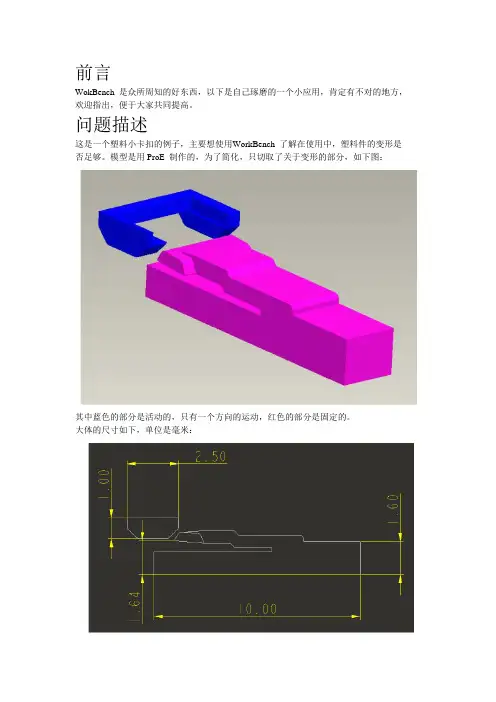
问题描述这是一个塑料小卡扣的例子,主要想使用WorkBench 了解在使用中,塑料件的变形是否足够。
模型是用ProE 制作的,为了简化,只切取了关于变形的部分,如下图:其中蓝色的部分是活动的,只有一个方向的运动,红色的部分是固定的。
大体的尺寸如下,单位是毫米:注意:在模型中,蓝色和红色部件的距离要控制好(这是由ProE 中,模型装配关系决定的),如果太近,软件将自动计算出一个接触区域,但对于这个例子,还需要手动扩大接触区域。
如果距离太远,在手动设置Pinball 类型的接触区域时,Pinball 的半径要设得很大,可能导致无法计算。
请参考上面的尺寸图纸调节两个部件之间的距离。
之后,设置接触面(2、3):需要将两个部件在运动过程中,会接触的地方一一标出,千万不要加无用的面。
将Pinball Region 设置为Radius 方式(4),并将Radius 设置一个合适的值(5),本例设置了3 毫米(如图,会形成一个蓝色的大圆球),求解的时候软件会使用这个PinBall 自动探测接触。
还需要将接触方式设置为无摩擦的(6)。
最后将接触面计算方式设置为Adjust To Touch(7)。
也可以尝试其他的方式,不过对于这个仅研究红色部件变形的例子就无所谓了。
关于单元格WorkBench 中可以不自行划分单元格(在解算的时候,如果没有手动的设置,软件就会先自动划分),软件帮你自动产生。
如果你的其他设置正确,即便是这个自动的值也能很精确了。
添加分析这个分析用静力学就可以了(1)。
之后要设置Analysis Setting(2)。
将Nuber Of Step 设置为2(3)。
注意:1)蓝色部件在运动的过程中,先压迫红色部件,再逐渐松开,因此必须将这个过程至少分解为至少两个阶段(阶段指“Step”)。
ANSYS接触实例分析参考

ANSYS接触实例分析参考1.实例描述一个钢销插在一个钢块中的光滑销孔中。
已知钢销的半径是0.5 units, 长是2.5 units,而钢块的宽是 4 Units, 长4 Units,高为1 Units,方块中的销孔半径为0.49 units,是一个通孔。
钢块与钢销的弹性模量均为36e6,泊松比为0.3.由于钢销的直径比销孔的直径要大,所以它们之间是过盈配合。
现在要对该问题进行两个载荷步的仿真。
(1)要得到过盈配合的应力。
(2)要求当把钢销从方块中拔出时,应力,接触压力及约束力。
2.问题分析由于该问题关于两个坐标面对称,因此只需要取出四分之一进行分析即可。
进行该分析,需要两个载荷步:第一个载荷步,过盈配合。
求解没有附加位移约束的问题,钢销由于它的几何尺寸被销孔所约束,由于有过盈配合,因而产生了应力。
第二个载荷步,拔出分析。
往外拉动钢销1.7 units,对于耦合节点上使用位移条件。
打开自动时间步长以保证求解收敛。
在后处理中每10个载荷子步读一个结果。
本篇先谈第一个载荷步的计算。
下篇再谈第二个载荷步的计算。
3.读入几何体首先打开ANSYS APDL然后读入已经做好的几何体。
从【工具菜单】-->【File】-->【Read Input From】打开导入文件对话框找到ANSYS自带的文件(每个ansys都自带的)\Program Files\Ansys Inc\V145\ANSYS\data\models\block.inp【OK】后,四分之一几何模型被导入。
4.定义单元类型只定义实体单元的类型SOLID185。
至于接触单元,将在下面使用接触向导来定义。
5.定义材料属性只有线弹性材料属性:弹性模量36E6和泊松比0.36.划分网格打开MESH TOOL,先设定关键地方的网格划分份数然后在MESH TOOL中设定对两个体均进行扫略划分,在volumeSweeping中选择pick all,按下【Sweep】按钮,在主窗口中选择两个体,进行网格划分。
本文介绍了ANSYS APDL命令和轴承接触分析相关实例

本文介绍了ANSYS APDL命令和轴承接触分析相关实例。
finish/clear/filename,ex5-3 !设定工作名/title,the contact analysis of Bearing !设定工作标题!************************************!进入前处理模块!************************************/prep7*set,roll_r,5.7 !定义变量参数*set,inside_r1,15*set,inside_r2,18.5*set,outside_r1,29.8*set,outside_r2,33.3*set,deep,8*set,axes_r3,15.5*set,fillet_r4,1*set,axes_deep,20*set,fillet_r5,1!定义单元类型和属性et,1,solid45 !定义单元类型solid45MP,EX,1,2.06e5 !定义弹性模量MP,PRXY,1,0.3 !定义泊松比MP,MU,1,0.3 !定义摩擦系数!建立模型sph4,,-inside_r2-roll_r,roll_r+0.9 !生成轴承滚珠cyl4,,,inside_r1,-120,inside_r2,-60,deep !生成+z向的轴承内圈cyl4,,,outside_r1,-120,outside_r2,-60,deep !生成+z向的轴承外圈cyl4,,,inside_r1,-120,inside_r2,-60,-deep !生成-z向的轴承内圈cyl4,,,outside_r1,-120,outside_r2,-60,-deep !生成-z向的轴承外圈wpoff,0,0,-deep !偏移工作平面cyl4,,,0,-120,axes_r3,-60,-axes_deep !生成装配轴lfillt,57,59,fillet_r4,, !生成倒角线al,57,62,59,54,61 !由线生成面vrotat,32,,,,,,42,37,60,1, !旋转面生成体vdele,6,,,1 !删除编号为6的体!lfillt,31,39,fillet_r5,, !生成倒角线al,34,39,53,31,37 !由线生成面vdrag,27,,,,,,35 !拖拉面生成体vdele,4,,,1 !删除编号为4的体!vgen,,7,,,,,0.27,,,1 !平移编号为7的体!wpoff,0,0,deep !偏移工作平面csys,1 !激活柱坐标系asel,s,loc,x,inside_r2 !选择x=inside_r2的面asel,a,loc,x,outside_r1 !选择x=ouside_r1的面vsba,1,all !体被面分割vdele,4,,,1 !删除编号为4的体vdele,8,,,1 !删除编号为8的体allsel,all !选择全部图元vsel,u,volu,,7 !不选编号为7的体vglue,all !粘接全部的体!以下通过一些布尔操作以方便网格划分wpoff,0,-inside_r2-roll_r,0 !偏移工作平面vsbw,1 !用工作平面分割体1wpro,,-90, !旋转工作平面vsbw,2 !用工作平面分割体2vsbw,3 !用工作平面分割体3wpro,,,-90 !旋转工作平面vsbw,1 !用工作平面分割体1vsbw,2 !用工作平面分割体2vsbw,5 !用工作平面分割体5vsbw,6 !用工作平面分割体6!voffst,2,-4 !沿面的法向平移面2生成体voffst,9,-4 !沿面的法向平移面9生成体voffst,23,-4 !沿面的法向平移面23生成体voffst,53,-4 !沿面的法向平移面53生成体!voffst,3,4 !沿面的法向平移面3生成体voffst,25,4 !沿面的法向平移面25生成体voffst,38,4 !沿面的法向平移面38生成体voffst,58,4 !沿面的法向平移面58生成体!vovlap,all !对体进行搭接操作vdele,25,,,1 !删除编号为25的体及其所属的低阶图元vdele,32,,,1 !删除编号为32的体及其所属的低阶图元vdele,33,,,1 !删除编号为33的体及其所属的低阶图元vdele,34,,,1 !删除编号为34的体及其所属的低阶图元!vdele,31,,,1 !删除编号为31的体及其所属的低阶图元vdele,35,,,1 !删除编号为35的体及其所属的低阶图元vdele,36,,,1 !删除编号为36的体及其所属的低阶图元vdele,37,,,1 !删除编号为37的体及其所属的低阶图元vglue,all !对体进行粘接操作!划分网格esize,2 !设定网格单元尺寸mshape,0,3d !设定网格形状为六面体单元mshkey,1 !设定为映射网格划分方式vsel,s,volu,,1,3,2 !选择编号为1、3 的体vsel,a,volu,,4,5 !同时选择编号为4,5的体vsel,a,volu,,9 !同时选择编号为9的体vsel,a,volu,,12,14 !同时选择编号为12、13、14的体cm,sphere,volu !生成体的组件spherevmesh,all !对体进行网格划分!esize,1 !设定网格单元尺寸!vsel,inve,volu !对当前体选择集进行反选vsel,s,volu,,6vsel,a,volu,,22,23vsel,a,volu,,26,30vsel,a,volu,,38,40vsweep,all !对体sweep网格划分esize,1.5 !设定网格单元尺寸allsel,allvsweep,8,50,49 !设定源面和目标面并进行sweep网格划分vsweep,7,32,37 !设定源面和目标面并进行sweep网格划分!!生成耦合设置cmsel,s,sphere,volu !选择名称为sphere的组件vgen,2,all,,,,,,,0 !复制该组件cmsel,s,sphere,volu !选择名称为sphere的组件vclear,all !清除该组件包含图元的网格vdele,all,,,1 !删除该组件包含的图元!csys,1 !激活柱坐标系asel,s,loc,x,inside_r2 !选择x=inside_r2的面asel,a,loc,x,outside_r1 !同时选中x=outside_r1的面asel,u,loc,y,-90 !从当前选择集中不选y=-90的面nsla,s,1 !选择面所属的节点nrotat,all !旋转节点坐标系与当前激活坐标系平齐cpintf,ux !在重合节点生成自由度ux的耦合设置cpintf,uy !在重合节点生成自由度uy的耦合设置cpintf,uz !在重合节点生成自由度uz的耦合设置!!设定接触参数/PREP7ALLSEL,ALL !选择全部图元/COM, CONTACT PAIR CREATION - START !接触对设置开始/GSA V,cwz,gsav,,temp !将当前的图形设置保存在cwz.gsav文件中!MP,MU,1,0.3 !定义摩擦系数MAT,1 !激活材料属性1R,3 !定义实常数3REAL,3 !激活实常数3ET,2,170 !定义单元类型2ET,3,174 !定义单元类型3KEYOPT,3,9,0 !设定单元类型3的关键项9KEYOPT,3,10,1 !设定单元类型3的关键向10R,3,,,0.1, !设定法向接触刚度为0.1!生成目标面ASEL,S,,,30 !选择编号为30的面ASEL,A,,,90 !同时选中编号为90的面ASEL,A,,,98 !同时选中编号为98的面ASEL,A,,,104 !同时选中编号为104的面ASEL,A,,,113 !同时选中编号为113的面ASEL,A,,,138 !同时选中编号为138的面ASEL,A,,,143 !同时选中编号为143的面CM,AREA_TARGET,AREA !生成目标面组件target TYPE,2 !激活单元类型2NSLA,S,1 !选择面所属的节点ESLN,S,0 !选择节点依附的单元ESURF !在当前选择的单元上覆盖生成单元ESEL,ALL !选择所有的单元!生成接触面ASEL,S,,,35 !选择编号为35的面ASEL,A,,,36 !同时选中编号为36的面CM,AREA_CONTACT,AREA !生成接触面组件contact TYPE,3 !激活单元类型3NSLA,S,1 !选择面所属的节点ESLN,S,0 !选择节点依附的单元ESURF !在当前选择的单元上覆盖生成单元ALLSEL !选择全部图元ESEL,ALL !选择全部单元ESEL,S,TYPE,,2 !选择单元类型为2的单元ESEL,A,TYPE,,3 !同时选中单元类型为3的单元ESEL,R,REAL,,3 !在当前选择集中选出实常数为3的单元/PSYMB,ESYS,1 !打开单元坐标系显示/PNUM,TYPE,1 !打开单元类型编号/NUM,1 !打开颜色显示EPLOT !图形显示单元ALLSEL,ALL !选择全部图元/GRES,cwz,gsav !从cwz.gsav文件中恢复图形设置/COM, CONTACT PAIR CREATION - END !接触对结束!**********************************!进入求解模块!**********************************/solu !进入求解模块csys,1 !激活柱坐标系nsel,s,loc,x,outside_r2 !选择x=outside_r2的节点d,all,all !在节点上施加全部自由度约束asel,s,loc,y,-60 !选择y=-60的面asel,a,loc,y,-120 !同时选中y=-120的面da,all,symm !施加对称边界条件!施加装配轴的移动位移da,33,uz,2*deep !在编号为33的面上施加位移约束!非线性求解设置lnsrch,on !打开线性搜索pred,on !打开预测矫正autot,on !打开自动时间步nsubst,40,100,10 !设定子步数outres,all,all !输出所有子步上的全部数据allsel,all !选择所有图元solve !开始求解!**********************************!进入后处理模块!**********************************/POST1 !进入通用后处理器PLDISP,2 !图形显示结构变形图/DSCALE,1,1.0 !设定显示比例为1.0/EXPAND,6,POLAR,FULL,0,60,0,, !将结果扩展到360度/REPLOT !重绘当前图形PLNSOL,S,Z !图形显示z方向的应力PLNSOL,S,EQV !图形显示平均等效应力PLNSOL, CONT,PRES, 0,1.0 !接触应力等值线图PLNSOL, CONT,STA T, 0,1.0 !接触状态等值线图PLDI,2,ANMODE,10,0.5, ,0 !变形前后动画效果FINISH !后处理模块结束/EXIT,ALL !退出并保存全部数据。
ANSYS齿轮接触分析案例

WorkPlane>Change Actives CS to>Global Cylindrical
c.建立关键点八 X=二四 Y=九. 八五七 完毕点击 Apply
d.建立关键点九 X=二四 Y= 一三 完毕点击 Apply
g.建立关键点一0 X=二0 Y=五 完毕点击 OK
建立完毕后的结果如右图所示:
齿轮的接触分析实例
一六 在柱面坐标系中创建圆弧线 a.从主菜单选择Preprocessor>Modeling>Create>Lines>
二.五 建立齿轮面模型
一 将当前坐标系设置为总体柱坐标系 从实用菜单中选择 WorkPlane>Change Actives CS to>Global Cylindrical
二 定义一个关键点 a.从主菜单选择
Preprocessor>Modeling>Create>Keypoints>In Active CS b.建立关键点一 如下图 完毕点击 OK
齿轮的接触分析实例
二0 将工作平面旋转一三° a.从实用菜单中选择WorkPlane>Offset WP by Increments b.在“XY YZ ZX Angles”文本框中输入一三 0 0 点击 OK 二一 将激活的坐标系设置为工作平面坐标系:
WorkPlane>Change Actives CS to>Working Plane 二二 将所有线沿着X-Z面进行镜像 在Y方向 a.从主菜单中选择Preprocessor>Modeling>Reflect>Lines b.在对话框中选 Pick All c.在弹出的对话框选择X-Z面 在增量中输入一000单击 OK
hyperworks接触分析实例教程1
hyperworks接触分析实例教程1Pre-Processing for Pipes Impact using RADIOSS Block - RD-3520For this tutorial it is recommended that you complete the introductory tutorial, Getting Started with HyperMesh - HM-1000. Working knowledge of the creation and editing of collectors and card images are a definite pre-requisite. Familiarity with the interfaces panel, and the creation of boundary conditions are useful, although not required.ObjectiveIn this tutorial you will learn how to set up a RADIOSS input file in HyperMesh for analyzing the impact response between two pipes. The modeling steps that are covered are:Model DescriptionThe units used in this tutorial are milliseconds, millimeters and kilograms (ms, mm, kg), and the tutorial is based on RADIOSS Block 51.Pipe model ExerciseStep 1: Load the RADIOSS Block User Profile and import the modelIn the following steps, load the RADIOSS Block User Profile, then import a RADIOSS input deck containing the mesh for the two pipes.Selecting the RADIOSS User Profile sets the FE input reader to RADIOSS Block and loads theRADIOSS51 FE output template. It also loads a RADIOSS macro menu with numerous tools specific to this interface. The graphical user interface is tailored to RADIOSS users with panels such as the admas panel on the 1D page, panel names and options renamed or removed to match RADIOSS terminology.The model is loaded and is organized into two component collectors: 1 and 2 (named by HyperMesh). No materials or properties are defined at this time.Creating materials, sections, and parts for the model.?Defining the contact between the two pipes using /INTER/TYPE7.?Applying a translational initial velocity to a pipe using the /INIVEL card.?Applying local constraints to the other pipe using the /BCS card.1.Load the Radioss Block User Profile using the pull down menu Preferences > User Profile > RADIOSS(Block Format) > BLOCK90 ....2.From the files panel, select the import subpanel and import the following RADIOSS deck:/tutorials/hwsolvers/radioss/pipesd00.Notes:On import of a RADIOSS deck, any HyperMesh warning and error messages are written to a fileOn import, any RADIOSS cards not supported by HyperMesh are written to the control cardunsupp_cards . This card is accessed from the control cards panel on the BCs page and is apop-up text editor. The unsupported cards are exported with the rest of the model.Care should be taken if an unsupported card points to an entity in HyperMesh. An example of this is an unsupported material referenced by a /PART card. HyperMesh stores unsupported cards as text and does not consider pointers.On import, HyperMesh renumbers entities having the same ID as other entities. In HyperMesh, for example, all elements must have a unique ID. The message file radiossblk.msg provides a list of renumbered elements and their original and new IDs.Step 2: Understand the relationships between the /PART, /SHELL, /MAT and /PROP cards in HyperMeshA /PART shares attributes such as section properties (/PROP) and a material model (/MAT). A group of shells (/SHELL) sharing common attributes generally share a common part ID (PID).The figure below shows how these keywords are mapped to HyperMesh entities:Map to HyperMesh entities Component, property and material collectors are created and edited from the collectors panel.For the RADIOSS keyword interface, there is only one component card image and it is named Part . There are several property card images, such as P1_shell P2_truss , P14_solid . There are many material card images, such as M1_ELAST , M48_HONEYCOMB .The complete list of card images is available from the collectors panel, as you assign card images to the various types of collectors.A HyperMesh card image allows you to view the image of keywords and data lines for defined RADIOSS entities as interpreted by the loaded template. The keywords and data lines appear in the exported RADIOSS input file as you see them in the card images. Additionally, for some card images, you can define and edit various parameters and data items for the corresponding RADIOSS Block.Use the card (card editor) panel from the permanent menu to review and edit card images. Also, for many entities, their card image can be viewed and edited from the panels in which they are created.Step 3: Create a /MAT card In HyperMesh, a /MAT card is associated to a material collector. To relate it to a /PART card, the material collector needs to be assigned to a component collector.You can assign the material to the component collector as you create the component using the createsubpanel of the collectors panel. In situations where the material was not assigned to the component at the time of creation (and in this case, a dummy material is created with the same name as the componentnamed radiossblk.msg . This file is created in the folder from which HyperMesh is started. The content of the file is also displayed in a pop-up window./SHELL elem_ID part_ID> Organized into component collectors/PART part_ID prop_ID mat_ID > Component collector with a componentcard image/PROP prop_ID > Property collector with a property cardimage/MAT mat_ID>Material collector with a material cardimagecollector), update the component collector's definition by assigning the material in the update subpanel of the collectors panel.In this step, create a material collector with the M1_ELAST card image using the collectors panel. This material will be assigned to both pipes.1.Create/edit a material collector with the name elast1, and a M1_ELAST card image using the createsubpanel of the collectors panel.2.In the card previewer, click [Rho_I] to activate its field.For density, specify 7.8 E-6For Young's modulus [E], specify 208For Poisson's ratio [nu], specify 0.30Note:If you have difficulties completing any task with the creation, update or editing of collectors in this tutorial, refer to the on-line help for the collectors panel by clicking help from the permanent menu. Hint:Any collector that you mistakenly create instead of create/edit can be edited using the card image subpanel of the collectors panel.In this step, we created the material we will use for the analysis. We can now define the /PROP card that will be used to define the properties of the elements in the model.Step 4: Create a /PROP cardIn HyperMesh, the /PROP card is assigned to a property collector. To generate this card, create a property collector using either Property collector icon in the toolbar or from the pull down menu Properties > Create. The model consists of two pipes modeled with shell elements. Create a property collector witha /PROP/SHELL card that will be used for all the elements.1.Create a property collector with the name prop shell, set Type = to surface, set card image= toP1_SHELL, and Thickness = 2.5 card.2.In the card previewer for the /PROP/SHELL card, check 2.5for the shell thickness [Thick].Step 5: Assign the /PART, /MAT and /PROP cards to the elementsAssign the /PART card to the component for the coarse pipe and specify the /PROP/SHELL card ID in it.1.Load the Component Collector Update panel from either the toolbar Component collector or from thepull down menu, select Component > Create.2.Click update subpanel.3.Select the pipe 1 component.4.For card image, select PART.5.Assign the material elast1 and property prop shell.6.Click update.Repeat this procedure for pipe 2.Step 6: Create contact cardsRADIOSS contacts are created in the interfaces panel from the Analysis page or from the pull down menu, selectBCs>Create>Interfaces.A RADIOSS contact is a HyperMesh group. When you want to manipulate an /INTER card, such as delete it, renumber it, or turn it off, you need to work with HyperMesh group entities.In this step, create a contact between the two pipes using /INTER/TYPE7. The pipe with the coarser mesh (2) will be the master surface while the one with finer mesh (1) will be the slave surface. RADIOSS has multiple ways to define master andslave entity types from which to choose; in this example define the master and slave entities as components, doing this the master will be exported as /SURF/PART and the slave asa /GRNOD/PART.First create a group interface with the TYPE7card image using the create subpanel of the interfaces panel.Next, add the master and slave to the group using the add subpanel. Lastly, edit the group’s card image using the card image subpanel, and specify a friction coefficient.Automatically TYPE7 is selected for card image.In this step, we defined the contact between the two pipes as /INTER/TYPE7.Creating boundary conditions for a deck in RADIOSS Block can be efficiently carried out with the BC’s Manager available on the Utility Browser , which can be switched on the screen from the View pull down menu.Every load needs to be stored in a load collector with the corresponding card image. For example, store the velocity loads ina velocity load collector and boundary conditions in the respective collector.1.Create a group with the name contact and the TYPE7 card image using the create subpanel of the interfaces panel.2.From the BCs page, select the interfaces panel or from the pull down menu, select BCs > Create > Interfaces .3.Select the create subpanel.4.In the name= field, enter contact .5.For type=, select TYPE7.6.Optionally select a color.7.Click create .8.From the interfaces panel, select the add subpanel.9.Under master , set the entity type to comps :10.Click the yellow comps selector and select the coarser pipe component 2.11.Click update in the master: field, to the right of the yellow comps selector.12.For slave:, select comps .13.Click the yellow comps selector in the slave:line and select the finer mesh pipe component 1.14.In the slave: field, click update .15.Click review to graphically view the entities in the interface, the master entities of the interface are drawn in blue and the slave entities in red.16.Edit the definition of the group, using the card image subpanel to set the static coefficient to 0.10.17.From the interfaces panel, select the card image subpanel.18.Click edit to review the card image.19.Specify 0.10 for the static coefficient [FRIC].Step 7: Create an initial velocity (/INIVEL/TRA)In this step, we will apply a translational initial velocity to the coarse pipe using /INIVEL/TRA applied to a predefined set of nodes /GRNOD/PART.1.Click on BC’s Manager on the Utility browser.2.From the Boundary Conditions Manager, enter the name tran_vel and select the type as initialvelocity under the Create header.3.For creating a entity set of type GRNOD which is referred to in the INIVEL card, click on Parts button andselect the coarser pipe from the GUI (component ID 2). Click proceed.4.In the BC’s Manager, enter the initial velocity components as 0,0 and -30 for Vx, Vy and Vz fields.5.There is an option for creating/referring the initial velocity card to a local coordinate system. However ifnothing is specified, the global coordinate system is selected by default.6.There is an option to specify the size of the load display on the screen under Label Scale.7.Click the create button. Double check in the model browser for your reference that a load collector andan entity set is created.This completes the creation of an initial velocity for the pipe in the negative global Z direction.Step 8: Create a /BCS and constrain the finer mesh pipeIn this step, we will fully constrain the end nodes of the bottom pipe by using the Boundary Conditions Manager.1.In the BCs Manager under the Create subheading, enter the Name SPC and set Select type asBoundary Condition.2.Now specify the node set of type as GRNOD for the BCS card, switch the entity from parts to Nodesand select the end nodes of the bottom pipe, which are to be constrained.3.Under the Boundary condition components subheading (as illustrated below) activate all thetranslational and rotational check boxes. Click the create button. A load collector with a BCS card is Step 9: Create output definitions and control cardsA window pops up.created and applied the nodes as selected in the above steps. A corresponding node set is created.1.In the Utility menu of the solver browser, click the Engine button.2.Select the options, as shown below.Step 10: Export the modelThis concludes this tutorial. You may discard this HyperMesh model or save it for your own reference. In this tutorial we introduced some of the concepts that govern the HyperMesh interface to RADIOSS. We also use numerous panels that allowed us to do basic modeling in terms of RADIOSS such as defining contacts or boundary conditions.EXERCISE EXPECTED RESULTS3.Click Apply and Close to store the selected options for control and output.1.On Standard toolbar at the top of the HyperMesh window, click Export.2.For File:, click the foldericon and navigate to destination directory where you want to run.3.For Name , enter pipeimpact and click Save .4.Click the downward-pointing arrows next to Export options to expand the panel.5.Click Auto export engine file to export the engine file with the model file.6.Click Export to export both model and engine file.Final deformation and energy balance plotSee alsoSee HyperMesh Tutorials for a complete list of tutorials.。
ANSYS接触实例分析参考
ANSYS接触实例分析参考ANSYS是工程仿真领域广泛使用的一种有限元分析软件。
在实际工程中,接触问题经常出现,例如机械装配中的接触、摩擦、磨损等现象需要进行分析和优化。
本文将介绍几个ANSYS接触实例,并分析其分析方法和结果。
第一个实例是机械装配中的接触分析。
假设有一个由两个金属块组成的简单装配,要分析它们之间的接触情况。
首先需要建立两个金属块的几何模型,并进行网格划分。
然后,使用ANSYS中的接触分析模块,设置接触类型、接触参数和材料特性等。
接着,施加相应的边界条件和载荷条件,运行分析并获取接触压力和接触面积等结果。
最后,根据结果对接触情况进行评估和优化。
第二个实例是摩擦接触问题的分析。
假设有一个由摩擦带和基体组成的摩擦副,需要分析摩擦力和热量的分布。
首先需要建立摩擦带和基体的几何模型,并进行网格划分。
然后,使用ANSYS中的摩擦接触分析模块,设置摩擦带和基体的材料特性、摩擦系数和接触压力等参数。
接着,施加相应的边界条件和载荷条件,运行分析并获取摩擦力、摩擦热量和温度分布等结果。
最后,根据结果对摩擦副的性能进行评估和优化。
第三个实例是磨损接触问题的分析。
假设有一个由金属零件和砂轮组成的磨削装置,需要分析金属零件表面的磨损情况。
首先需要建立金属零件和砂轮的几何模型,并进行网格划分。
然后,使用ANSYS中的磨损接触分析模块,设置金属零件和砂轮的材料特性、初始接触压力和磨粒等参数。
接着,施加相应的边界条件和载荷条件,运行分析并获取磨损量、磨损深度和磨损形貌等结果。
最后,根据结果对磨削装置进行评估和优化。
以上三个实例只是ANSYS接触分析的一小部分应用,接触分析的对象和问题种类都非常多样。
在实际工程中,可以根据具体问题的特点选择不同的接触分析方法和技术,以获取更准确和可靠的结果。
同时,还可以通过对接触问题的分析和优化,改善产品的性能和可靠性,提高工程效率和经济效益。
总结起来,ANSYS接触实例分析主要包括机械装配中的接触分析、摩擦接触问题的分析和磨损接触问题的分析。
材料非线性接触设置实例_ANSYS Workbench有限元分析实例详解(静力学)_[共11页]
第5章 非线性静力学分析– 424 –同理,右键点击Connections 插入Connection Group4,隐含core 、solid 、shell 三个零件,在Geometry 处选择剩下的13个零件,调整Tolerance Slider 为0,然后自动生成接触,如图5-3-83所示。
图5-3-83 接触设置4由于产生的接触对较多,不可避免会有接触对重复现象,所以生成完所有接触对之后,右键点击Connections →Search Connections for Duplicate Pairs ,软件将自动检查重复接触对,然后手动删除,多次检查,直到出现:no connections with duplicate pairs have been found 提示。
接触对全部定义完以后,可以再统一修改接触类型为No Separation 或Frictionless ;或者在定义接触之前,就修改Tool →Option →Mechanical →Connections →Type 为No Separation 或Frictionless ,这样定义的接触对默认为不分离或无摩擦。
4.小结对于复杂零件的接触设置,通过定义多个Connection Group ,定义不同的接触公差,可以有效地提高软件自定义接触的准确性。
如果是更加复杂的整件,通过External Model 模块可以装配有限元模型(支持主流有限元软件的网格文件,且不受版本限制)。
该模块可以保留网格文件中的命名选择、网格控制,如果是装配部件,还会保留接触对设置,可以对Solid 单元、Shell 单元的高阶、低阶单元模型进行装配,而且ANSYS 后续版本都在强化该模块装配后的智能操作。
5.3.8 材料非线性接触设置实例接触分析过程中,往往伴随着材料非线性特征,这两种非线性结合在一起,极易不收敛。
初学者在学习过程中,由于参照例子一步一步操作,知其然不知其所以然,造成面临实际不收敛问题时,往往不知所措。
ANSYS高级接触分析
§2 面-面接触单元
• §1 概述
• 面-面接触单元,是模拟任意两个表面间接触的方法。表面可以具有任意形 状。是 ANSYS 中最通用的接触单元。精度高、特性丰富还可使用接触向导, 建模方便。(其它接触单元目前尚不能用向导)。
•
面-面接触单元在面的高斯点处传递压力,这种先进技术使面-面接触
单元具有很多优点:
• 库仑法则是宏观模型,表述物体间的等效剪力 FT 不能超过正压力 FN 的一部分:
FT <= μ× FN 式中: μ- 摩擦系数 • 一旦所受剪力超过 FT,两物体将发生相对滑动。 4、弹性库仑摩擦模型:允许粘着和滑动。
§3 自动时间步、控制
接触单元的 Keyopt(7)选项控制时间步的预报。 • 0-无控制:不影响时间步尺寸。当自动时间步开关
和土壤的接触
§2 接触单元
§3 关于耦合和约束方程的应用
• 如果接触模型没有摩擦,接触区域始终粘在一起,并且分 析是小挠度、小转动问题,那么可以用耦合或约束方程代 替接触。
• 使用耦合或约束方程的优点是分析还是线性的
接触问题的一般特性
• §1 接触刚度
• 1、所有的 ANSYS 接触单元都采用罚刚度(接触刚度)来 保证接触界面的协调性
• 接触单元就是覆盖在分析模型接触面上的一层 单元。
• 在 ANSYS 中可以采用三种不同的单元来模拟 接触:
◦
面一面接触单元;
◦
点一面接触单元;
◦
点一点接触单元。
§2 接触单元
• 不同的单元类型具有完全不同的单元特性和分 析过程。
• 1. 面一面接触单元用于任意形状的两个表面接 触
• 不必事先知道接触的准确位置; • 两个面可以具有不同的网格; • 支持大的相对滑动; • 支持大应变和大转动。 • 例如: 面一面接触可以模拟金属成型,如轧制