投资学10~12课后习题
投资学(博迪)第10版课后习题答...
投资学(博迪)第10版课后习题答...CHAPTER 10: ARBITRAGE PRICING THEORY ANDMULTIFACTOR MODELS OF RISK AND RETURN PROBLEM SETS1. The revised estimate of the expected rate of return on the stock would be the oldestimate plus the sum of the products of the unexpected change in each factor times the respective sensitivity coefficient: Revised estimate = 12% + [(1 × 2%) + (0.5 × 3%)] = 15.5%Note that the IP estimate is computed as: 1 × (5% - 3%), and the IR estimate iscomputed as: 0.5 × (8% - 5%).2. The APT factors must correlate with major sources of uncertainty, i.e., sources ofuncertainty that are of concern to many investors. Researchers should investigatefactors that correlate with uncertainty in consumption and investment opportunities.GDP, the inflation rate, and interest rates are among the factors that can be expected to determine risk premiums. In particular, industrial production (IP) is a goodindicator of changes in the business cycle. Thus, IP is a candidate for a factor that is highly correlated with uncertainties that have to do with investment andconsumption opportunities in the economy.3. Any pattern of returns can be explained if we are free to choose an indefinitelylarge number of explanatory factors. If a theory of asset pricing is to have value, itmust explain returns using a reasonably limited number of explanatory variables(i.e., systematic factors such as unemployment levels, GDP, and oil prices).4. Equation 10.11 applies here:E(r p) = r f + βP1 [E(r1 ) ?r f ] + βP2 [E(r2 ) – r f]We need to find the risk premium (RP) for each of the two factors:RP1 = [E(r1 ) ?r f] and RP2 = [E(r2 ) ?r f]In order to do so, we solve the following system of two equations with two unknowns: .31 = .06 + (1.5 ×RP1 ) + (2.0 ×RP2 ).27 = .06 + (2.2 ×RP1 ) + [(–0.2) ×RP2 ]The solution to this set of equations isRP1 = 10% and RP2 = 5%Thus, the expected return-beta relationship isE(r P) = 6% + (βP1× 10%) + (βP2× 5%)5. The expected return for portfolio F equals the risk-free rate since its beta equals 0.For portfolio A, the ratio of risk premium to beta is (12 ?6)/1.2 = 5For portfolio E, the ratio is lower at (8 – 6)/0.6 = 3.33This implies that an arbitrage opportunity exists. For instance, you can create aportfolio G with beta equal to 0.6 (the same as E’s) by combining portfolio A and portfolio F in equal weights. The expected return and beta for portfolio G are then: E(r G) = (0.5 × 12%) + (0.5 × 6%) = 9%βG = (0.5 × 1.2) + (0.5 × 0%) = 0.6Comparing portfolio G to portfolio E, G has the same betaand higher return.Therefore, an arbitrage opportunity exists by buying portfolio G and selling anequal amount of portfolio E. The profit for this arbitrage will ber G –r E =[9% + (0.6 ×F)] ?[8% + (0.6 ×F)] = 1%That is, 1% of the funds (long or short) in each portfolio.6. Substituting the portfolio returns and betas in the expected return-beta relationship,we obtain two equations with two unknowns, the risk-free rate (r f) and the factor risk premium (RP):12% = r f + (1.2 ×RP)9% = r f + (0.8 ×RP)Solving these equations, we obtainr f = 3% and RP = 7.5%7. a. Shorting an equally weighted portfolio of the ten negative-alpha stocks andinvesting the proceeds in an equally-weighted portfolio of the 10 positive-alpha stocks eliminates the market exposure and creates a zero-investmentportfolio. Denoting the systematic market factor as R M, the expected dollarreturn is (noting that the expectation of nonsystematic risk, e, is zero):$1,000,000 × [0.02 + (1.0 ×R M)] ? $1,000,000 × [(–0.02) + (1.0 ×R M)]= $1,000,000 × 0.04 = $40,000The sensitivity of the payoff of this portfolio to the market factor is zerobecause the exposures of the positive alpha and negative alpha stocks cancelout. (Notice that the terms involving R M sum to zero.) Thus, the systematiccomponent of total risk is also zero. The variance of the analyst’s profit is notzero, however, since this portfolio is not well diversified.For n = 20 stocks (i.e., long 10 stocks and short 10 stocks) the investor willhave a $100,000 position (either long or short) in each stock. Net marketexposure is zero, but firm-specific risk has not been fully diversified. Thevariance of dollar returns from the positions in the 20 stocks is20 × [(100,000 × 0.30)2] = 18,000,000,000The standard deviation of dollar returns is $134,164.b. If n = 50 stocks (25 stocks long and 25 stocks short), the investor will have a$40,000 position in each stock, and the variance of dollar returns is50 × [(40,000 × 0.30)2] = 7,200,000,000The standard deviation of dollar returns is $84,853.Similarly, if n = 100 stocks (50 stocks long and 50 stocks short), the investorwill have a $20,000 position in each stock, and the variance of dollar returns is100 × [(20,000 × 0.30)2] = 3,600,000,000The standard deviation of dollar returns is $60,000.Notice that, when the number of stocks increases by a factorof 5 (i.e., from 20 to 100), standard deviation decreases by a factor of 5= 2.23607 (from$134,164 to $60,000).8. a. )(σσβσ2222e M +=88125)208.0(σ2222=+×=A50010)200.1(σ2222=+×=B97620)202.1(σ2222=+×=Cb. If there are an infinite number of assets with identical characteristics, then awell-diversified portfolio of each type will have only systematic risk since thenonsystematic risk will approach zero with large n. Each variance is simply β2 × market variance:222Well-diversified σ256Well-diversified σ400Well-diversified σ576A B C;;;The mean will equal that of the individual (identical) stocks.c. There is no arbitrage opportunity because the well-diversified portfolios allplot on the security market line (SML). Because they are fairly priced, there isno arbitrage.9. a. A long position in a portfolio (P) composed of portfoliosA andB will offer anexpected return-beta trade-off lying on a straight linebetween points A and B.Therefore, we can choose weights such that βP = βC but with expected returnhigher than that of portfolio C. Hence, combining P with a short position in Cwill create an arbitrage portfolio with zero investment, zero beta, and positiverate of return.b. The argument in part (a) leads to the proposition that the coefficient of β2must be zero in order to preclude arbitrage opportunities.10. a. E(r) = 6% + (1.2 × 6%) + (0.5 × 8%) + (0.3 × 3%) = 18.1%b.Surprises in the macroeconomic factors will result in surprises in the return ofthe stock:Unexpected return from macro factors =[1.2 × (4% –5%)] + [0.5 × (6% –3%)] + [0.3 × (0% – 2%)] = –0.3%E(r) =18.1% ? 0.3% = 17.8%11. The APT required (i.e., equilibrium) rate of return on the stock based on r f and thefactor betas isRequired E(r) = 6% + (1 × 6%) + (0.5 × 2%) + (0.75 × 4%) = 16% According to the equation for the return on the stock, the actually expected return on the stock is 15% (because the expected surprises on all factors are zero bydefinition). Because the actually expected return based on risk is less than theequilibrium return, we conclude that the stock is overpriced.12. The first two factors seem promising with respect to thelikely impact on the firm’scost of capital. Both are macro factors that would elicit hedging demands acrossbroad sectors of investors. The third factor, while important to Pork Products, is a poor choice for a multifactor SML because the price of hogs is of minor importance to most investors and is therefore highly unlikely to be a priced risk factor. Better choices would focus on variables that investors in aggregate might find moreimportant to their welfare. Examples include: inflation uncertainty, short-terminterest-rate risk, energy price risk, or exchange rate risk. The important point here is that, in specifying a multifactor SML, we not confuse risk factors that are important toa particular investor with factors that are important to investors in general; only the latter are likely to command a risk premium in the capital markets.13. The formula is ()0.04 1.250.08 1.50.02.1717%E r =+×+×==14. If 4%f r = and based on the sensitivities to real GDP (0.75) and inflation (1.25),McCracken would calculate the expected return for the Orb Large Cap Fund to be:()0.040.750.08 1.250.02.040.0858.5% above the risk free rate E r =+×+×=+=Therefore, Kwon’s fundamental analysis estimate is congruent with McCr acken’sAPT estimate. If we assume that both Kwon and McCracken’s estimates on the return of Orb’s Large Cap Fund are accurate, then no arbitrage profit is possible.15. In order to eliminate inflation, the following three equations must be solvedsimultaneously, where the GDP sensitivity will equal 1 in the first equation,inflation sensitivity will equal 0 in the second equation and the sum of the weights must equal 1 in the third equation.1.1.250.75 1.012.1.5 1.25 2.003.1wx wy wz wz wy wz wx wy wz ++=++=++=Here, x represents Orb’s High Growth Fund, y represents Large Cap Fund and z represents Utility Fund. Using algebraic manipulation will yield wx = wy = 1.6 and wz = -2.2.16. Since retirees living off a steady income would be hurt by inflation, this portfoliowould not be appropriate for them. Retirees would want a portfolio with a return positively correlated with inflation to preserve value, and less correlated with the variable growth of GDP. Thus, Stiles is wrong. McCracken is correct in that supply side macroeconomic policies are generally designed to increase output at aminimum of inflationary pressure. Increased output would mean higher GDP, which in turn would increase returns of a fund positively correlated with GDP.17. The maximum residual variance is tied to the number of securities (n ) in theportfolio because, as we increase the number of securities, we are more likely to encounter securities with larger residual variances. The starting point is todetermine the practical limit on the portfolio residualstandard deviation, σ(e P ), that still qualifies as a well-diversified portfolio. A reasonable approach is to compareσ2(e P) to the market variance, or equivalently, to compare σ(e P) to the market standard deviation. Suppose we do n ot allow σ(e P) to exceed pσM, where p is a small decimal fraction, for example, 0.05; then, the smaller the value we choose for p, the more stringent our criterion for defining how diversified a well-diversified portfolio must be.Now construct a portfolio of n securities with weights w1, w2,…,w n, so that Σw i =1. The portfolio residual variance is σ2(e P) = Σw12σ2(e i)To meet our practical definition of sufficiently diversified, we require this residual variance to be less than (pσM)2. A sure and simple way to proceed is to assume the worst, that is, assume that the residual variance of each security is the highest possible value allowed under the assumptions of the problem: σ2(e i) = nσ2MIn that case σ2(e P) = Σw i2 nσM2Now apply the constraint: Σw i2nσM2 ≤ (pσM)2This requires that: nΣw i2 ≤ p2Or, equivalently, that: Σw i2 ≤ p2/nA relatively easy way to generate a set of well-diversified portfolios is to use portfolio weights that follow a geometric progression, since the computations then become relatively straightforward. Choose w1 and a common factor q for the geometric progression such that q < 1. Therefore, the weight on each stock is a fraction q of the weight on the previous stock in the series. Then the sum of n terms is:Σw i= w1(1– q n)/(1– q) = 1or: w1 = (1– q)/(1– q n)The sum of the n squared weights is similarly obtained from w12 and a common geometric progression factor of q2. ThereforeΣw i2 = w12(1– q2n)/(1– q 2)Substituting for w1 from above, we obtainΣw i2 = [(1– q)2/(1– q n)2] × [(1– q2n)/(1– q 2)]For sufficient diversification, we choose q so that Σw i2 ≤ p2/nFor example, continue to assume that p = 0.05 and n = 1,000. If we chooseq = 0.9973, then we will satisfy the required condition. At this value for q w1 = 0.0029 and w n = 0.0029 × 0.99731,000 In this case, w1 is about 15 times w n. Despite this significant departure from equal weighting, this portfolio is nevertheless well diversified. Any value of q between0.9973 and 1.0 results in a well-diversified portfolio. As q gets closer to 1, theportfolio approaches equal weighting.18. a. Assume a single-factor economy, with a factor risk premium E M and a (large)set of well-diversified portfolios with beta βP. Suppose we create a portfolio Zby allocating the portion w to portfolio P and (1 – w) to the market portfolioM. The rate of return on portfolio Z is:R Z = (w × R P) + [(1 –w) × R M]Portfolio Z is riskless if we choose w so that βZ = 0. This requires that:βZ = (w × βP) + [(1 –w) × 1] = 0 ?w = 1/(1 –βP) and (1 – w) = –βP/(1 –βP)Substitute this value for w in the expression for R Z:R Z = {[1/(1 –βP)] × R P} –{[βP/(1 –βP)] × R M}Since βZ = 0, then, in order to avoid arbitrage, R Z must be zero.This implies that: R P = βP × R MTaking expectations we have:E P = βP × E MThis is the SML for well-diversified portfolios.b. The same argument can be used to show that, in a three-factor model withfactor risk premiums E M, E1 and E2, in order to avoid arbitrage, we must have:E P = (βPM × E M) + (βP1 × E1) + (βP2 × E2)This is the SML for a three-factor economy.19. a. The Fama-French (FF) three-factor model holds that one of the factors drivingreturns is firm size. An index with returns highly correlated with firm size (i.e.,firm capitalization) that captures this factor is SMB (small minus big), thereturn for a portfolio of small stocks in excess of the return for a portfolio oflarge stocks. The returns for a small firm will be positively correlated withSMB. Moreover, the smaller the firm, the greater its residual from the othertwo factors, the market portfolio and the HML portfolio, which is the returnfor a portfolio of high book-to-market stocks in excess of the return for aportfolio of low book-to-market stocks. Hence, the ratio of the variance of thisresidual to the variance of the return on SMB will be larger and, together withthe higher correlation, results in a high beta on the SMB factor.b.This question appears to point to a flaw in the FF model. The model predictsthat firm size affects average returns so that, if two firms merge into a largerfirm, then the FF model predicts lower average returns for the merged firm.However, there seems to be no reason for the merged firm to underperformthe returns of the component companies, assuming that the component firmswere unrelated and that they will now be operated independently. We mighttherefore expect that the performance of the merged firm would be the sameas the performance of a portfolio of the originally independent firms, but theFF model predicts that the increased firm size will result in lower averagereturns. Therefore, the question revolves around the behavior of returns for aportfolio of small firms, compared to the return for larger firms that resultfrom merging those small firms into larger ones. Had past mergers of smallfirms into larger firms resulted, on average, in no change in the resultantlarger firms’ stock return characteristics (compared to the portfolio of stocksof the merged firms), the size factor in the FF model would have failed.Perhaps the reason the size factor seems to help explain stock returns is that,when small firms become large, the characteristics of their fortunes (andhence their stock returns) change in a significant way. Put differently, stocksof large firms that result from a merger of smaller firms appear empirically tobehave differently from portfolios of the smaller component firms.Specifically, the FF model predicts that the large firm will have a smaller riskpremium. Notice that this development is not necessarily a bad thing for thestockholders of the smaller firms that merge. The lower risk premium may bedue, in part, to the increase in value of the larger firm relative to the mergedfirms.CFA PROBLEMS1. a. This statement is incorrect. The CAPM requires a mean-variance efficientmarket portfolio, but APT does not.b.This statement is incorrect. The CAPM assumes normallydistributed securityreturns, but APT does not.c. This statement is correct.2. b. Since portfolio X has β = 1.0, then X is the market portfolio and E(R M) =16%.Using E(R M ) = 16% and r f = 8%, the expected return for portfolio Y is notconsistent.3. d.4. c.5. d.6. c. Investors will take on as large a position as possible only if the mispricingopportunity is an arbitrage. Otherwise, considerations of risk anddiversification will limit the position they attempt to take in the mispricedsecurity.7. d.8. d.。
上财投资学教程第二版课后练习第10章习题集

上财投资学教程第二版课后练习第10章习题集(总18页)--本页仅作为文档封面,使用时请直接删除即可----内页可以根据需求调整合适字体及大小--习题集一、判断题(40题):1.股市的运行和发展植根于宏观经济环境,同时股市的活动又会对宏观经济产生影响。
因此,股市运行与宏观经济运行应当基本一致。
()2.宏观经济运行是一个动态的过程。
在这一过程中,一些经济变量会以周期性的方式变动。
()3.经济周期的平均长度为 40 个月的周期,一般被称为中周期。
()4.经济周期的长度为 50年左右的循环,被称为“康德拉耶夫”周期。
()5.银行提供的优惠利率属于先行指标。
()6.与经济周期的可预测性相比,股票市场的周期性涨跌的可预测性却较差。
()7.财政政策是指货币当局为实现既定的经济目标,运用各种工具调节货币供应和利率,进而影响宏观经济的运行状态的各类方针和措施的总和。
()8.扩张性货币政策是通过降低利率,扩大信贷以增加货币供应量,刺激社会总需求增长。
()9.紧缩性货币政策是通过降低利率,扩大信贷规模来增加货币供应量,以刺激总需求的增长。
()10.调整法定存款准备金率是实施财政政策所运用的工具之一。
()11.在经济过度扩张,社会需求过度膨胀,社会总需求大于社会总供给时,政府常常运用扩张性货币政策。
()12.紧缩性财政政策的目的在于,当经济增长强劲,价格水平持续上涨时,通过提高政府购买水平,提高转移支付水平,降低税率,以减少总需求,抑制通货膨胀。
()13.短期财政政策的目标一般是促进经济稳定增长,主要是通过发挥财政政策的“相机抉择”功能,调节宏观经济的运行,进而影响股票市场运行的。
()14.一般而言,利率与证券市场表现为正相关。
利率上升将对上市公司造成正面影响。
()15.温和、稳定的通货膨胀对证券价格上扬有推动作用。
()16.股票价格指数是滞后指标。
因为股价是对公司综合实力的后续体现。
()制度是一国在货币已实现完全可自由兑换、资本项目已开放的情况下,有限度地引进外资、进一步开放资本市场的一项过渡性的制度。
博迪《投资学》(第9版)课后习题-风险厌恶与风险资产配置(圣才出品)

第6章风险厌恶与风险资产配置一、习题1.风险厌恶程度高的投资者会偏好哪种投资组合?a.更高风险溢价b.风险更高c.夏普比率更低d.夏普比率更高e.以上各项均不是答:e。
2.以下哪几个表述是正确的?a.风险组合的配置减少,夏普比率会降低b.借入利率越高,有杠杆时夏普比率越低c.无风险利率固定时,如果风险组合的期望收益率和标准差都翻倍,夏普比率也会翻倍d.风险组合风险溢价不变,无风险利率越高,夏普比率越高答:b项正确。
较高的借入利率是对借款人违约风险的补偿。
在没有额外的违约成本的完美市场中,这个增量值将与借款人违约选择权的价值相等。
然而,在现实中违约是有成本的,因此这部分的增量值会使夏普比率降低。
c项是不正确的,因为一个固定的无风险利率的预期回报增加一倍,风险溢价和夏普比率将增加一倍以上。
3.如果投资者预测股票市场波动性增大,股票期望收益如何变化?参考教材式(6-7)。
答:假设风险容忍度不变,即有一个不变的风险厌恶系数(A),则观察到的更大的波动会增加风险投资组合的最优投资方程(教材式6-7)的分母。
因此,投资于风险投资组合的比例将会下降。
4.考虑一个风险组合,年末现金流为70000美元或200000美元,两者概率相等。
短期国债利率为6%。
a.如果追求风险溢价为8%,你愿意投资多少钱?b.期望收益率是多少?c.追求风险溢价为12%呢?d.比较a和c的答案,关于投资所要求的风险溢价与售价之间的关系,投资者有什么结论?答:a.预期现金流入为(0.5×70000)+(0.5×200000)=135000(美元)。
风险溢价为8%,无风险利率为6%,则必要回报率为14%。
因此资产组合的现值为:135000/1.14=118421(美元)。
b.如果资产组合以118421美元买入,给定预期的收入为135000美元,则期望收益率E(r)满足:118421×[1+E(r)]=135000(美元)。
投资学第10版课后习题答案

投资学第10版课后习题答案CHAPTER 2: ASSET CLASSES AND FINANCIALINSTRUMENTSPROBLEM SETS1. Preferred stock is like long-term debt in that it typicallypromises a fixed payment each year. In this way, it is aperpetuity. Preferred stock is also like long-term debt in that itdoes not give the holder voting rights in the firm.Preferred stock is like equity in that the firm is under nocontractual obligation to make the preferred stock dividend payments.Failure to make payments does not set off corporate bankruptcy. With respect to the priority of claims to the assets of the firm in theevent of corporate bankruptcy, preferred stock has a higher priority than common equity but a lower priority than bonds.2. Money market securities are called cash equivalents because oftheir high level of liquidity. The prices of money marketsecurities are very stable, and they can be converted to cash .,sold) on very short notice and with very low transaction costs.Examples of money market securities include Treasury bills,commercial paper, and banker's acceptances, each of which ishighly marketable and traded in the secondary market.3. (a) A repurchase agreement is an agreement whereby the seller ofa security agrees to “repurchase” it from the buyer on anagreed upon date at an agreed upon price. Repos are typicallyused by securities dealers as a means for obtaining funds topurchase securities.4. Spreads between risky commercial paper and risk-free governmentsecurities will widen. Deterioration of the economy increases thelikelihood of default on commercial paper, making them more risky.Investors will demand a greater premium on all risky debtsecurities, not just commercial paper.5.6. Municipal bond interest is tax-exempt at the federal level and possibly at the state level as well. When facing higher marginaltax rates, a high-income investor would be more inclined toinvest in tax-exempt securities.7. a. You would have to pay the ask price of:% of par value of $1,000 = $b. The coupon rate is % implying coupon payments of $ annually or, more precisely, $ semiannually.c. The yield to maturity on a fixed income security is also knownas its required return and is reported by The Wall StreetJournal and others in the financial press as the ask yield. Inthis case, the yield to maturity is %. An investor buying this security today and holding it until it matures will earn anannual return of %. Students will learn in a later chapter howto compute both the price and the yield to maturity with afinancial calculator.8. Treasury bills are discount securities that mature for $10,000. Therefore, a specific T-bill price is simply the maturity value divided by one plus the semi-annual return:P = $10,000/ = $9,9. The total before-tax income is $4. After the 70% exclusion for preferred stock dividends, the taxable income is: $4 = $ Therefore, taxes are: $ = $After-tax income is: $ – $ = $Rate of return is: $$ = %10. a. You could buy: $5,000/$ = shares. Since it is not possible to trade in fractions of shares, you could buy 77 shares of GD.b. Your annual dividend income would be: 77 $ = $c. The price-to-earnings ratio is and the price is $. Therefore: $Earnings per share = Earnings per share = $d. General Dynamics closed today at $, which was $ higher than yesterday’s price of $11. a. At t = 0, the value of the index is: (90 + 50 + 100)/3 = 80At t = 1, the value of the index is: (95 + 45 + 110)/3 =The rate of return is: 80) 1 = %b. In the absence of a split, Stock C would sell for 110, sothe value of the index would be: 250/3 = with a divisor of3.After the split, stock C sells for 55. Therefore, we needto find the divisor (d) such that: = (95 + 45 + 55)/dd = . The divisor fell, which is always the case after oneof the firms in an index splits its shares.c. The return is zero. The index remains unchanged because the return for each stock separately equals zero.12. a. Total market value at t = 0 is: ($9,000 + $10,000 + $20,000) = $39,000Total market value at t = 1 is: ($9,500 + $9,000 + $22,000) = $40,500 Rate of return = ($40,500/$39,000) – 1 = %b.The return on each stock is as follows:r= (95/90) – 1 =Ar= (45/50) – 1 = –Br= (110/100) – 1 =CThe equally weighted average is:[ + + ]/3 = = %13. The after-tax yield on the corporate bonds is: (1 – = = % Therefore, municipals must offer a yield to maturity of at least %.14. Equation shows that the equivalent taxable yield is: r = r m/(1 –t),so simply substitute each tax rate in the denominator to obtain thefollowing:a. %b. %c. %d. %15. In an equally weighted index fund, each stock is given equal weightregardless of its market capitalization. Smaller cap stocks will have the same weight as larger cap stocks. The challenges are as follows:Given equal weights placed to smaller cap and larger cap,equal-weighted indices (EWI) will tend to be more volatilethan their market-capitalization counterparts;It follows that EWIs are not good reflectors of the broadmarket that they represent; EWIs underplay the economicimportance of larger companies.Turnover rates will tend to be higher, as an EWI must berebalanced back to its original target. By design, many ofthe transactions would be among the smaller, less-liquidstocks.16. a. The ten-year Treasury bond with the higher coupon rate will sellfor a higher price because its bondholder receives higherinterest payments.b. The call option with the lower exercise price has more valuethan one with a higher exercise price.c. The put option written on the lower priced stock has more valuethan one written on a higher priced stock.17. a. You bought the contract when the futures price was $ (see Figureand remember that the number to the right of the apostropherepresents an eighth of a cent). The contract closes at a priceof $, which is $ more than the original futures price. Thecontract multiplier is 5000. Therefore, the gain will be: $5000 = $b. Open interest is 135,778 contracts.18. a. Owning the call option gives you the right, but not theobligation, to buy at $180, while the stock is trading in thesecondary market at $193. Since the stock price exceeds theexercise price, you exercise the call.The payoff on the option will be: $193 - $180 = $13The cost was originally $, so the profit is: $13 - $ = $b. Since the stock price is greater than the exercise price, youwill exercise the call. The payoff on the option will be: $193 -$185 = $8The option originally cost $, so the profit is $8 - $ = -$c. Owning the put option gives you the right, but not theobligation, to sell at $185, but you could sell in the secondarymarket for $193, so there is no value in exercising the option.Since the stock price is greater than the exercise price, youwill not exercise the put. The loss on the put will be theinitial cost of $.19. There is always a possibility that the option will be in-the-money atsome time prior to expiration. Investors will pay something for this possibility of a positive payoff.20.Value of Call atInitial Cost ProfitExpirationa.04-4b.04-4c.04-4d.541e.1046Value of Put atInitial Cost ProfitExpirationa.1064b.56-1c.06-6d.06-6e.06-621. A put option conveys the right to sell the underlying asset at theexercise price. A short position in a futures contract carries anobligation to sell the underlying asset at the futures price. Both positions, however, benefit if the price of the underlying asset falls.22. A call option conveys the right to buy the underlying asset at the exercise price. A long position in a futures contract carries an obligation to buy the underlying asset at the futures price. Both positions, however, benefit if the price of the underlying asset rises.CFA PROBLEMS1.(d) There are tax advantages for corporations that own preferred shares.2. The equivalent taxable yield is: %/(1 = %3. (a) Writing a call entails unlimited potential losses as the stock price rises.4. a. The taxable bond. With a zero tax bracket, the after-tax yield for thetaxable bond is the same as the before-tax yield (5%), which is greater than the yield on the municipal bond.b. The taxable bond. The after-tax yield for the taxable bond is:0.05 (1 – = %c. You are indifferent. The after-tax yield for the taxable bond is:(1 – = %The after-tax yield is the same as that of the municipal bond.d. The municipal bond offers the higher after-tax yield for investors in tax brackets above 20%.5.If the after-tax yields are equal, then: = × (1 –t)This implies that t = =30%.。
《投资学》课后习题答案

张元萍《投资学》课后习题答案第一章能力训练答案选择题思考题1.投资就是投资主体、投资目的、投资方式和行为内在联系的统一,这充分体现了投资必然与所有权相联系的本质特征。
也就是说,投资是要素投入权、资产所有权、收益占有权的统一。
这是因为:①反映投资与所有权联系的三权统一的本质特征,适用于商品市场经济的一切时空。
从时间上看,无论是商品经济发展的低级阶段还是高度发达的市场经济阶段,投资都无一例外地是要素投入权、资产所有权、收益占有权的统一;从空间上看,无论是在中国还是外国乃至全球范围,投资都无一例外地是这三权的高度统一。
②反映投资与所有权联系的三权统一的本质特征,适用于任何投资种类和形式。
尽管投资的类型多种多样,投资的形式千差万别,但它们都是投资的三权统一。
③反映投资与所有权联系的三权统一本质特征贯穿于投资运动的全过程。
投资的全过程是从投入要素形成资产开始到投入生产,生产出成果,最后凭借对资产的所有权获取收益。
这一全过程实际上都是投资三权统一的实现过程。
④反映投资与所有权联系的三权统一本质特征,是投资区别于其他经济活动的根本标志。
投资的这种本质特征决定着投资的目的和动机,规定着投资的发展方向,决定着投资的运动规律。
这些都使投资与其他经济活动区别开来,从而构成独立的经济范畴和研究领域。
2.金融投资在整个社会经济中的作用来看,金融投资的功能具有共性,主要有以下几个方面:(1)筹资与投资的功能。
这是金融投资最基本的功能。
筹资是金融商品服务筹资主体的功能,投资是金融商品服务投资主体的功能。
社会经济发展的最终决定力量是其物质技术基础,物质技术基础的不断扩大、提高必须依靠实业投资。
(2)分散化与多元化功能。
金融投资促进了投资权力和投资风险分散化,同时又创造了多元化的投资主体集合。
金融投资把投资权力扩大到了整个社会。
(3)自我发展功能。
金融投资具有一种促进自己不断创新和发展的内在机制。
(4)资源配置优化功能。
货币是经济增长的第一推动力和持续动力,因此如筹集货币和分配货币并通过货币的分配而优化整个经济系统的资源配置,是经济运行的首要问题。
投资学 (博迪) 第10版课后习题答案10 Investments 10th Edition Textbook Solutions Chapter 10
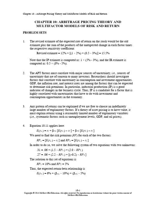
CHAPTER 10: ARBITRAGE PRICING THEORY ANDMULTIFACTOR MODELS OF RISK AND RETURN PROBLEM SETS1. The revised estimate of the expected rate of return on the stock would be the oldestimate plus the sum of the products of the unexpected change in each factor times the respective sensitivity coefficient:Revised estimate = 12% + [(1 × 2%) + (0.5 × 3%)] = 15.5%Note that the IP estimate is computed as: 1 × (5% - 3%), and the IR estimate iscomputed as: 0.5 × (8% - 5%).2. The APT factors must correlate with major sources of uncertainty, i.e., sources ofuncertainty that are of concern to many investors. Researchers should investigatefactors that correlate with uncertainty in consumption and investment opportunities.GDP, the inflation rate, and interest rates are among the factors that can be expected to determine risk premiums. In particular, industrial production (IP) is a goodindicator of changes in the business cycle. Thus, IP is a candidate for a factor that is highly correlated with uncertainties that have to do with investment andconsumption opportunities in the economy.3. Any pattern of returns can be explained if we are free to choose an indefinitelylarge number of explanatory factors. If a theory of asset pricing is to have value, itmust explain returns using a reasonably limited number of explanatory variables(i.e., systematic factors such as unemployment levels, GDP, and oil prices).4. Equation 10.11 applies here:E(r p) = r f + βP1 [E(r1 ) −r f ] + βP2 [E(r2 ) – r f]We need to find the risk premium (RP) for each of the two factors:RP1 = [E(r1 ) −r f] and RP2 = [E(r2 ) −r f]In order to do so, we solve the following system of two equations with two unknowns: .31 = .06 + (1.5 ×RP1 ) + (2.0 ×RP2 ).27 = .06 + (2.2 ×RP1 ) + [(–0.2) ×RP2 ]The solution to this set of equations isRP1 = 10% and RP2 = 5%Thus, the expected return-beta relationship isE(r P) = 6% + (βP1× 10%) + (βP2× 5%)5. The expected return for portfolio F equals the risk-free rate since its beta equals 0.For portfolio A, the ratio of risk premium to beta is (12 − 6)/1.2 = 5For portfolio E, the ratio is lower at (8 – 6)/0.6 = 3.33This implies that an arbitrage opportunity exists. For instance, you can create aportfolio G with beta equal to 0.6 (the same as E’s) by combining portfolio A and portfolio F in equal weights. The expected return and beta for portfolio G are then: E(r G) = (0.5 × 12%) + (0.5 × 6%) = 9%βG = (0.5 × 1.2) + (0.5 × 0%) = 0.6Comparing portfolio G to portfolio E, G has the same beta and higher return.Therefore, an arbitrage opportunity exists by buying portfolio G and selling anequal amount of portfolio E. The profit for this arbitrage will ber G – r E =[9% + (0.6 ×F)] − [8% + (0.6 ×F)] = 1%That is, 1% of the funds (long or short) in each portfolio.6. Substituting the portfolio returns and betas in the expected return-beta relationship,we obtain two equations with two unknowns, the risk-free rate (r f) and the factor risk premium (RP):12% = r f + (1.2 ×RP)9% = r f + (0.8 ×RP)Solving these equations, we obtainr f = 3% and RP = 7.5%7. a. Shorting an equally weighted portfolio of the ten negative-alpha stocks andinvesting the proceeds in an equally-weighted portfolio of the 10 positive-alpha stocks eliminates the market exposure and creates a zero-investmentportfolio. Denoting the systematic market factor as R M, the expected dollarreturn is (noting that the expectation of nonsystematic risk, e, is zero):$1,000,000 × [0.02 + (1.0 ×R M)] − $1,000,000 × [(–0.02) + (1.0 ×R M)]= $1,000,000 × 0.04 = $40,000The sensitivity of the payoff of this portfolio to the market factor is zerobecause the exposures of the positive alpha and negative alpha stocks cancelout. (Notice that the terms involving R M sum to zero.) Thus, the systematiccomponent of total risk is also zero. The variance of the analyst’s profit is notzero, however, since this portfolio is not well diversified.For n = 20 stocks (i.e., long 10 stocks and short 10 stocks) the investor willhave a $100,000 position (either long or short) in each stock. Net marketexposure is zero, but firm-specific risk has not been fully diversified. Thevariance of dollar returns from the positions in the 20 stocks is20 × [(100,000 × 0.30)2] = 18,000,000,000The standard deviation of dollar returns is $134,164.b. If n = 50 stocks (25 stocks long and 25 stocks short), the investor will have a$40,000 position in each stock, and the variance of dollar returns is50 × [(40,000 × 0.30)2] = 7,200,000,000The standard deviation of dollar returns is $84,853.Similarly, if n = 100 stocks (50 stocks long and 50 stocks short), the investorwill have a $20,000 position in each stock, and the variance of dollar returns is100 × [(20,000 × 0.30)2] = 3,600,000,000The standard deviation of dollar returns is $60,000.Notice that, when the number of stocks increases by a factor of 5 (i.e., from 20 to 100), standard deviation decreases by a factor of 5= 2.23607 (from$134,164 to $60,000).8. a. )(σσβσ2222e M +=88125)208.0(σ2222=+×=A50010)200.1(σ2222=+×=B97620)202.1(σ2222=+×=Cb. If there are an infinite number of assets with identical characteristics, then awell-diversified portfolio of each type will have only systematic risk since thenonsystematic risk will approach zero with large n. Each variance is simply β2 × market variance:222Well-diversified σ256Well-diversified σ400Well-diversified σ576A B C;;;The mean will equal that of the individual (identical) stocks.c. There is no arbitrage opportunity because the well-diversified portfolios allplot on the security market line (SML). Because they are fairly priced, there isno arbitrage.9. a. A long position in a portfolio (P) composed of portfolios A and B will offer anexpected return-beta trade-off lying on a straight line between points A and B.Therefore, we can choose weights such that βP = βC but with expected returnhigher than that of portfolio C. Hence, combining P with a short position in Cwill create an arbitrage portfolio with zero investment, zero beta, and positiverate of return.b. The argument in part (a) leads to the proposition that the coefficient of β2must be zero in order to preclude arbitrage opportunities.10. a. E(r) = 6% + (1.2 × 6%) + (0.5 × 8%) + (0.3 × 3%) = 18.1%b.Surprises in the macroeconomic factors will result in surprises in the return ofthe stock:Unexpected return from macro factors =[1.2 × (4% – 5%)] + [0.5 × (6% – 3%)] + [0.3 × (0% – 2%)] = –0.3%E(r) =18.1% − 0.3% = 17.8%11. The APT required (i.e., equilibrium) rate of return on the stock based on r f and thefactor betas isRequired E(r) = 6% + (1 × 6%) + (0.5 × 2%) + (0.75 × 4%) = 16% According to the equation for the return on the stock, the actually expected return on the stock is 15% (because the expected surprises on all factors are zero bydefinition). Because the actually expected return based on risk is less than theequilibrium return, we conclude that the stock is overpriced.12. The first two factors seem promising with respect to the likely impact on the firm’scost of capital. Both are macro factors that would elicit hedging demands acrossbroad sectors of investors. The third factor, while important to Pork Products, is a poor choice for a multifactor SML because the price of hogs is of minor importance to most investors and is therefore highly unlikely to be a priced risk factor. Betterchoices would focus on variables that investors in aggregate might find moreimportant to their welfare. Examples include: inflation uncertainty, short-terminterest-rate risk, energy price risk, or exchange rate risk. The important point here is that, in specifying a multifactor SML, we not confuse risk factors that are important toa particular investor with factors that are important to investors in general; only the latter are likely to command a risk premium in the capital markets.13. The formula is ()0.04 1.250.08 1.50.02.1717%E r =+×+×==14. If 4%f r = and based on the sensitivities to real GDP (0.75) and inflation (1.25),McCracken would calculate the expected return for the Orb Large Cap Fund to be:()0.040.750.08 1.250.02.040.0858.5% above the risk free rate E r =+×+×=+=Therefore, Kwon’s fundamental analysis estimate is congruent with McCracken’sAPT estimate. If we assume that both Kwon and McCracken’s estimates on the return of Orb’s Large Cap Fund are accurate, then no arbitrage profit is possible.15. In order to eliminate inflation, the following three equations must be solvedsimultaneously, where the GDP sensitivity will equal 1 in the first equation,inflation sensitivity will equal 0 in the second equation and the sum of the weights must equal 1 in the third equation.1.1.250.75 1.012.1.5 1.25 2.003.1wx wy wz wz wy wz wx wy wz ++=++=++=Here, x represents Orb’s High Growth Fund, y represents Large Cap Fund and z represents Utility Fund. Using algebraic manipulation will yield wx = wy = 1.6 and wz = -2.2.16. Since retirees living off a steady income would be hurt by inflation, this portfoliowould not be appropriate for them. Retirees would want a portfolio with a return positively correlated with inflation to preserve value, and less correlated with the variable growth of GDP. Thus, Stiles is wrong. McCracken is correct in that supply side macroeconomic policies are generally designed to increase output at aminimum of inflationary pressure. Increased output would mean higher GDP, which in turn would increase returns of a fund positively correlated with GDP.17. The maximum residual variance is tied to the number of securities (n ) in theportfolio because, as we increase the number of securities, we are more likely to encounter securities with larger residual variances. The starting point is todetermine the practical limit on the portfolio residual standard deviation, σ(e P ), that still qualifies as a well-diversified portfolio. A reasonable approach is to compareσ2(e P) to the market variance, or equivalently, to compare σ(e P) to the market standard deviation. Suppose we do not allow σ(e P) to exceed pσM, where p is a small decimal fraction, for example, 0.05; then, the smaller the value we choose for p, the more stringent our criterion for defining how diversified a well-diversified portfolio must be.Now construct a portfolio of n securities with weights w1, w2,…,w n, so that Σw i =1. The portfolio residual variance is σ2(e P) = Σw12σ2(e i)To meet our practical definition of sufficiently diversified, we require this residual variance to be less than (pσM)2. A sure and simple way to proceed is to assume the worst, that is, assume that the residual variance of each security is the highest possible value allowed under the assumptions of the problem: σ2(e i) = nσ2MIn that case σ2(e P) = Σw i2 nσM2Now apply the constraint: Σw i2 nσM2 ≤ (pσM)2This requires that: nΣw i2 ≤ p2Or, equivalently, that: Σw i2 ≤ p2/nA relatively easy way to generate a set of well-diversified portfolios is to use portfolio weights that follow a geometric progression, since the computations then become relatively straightforward. Choose w1 and a common factor q for the geometric progression such that q < 1. Therefore, the weight on each stock is a fraction q of the weight on the previous stock in the series. Then the sum of n terms is:Σw i= w1(1– q n)/(1– q) = 1or: w1 = (1– q)/(1– q n)The sum of the n squared weights is similarly obtained from w12 and a common geometric progression factor of q2. ThereforeΣw i2 = w12(1– q2n)/(1– q 2)Substituting for w1 from above, we obtainΣw i2 = [(1– q)2/(1– q n)2] × [(1– q2n)/(1– q 2)]For sufficient diversification, we choose q so that Σw i2 ≤ p2/nFor example, continue to assume that p = 0.05 and n = 1,000. If we chooseq = 0.9973, then we will satisfy the required condition. At this value for q w1 = 0.0029 and w n = 0.0029 × 0.99731,000In this case, w1 is about 15 times w n. Despite this significant departure from equal weighting, this portfolio is nevertheless well diversified. Any value of q between0.9973 and 1.0 results in a well-diversified portfolio. As q gets closer to 1, theportfolio approaches equal weighting.18. a. Assume a single-factor economy, with a factor risk premium E M and a (large)set of well-diversified portfolios with beta βP. Suppose we create a portfolio Zby allocating the portion w to portfolio P and (1 – w) to the market portfolioM. The rate of return on portfolio Z is:R Z = (w × R P) + [(1 – w) × R M]Portfolio Z is riskless if we choose w so that βZ = 0. This requires that:βZ = (w × βP) + [(1 – w) × 1] = 0 ⇒w = 1/(1 – βP) and (1 – w) = –βP/(1 – βP)Substitute this value for w in the expression for R Z:R Z = {[1/(1 – βP)] × R P} – {[βP/(1 – βP)] × R M}Since βZ = 0, then, in order to avoid arbitrage, R Z must be zero.This implies that: R P = βP × R MTaking expectations we have:E P = βP × E MThis is the SML for well-diversified portfolios.b. The same argument can be used to show that, in a three-factor model withfactor risk premiums E M, E1 and E2, in order to avoid arbitrage, we must have:E P = (βPM × E M) + (βP1 × E1) + (βP2 × E2)This is the SML for a three-factor economy.19. a. The Fama-French (FF) three-factor model holds that one of the factors drivingreturns is firm size. An index with returns highly correlated with firm size (i.e.,firm capitalization) that captures this factor is SMB (small minus big), thereturn for a portfolio of small stocks in excess of the return for a portfolio oflarge stocks. The returns for a small firm will be positively correlated withSMB. Moreover, the smaller the firm, the greater its residual from the othertwo factors, the market portfolio and the HML portfolio, which is the returnfor a portfolio of high book-to-market stocks in excess of the return for aportfolio of low book-to-market stocks. Hence, the ratio of the variance of thisresidual to the variance of the return on SMB will be larger and, together withthe higher correlation, results in a high beta on the SMB factor.b.This question appears to point to a flaw in the FF model. The model predictsthat firm size affects average returns so that, if two firms merge into a largerfirm, then the FF model predicts lower average returns for the merged firm.However, there seems to be no reason for the merged firm to underperformthe returns of the component companies, assuming that the component firmswere unrelated and that they will now be operated independently. We mighttherefore expect that the performance of the merged firm would be the sameas the performance of a portfolio of the originally independent firms, but theFF model predicts that the increased firm size will result in lower averagereturns. Therefore, the question revolves around the behavior of returns for aportfolio of small firms, compared to the return for larger firms that resultfrom merging those small firms into larger ones. Had past mergers of smallfirms into larger firms resulted, on average, in no change in the resultantlarger firms’ stock return characteristics (compared to the portfolio of stocksof the merged firms), the size factor in the FF model would have failed.Perhaps the reason the size factor seems to help explain stock returns is that,when small firms become large, the characteristics of their fortunes (andhence their stock returns) change in a significant way. Put differently, stocksof large firms that result from a merger of smaller firms appear empirically tobehave differently from portfolios of the smaller component firms.Specifically, the FF model predicts that the large firm will have a smaller riskpremium. Notice that this development is not necessarily a bad thing for thestockholders of the smaller firms that merge. The lower risk premium may bedue, in part, to the increase in value of the larger firm relative to the mergedfirms.CFA PROBLEMS1. a. This statement is incorrect. The CAPM requires a mean-variance efficientmarket portfolio, but APT does not.b.This statement is incorrect. The CAPM assumes normally distributed securityreturns, but APT does not.c. This statement is correct.2. b. Since portfolio X has β = 1.0, then X is the market portfolio and E(R M) =16%.Using E(R M ) = 16% and r f = 8%, the expected return for portfolio Y is notconsistent.3. d.4. c.5. d.6. c. Investors will take on as large a position as possible only if the mispricingopportunity is an arbitrage. Otherwise, considerations of risk anddiversification will limit the position they attempt to take in the mispricedsecurity.7. d.8. d.。
投资学10~12课后习题

出现错误,而当出现这种失误操作时,通常感到非常难过和悲哀。所以,投资者 在投资过程中, 为了避免后悔心态的出现,经常会表现出一种优柔寡断的性格特 点。 投资者在决定是否卖出一只股票时,往往受到买入时的成本比现价高或是低 的情绪影响,由于害怕后悔而想方设法尽量避免后悔的发生。有研究者认为:投 资者不愿卖出已下跌的股票,是为了避免作了一次失败投资的痛苦和后悔心情, 向其他人报告投资亏损的难堪也使其不愿去卖出已亏损的股票。 另一些研究者认 为: 投资者的从众行为和追随常识,是为了避免由于做出了一个错误的投资决定 而后悔。许多投资者认为:买一只大家都看好的股票比较容易,因为大家都看好 它并且买了它,即使股价下跌也没什么。大家都错了,所以我错了也没什么!而 如果自作主张买了一只市场形象不佳的股票,如果买人之后它就下跌, 自己就 很难合理地解释当时买它的理由。此外,基金经理人和股评家喜欢名气大的上市 公司股票, 主要原因也是因为如果这些股票下跌,他们因为操作得不好而被解雇 的可能性较小。害怕后悔也反映了投资者对自我的一种期望。Hersh Shefrin 和 Meir Statman 在一个研究中发现:投资者在投资过程中除了避免后悔以外,还 有一种追求自豪的动机在起作用。 害怕后悔与追求自豪造成了投资者持有获利股 票的时间太短,而持有亏损股票的时间太长。他们称这种现象为卖出效应。他们 发现:当投资者持有两只股票,股票 A 获利 20 ,而股票 B 亏损 20% ,此时又有 一个新的投资机会,而投资者由于没有别的钱,必需先卖掉一只股票时,多数投 资者往往卖掉股票 A 而不是股票 B。因为卖出股票 B 会对从前的买人决策后悔, 而卖出股票 A 会让投资者有一种做出正确投资的自豪感。 b.预测错误 c.心理账户:心理账户的存在影响着人们以不同的态度对待不同的支出和收益, 从而做出不同的决策和行为。 在上面的问题中,抛售掉的股票亏损和没有被抛掉 的股票亏损就是被放在不同的心理账户中,抛售之前是账面上的亏损,而抛售之 后是一个实际的亏损,客观上讲,这两者实质上并没有差异,但是在心理上人们 却把它们划上了严格的界限。 从账面亏损到实际亏损,后者在心理账户中感觉更 加“真实” ,也就更加让人痛苦,所以这两个账户给人的感觉是不同的,人们并 不能从心理上把二者完全等同起来。 当原来的账面亏损不小心成了实际亏损之后, 那个股票的账面亏损账户在心里就以最终亏损的状态关闭了, 人们一般不能把账
投资学课后习题及答案

投资学课后习题及答案投资学课后习题及答案投资学练习导论习题1证券投资是指投资者购买_______、________、________等有价证券以及这些有价证券的_______以获取________、_________及________的投资行为和投资过程,是直接投资的重要形式。
(填空)2 ____是投资者为实现投资目标所遵循的基本方针和基本准则。
(单选) A证券投资政策 B证券投资分析 C证券投组合 D评估证券投资组合的业绩3 一般来说,证券投资与投机的区别主要可以从________等不同角度进行分析。
(多选) A 动机 B对证券所作的分析方法 C投资期限 D投资对象E风险倾向4在证券市场中,难免出现投机行为,有投资就必然有投机。
适度的投机有利于证券市场发展(判断)第一至第四章习题1在股份有限公司利润增长时,参与优先股股东除了按固定股息率取得股息外,还可以分得___________。
(填空)2 累积优先股是一种常见的、发行很广泛的优先股股票。
其特点是股息率______,而且可以 ________计算。
(填空)3________不是优先股的特征之一。
(单选)A约定股息率 B股票可由公司赎回 C具有表决权 D优先分派股息和清偿剩余资产。
4 股份有限公司最初发行的大多是_____,通过这类股票所筹集的资金通常是股份有限公司股本的基础。
(单选) A特别股 B优先股 CB股 D普通股5 当公司前景和股市行情看好、盈利增加时,可转换优先股股东的最佳策略是_______ 。
(单选)A转换成参与优先股 B转换成公司债券 C转换成普通股 D转换成累积优先股6 下列外资股中,不属于境外上市外资股的是________。
(单选)A H股 BN股 CB股 DS股7 股份制就是以股份公司为核心,以股票发行为基础,以股票交易为依托。
(判断) 8 可赎回优先股是指允许拥有该股票的股东在一个合理的价格范围内将资金赎回。
(判断) 9________是指在管理层和股东之间发生冲突的可能性,它是由管理层在利益回报方面的控制以及管理人员的低效业绩所产生的问题。
- 1、下载文档前请自行甄别文档内容的完整性,平台不提供额外的编辑、内容补充、找答案等附加服务。
- 2、"仅部分预览"的文档,不可在线预览部分如存在完整性等问题,可反馈申请退款(可完整预览的文档不适用该条件!)。
- 3、如文档侵犯您的权益,请联系客服反馈,我们会尽快为您处理(人工客服工作时间:9:00-18:30)。
讼获得的异常收益 3%。但是按理来讲公司赢得了 500 万,其收益应该为 5%, 而在实际收益率中仅仅显示了 3%的收益,这一点很奇怪,难道是因为预期过 高? 22.这种策略表面上可以展示最佳的购买时间,但是实际上,这种策略与技术分 析的思路很像, 通过历史数据和趋势来预测未来的价格, 如果市场是有效的, 那么市场中的信息全部都反映在了股票价格之中,不能通过技术分析获得超 额收益,鉴于目前的市场并非完全有效,对于那些勤奋的、眼光独到的投资 者,仍然能通过技术分析、信息搜寻找到被低估的股票,以及某些趋势,并 且能够把握趋势的度 23.因为这些精准的预测信息已经反映在股票的价格之中了,一旦预测到经济将 要复苏,那么股票的价格会立即上扬,人们来不及出手,股票价格就已经上 升并稳定了 24.我会买入该只股票,因为它的实际价值比市场估计的价值要高 25.福特新车型会非常受市场欢迎,因而会大卖,那么这一利好消息将会反映在 股价中,股票价格会上涨
5. 有效市场假说的支持者认为市场是有效的,不能通过市场上的信息来获取超 额收益,所以积极投资是无效的,消极投资(指数投资策略)更优;行为金 融学派的支持者认为套利活动是不存在的, 但是这不一定代表市场是有效的, 而是套利活动被某些因素限制了,所以才导致了消极策略更优 6. A 7. A 8. B 9. 43512 10.基本面风险是指虽然投资者知道一个可以盈利的信息或者机会,但是这个机 会并非是无风险的,而这种风险可能突破了投资者能承受的底线。基本面风 险的存在限制了套利机会,导致行为偏差继续存在 11.数据挖掘是指投资者对于过去股票价格和成交量数据的观测与分析。数据挖 掘会使投资者发现实际上并不存在的股票走势模型,所以技术人员要非常小 心使用这些模型 12.价格服从随机漫走,可能是由于收到某些因素的限制,而不一定是因为信息 有效。正如没有套利活动,不一定就是市场有效一样。信息有效能够让整个 市场透明,使得价格能真实地反映价值,从而让资源得到最有效的利用 23 和 24 题不会做 25.分散不足的基金,因为其面临的风险更大,很难对其进行套利,所以价格偏 离净资产价值的高 CFA 1.365 2.a.后悔规避:投资者在投资过程中常出现后悔的心理状态。在大牛市背景下, 没有及时介入自己看好的股票会后悔,过早卖出获利的股票也会后悔;在熊市 (bear market)背景下,没能及时止损出局会后悔,获点小利没能兑现,然后又 被套牢也会后悔;在平衡市场中,自己持有的股票不涨不跌,别人推荐的股票上 涨, 自己会因为没有听从别人的劝告而及时换股后悔;当下定决心,卖出手中 不涨的股票,而买入专家推荐的股票, 又发现自己原来持有的股票不断上涨, 而专家推荐的股票不涨反跌时,更加后悔。Santa Clara 大学的 Meir Statman 教授是研究“害怕后悔” 行为的专家。由于人们在投资判断和决策上经常容易
8. 不理解这句话到底是什么意思。 股票价格波动, 当然会有人获益, 有人赔损。 经营的很好的人就会长期平均获得正的收益 9. C 因为市场弱有效,说明市场上的信息是公开的,不存在通过公开的市场信 息而获利
10.A 11.C 如果获得超额收益,那说明能够从市场数据中分析出有用的信息 12.B 13.A 不正确 B 不正确 C 正确 14.D 15.不违反 16.不可以,这样违背了市场有效假说 17.A.不违背,可能是运气 B 违背,不可预测 C 不违背 D 违背 E 违背,不可预 测 18.-1.9% 19.3% 和 1% 20.预期两家公司的收益分别为 4.4%和 1.7%,但实际分别为 3.1%和 2.5%,所以 两家公司的异常收益分别为-1.3%和 0.8%,由此可以判断后者获得了胜利 21.A.8% B.7% C.原先的预期为 7%,而实际的收益为 10%,这因为赢得了诉
出现错误,而当出现这种失误操作时,通常感到非常难过和悲哀。所以,投资者 在投资过程中, 为了避免后悔心态的出现,经常会表现出一种优柔寡断的性格特 点。 投资者在决定是否卖出一只股票时,往往受到买入时的成本比现价高或是低 的情绪影响,由于害怕后悔而想方设法尽量避免后悔的发生。有研究者认为:投 资者不愿卖出已下跌的股票,是为了避免作了一次失败投资的痛苦和后悔心情, 向其他人报告投资亏损的难堪也使其不愿去卖出已亏损的股票。 另一些研究者认 为: 投资者的从众行为和追随常识,是为了避免由于做出了一个错误的投资决定 而后悔。许多投资者认为:买一只大家都看好的股票比较容易,因为大家都看好 它并且买了它,即使股价下跌也没什么。大家都错了,所以我错了也没什么!而 如果自作主张买了一只市场形象不佳的股票,如果买人之后它就下跌, 自己就 很难合理地解释当时买它的理由。此外,基金经理人和股评家喜欢名气大的上市 公司股票, 主要原因也是因为如果这些股票下跌,他们因为操作得不好而被解雇 的可能性较小。害怕后悔也反映了投资者对自我的一种期望。Hersh Shefrin 和 Meir Statman 在一个研究中发现:投资者在投资过程中除了避免后悔以外,还 有一种追求自豪的动机在起作用。 害怕后悔与追求自豪造成了投资者持有获利股 票的时间太短,而持有亏损股票的时间太长。他们称这种现象为卖出效应。他们 发现:当投资者持有两只股票,股票 A 获利 20 ,而股票 B 亏损 20% ,此时又有 一个新的投资机会,而投资者由于没有别的钱,必需先卖掉一只股票时,多数投 资者往往卖掉股票 A 而不是股票 B。因为卖出股票 B 会对从前的买人决策后悔, 而卖出股票 A 会让投资者有一种做出正确投资的自豪感。 b.预测错误 c.心理账户:心理账户的存在影响着人们以不同的态度对待不同的支出和收益, 从而做出不同的决策和行为。 在上面的问题中,抛售掉的股票亏损和没有被抛掉 的股票亏损就是被放在不同的心理账户中,抛售之前是账面上的亏损,而抛售之 后是一个实际的亏损,客观上讲,这两者实质上并没有差异,但是在心理上人们 却把它们划上了严格的界限。 从账面亏损到实际亏损,后者在心理账户中感觉更 加“真实” ,也就更加让人痛苦,所以这两个账户给人的感觉是不同的,人们并 不能从心理上把二者完全等同起来。 当原来的账面亏损不小心成了实际亏损之后, 那个股票的账面亏损账户在心里就以最终亏损的状态关闭了, 人们一般不能把账
第十二章 行为金融与技术分析 1. 行为偏差与技术分析对交易量数据的使用是一致的,当交易者过分自信的时 候,其交易可能较为频繁,从而导致成交量与市场收益之间的相关关系,因 此,技术分析通过历史价格和成交量来指导投资策略能够成功 2. 虽然许多投资者存在行为偏差,但是他们的错误定价可能被那些精明的投资 者发现,出现套利,最终导致市场价格回到真实价格水平,即市场还是有效 的 3. 基本面风险、执行成本、模型风险 4. 这里所说的行为偏差不影响资产的均衡价格,应该说的是长期资产价格会回 到均衡水平, 但是在短期内, 由于行为偏差的存在, 仍然会引起股价的波动, 以及错误定价,在短期内,由于每个人对风险的承受能力不一样,能承受的 成本也不一样,因而会有投资者关注应为偏差
第十一章 有效市场假说 1. 相关系数为 0 2. 没有,因为它的创造了相应的价值 3. 错误,公平定价是说不存在套利的机会,并不等于所有的证券的期望收益相 等 4. 没有,既然它是增长性的企业,那应该将股息留着用于投资,这样会为股东 创造更大的价值 5. 不会,这种事可能是运气 6. 不准确。变动性较强的股票的所有信息都会反映在股价中,所以不存在市场 不知如何定价这一说 7. 市盈率效应:资本市场均衡错在没有对收益进行调整。如果资本资产定价模 型用于估计基准业绩,市盈率将于异常收益相关 小公司效应:由于小公司通常被大的投资机构忽略,因而小公司的信息经常 难以获得
投资学课后习题 管实 1101 张娟 U201113738 第十章 套利定价理论与风险收益多因素模型 1.15.5% 2.其实研究者也不确定哪些因素决定了风险溢价, 他们采取的方法是不断的尝试, 首先是选取那些最能够反映宏观经济的因素,接着利用计量经济学中的方法,不 断做回归,选出那些性质好的因素。工业产值比较能反映宏观经济,并且回归的 解释力度高,所以选取了工业产值这个因素。 3.否则将会存在大量的套利机会 4.E = 6% + 10%β
26.相对比市场行情,该公司的年收益增长可能微不足道,或者说相对在下降 27.这并不违背,因为交易很少的小公司的很多信息很难获得,其承受的风险也 比较大,所以其获得正的α 也很正常 28.看不懂这个图,为什么会同时出现买入和卖出呢。这些买入和卖出是那些人 在操作,从图中我们看到,在消息公布之前,买入增加,卖出为负,在信息 公布之前,卖出突然大幅增加,买入大幅减少,在消息公布之后,买入大幅 增加,卖出大幅减小,并且最后两者趋于稳定。 29.A.不违背。有效市场假说的联系,不能说市场有效了,那风险便消失了。当经济处于萧 条时期,市场环境不好可能导致股价下跌,这个时候虽然有高的风险溢价, 但是其他的因素同样影响股价预期,比如无风险利率,敏感系数等 B.投资者非理性时会出现过度反应
1
+ 5%β
2
5.同投资组合 A 的数据算出的市场收益率为 11%,用公式算出投资组合 E 的期望 应为 9%, 但是这里 E 的期望仅为 8%, 说明存在一个投资组合, 与 E 有相同的β , 但是期望收益更高。可以将组合的一半投资于 A,一半投资于无风险资产,这样 便构造出了更优于 E 的投资组合 F,然后卖掉 E,买进 F,可获利 1%。 6.3% 7.a. 4 万美元,134164 美元 b.当股票只数由 20 变为 50,100 时,其标准差分别为 84843 美元,6 万美元 8.a.881,500,976 b. 若是完全分散的投资组合, 那只剩下系统风险, A 的方差为 256, B 的为 400, C 的为 576 c.三者的超额溢价比上β 的值分别为 12.5,12,11.67,所以市场上存在套利, 比如我们可以卖掉 B 和 C,然后通过投资 A 和无风险资产构造与之相等的β ,这 样便可以实现套利。 9.a.构建一个投资组合包含 A 和 B,这样我们可以得到在相同的β 下,收益率高 于投资组合 C,因而产生了套利。 b.从图形来看,可能与收益成比例。 10.a.18.1% b.17.8%