投资学10版习题答案CH18

合集下载

投资学10版习题答案CH18

投资学10版习题答案10

CHAPTER 10: ARBITRAGE PRICING THEORY ANDMULTIFACTOR MODELS OF RISK AND RETURN PROBLEM SETS1. The revised estimate of the expected rate of return on the stock would be the oldestimate plus the sum of the products of the unexpected change in each factor times the respective sensitivity coefficient:Revised estimate = 12% + [(1 × 2%) + (0.5 × 3%)] = 15.5%Note that the IP estimate is computed as: 1 × (5% - 3%), and the IR estimate iscomputed as: 0.5 × (8% - 5%).2. The APT factors must correlate with major sources of uncertainty, i.e., sources ofuncertainty that are of concern to many investors. Researchers should investigatefactors that correlate with uncertainty in consumption and investment opportunities.GDP, the inflation rate, and interest rates are among the factors that can be expected to determine risk premiums. In particular, industrial production (IP) is a goodindicator of changes in the business cycle. Thus, IP is a candidate for a factor that is highly correlated with uncertainties that have to do with investment andconsumption opportunities in the economy.3. Any pattern of returns can be explained if we are free to choose an indefinitely largenumber of explanatory factors. If a theory of asset pricing is to have value, it mustexplain returns using a reasonably limited number of explanatory variables (i.e.,systematic factors such as unemployment levels, GDP, and oil prices).4. Equation 10.11 applies here:E(r p) = r f + βP1 [E(r1 ) -r f ] + βP2 [E(r2 ) –r f]We need to find the risk premium (RP) for each of the two factors:RP1 = [E(r1 ) -r f] and RP2 = [E(r2 ) -r f]In order to do so, we solve the following system of two equations with two unknowns: .31 = .06 + (1.5 ×RP1 ) + (2.0 ×RP2 ).27 = .06 + (2.2 ×RP1 ) + [(–0.2) ×RP2 ]The solution to this set of equations isRP1 = 10% and RP2 = 5%Thus, the expected return-beta relationship isE(r P) = 6% + (βP1× 10%) + (βP2× 5%)5. The expected return for portfolio F equals the risk-free rate since its beta equals 0.For portfolio A, the ratio of risk premium to beta is (12 − 6)/1.2 = 5For portfolio E, the ratio is lower at (8 – 6)/0.6 = 3.33This implies that an arbitrage opportunity exists. For instance, you can create aportfolio G with beta equal to 0.6 (the same as E’s) by combining portfolio A andportfolio F in equal weights. The expected return and beta for portfolio G are then: E(r G) = (0.5 × 12%) + (0.5 × 6%) = 9%βG = (0.5 × 1.2) + (0.5 × 0%) = 0.6Comparing portfolio G to portfolio E, G has the same beta and higher return.Therefore, an arbitrage opportunity exists by buying portfolio G and selling an equal amount of portfolio E. The profit for this arbitrage will ber G–r E =[9% + (0.6 ×F)] - [8% + (0.6 ×F)] = 1%That is, 1% of the funds (long or short) in each portfolio.6. Substituting the portfolio returns and betas in the expected return-beta relationship,we obtain two equations with two unknowns, the risk-free rate (r f) and the factorrisk premium (RP):12% = r f + (1.2 ×RP)9% = r f + (0.8 ×RP)Solving these equations, we obtainr f = 3% and RP = 7.5%7. a. Shorting an equally weighted portfolio of the ten negative-alpha stocks andinvesting the proceeds in an equally-weighted portfolio of the 10 positive-alphastocks eliminates the market exposure and creates a zero-investment portfolio.Denoting the systematic market factor as R M, the expected dollar return is(noting that the expectation of nonsystematic risk, e, is zero):$1,000,000 × [0.02 + (1.0 ×R M)] - $1,000,000 × [(–0.02) + (1.0 ×R M)]= $1,000,000 × 0.04 = $40,000The sensitivity of the payoff of this portfolio to the market factor is zerobecause the exposures of the positive alpha and negative alpha stocks cancelout. (Notice that the terms involving R M sum to zero.) Thus, the systematiccomponent of total risk is also zero. The variance of the analyst’s profit is notzero, however, since this portfolio is not well diversified.For n = 20 stocks (i.e., long 10 stocks and short 10 stocks) the investor willhave a $100,000 position (either long or short) in each stock. Net marketexposure is zero, but firm-specific risk has not been fully diversified. Thevariance of dollar returns from the positions in the 20 stocks is20 × [(100,000 × 0.30)2] = 18,000,000,000The standard deviation of dollar returns is $134,164.b. If n = 50 stocks (25 stocks long and 25 stocks short), the investor will have a$40,000 position in each stock, and the variance of dollar returns is50 × [(40,000 × 0.30)2] = 7,200,000,000The standard deviation of dollar returns is $84,853.Similarly, if n = 100 stocks (50 stocks long and 50 stocks short), the investorwill have a $20,000 position in each stock, and the variance of dollar returns is100 × [(20,000 × 0.30)2] = 3,600,000,000The standard deviation of dollar returns is $60,000.Notice that, when the number of stocks increases by a factor of 5 (i.e., from 20 to 100), standard deviation decreases by a factor of 5= 2.23607 (from$134,164 to $60,000).8. a.)(σσβσ2222e M+= 88125)208.0(σ2222=+⨯=A50010)200.1(σ2222=+⨯=B 97620)202.1(σ2222=+⨯=Cb. If there are an infinite number of assets with identical characteristics, then awell-diversified portfolio of each type will have only systematic risk since thenonsystematic risk will approach zero with large n. E ach variance is simply β2× market variance:222Well-diversified σ256Well-diversified σ400Well-diversified σ576AB CThe mean will equal that of the individual (identical) stocks.c. There is no arbitrage opportunity because the well-diversified portfolios allplot on the security market line (SML). Because they are fairly priced, there isno arbitrage.9. a. A long position in a portfolio (P) composed of portfolios A and B will offer anexpected return-beta trade-off lying on a straight line between points A and B.Therefore, we can choose weights such that βP = βC but with expected returnhigher than that of portfolio C. Hence, combining P with a short position in Cwill create an arbitrage portfolio with zero investment, zero beta, and positiverate of return.b. The argument in part (a) leads to the proposition that the coefficient of β2 mustbe zero in order to preclude arbitrage opportunities.10. a. E(r) = 6% + (1.2 × 6%) + (0.5 × 8%) + (0.3 × 3%) = 18.1%b.Surprises in the macroeconomic factors will result in surprises in the return ofthe stock:Unexpected return from macro factors =[1.2 × (4% – 5%)] + [0.5 × (6% – 3%)] + [0.3 × (0% – 2%)] = –0.3%E(r) =18.1% − 0.3% = 17.8%11. The APT required (i.e., equilibrium) rate of return on the stock based on r f and thefactor betas isRequired E(r) = 6% + (1 × 6%) + (0.5 × 2%) + (0.75 × 4%) = 16% According to the equation for the return on the stock, the actually expected returnon the stock is 15% (because the expected surprises on all factors are zero bydefinition). Because the actually expected return based on risk is less than theequilibrium return, we conclude that the stock is overpriced.12. The first two factors seem promising with respect to the likely impact on the firm’scost of capital. Both are macro factors that would elicit hedging demands across broad sectors of investors. The third factor, while important to Pork Products, is a poorchoice for a multifactor SML because the price of hogs is of minor importance tomost investors and is therefore highly unlikely to be a priced risk factor. Betterchoices would focus on variables that investors in aggregate might find moreimportant to their welfare. Examples include: inflation uncertainty, short-terminterest-rate risk, energy price risk, or exchange rate risk. The important point here is that, in specifying a multifactor SML, we not confuse risk factors that are important toa particular investor with factors that are important to investors in general; only the latter are likely to command a risk premium in the capital markets.13. The formula is ()0.04 1.250.08 1.50.02.1717%E r =+⨯+⨯==14. If 4%f r = and based on the sensitivities to real GDP (0.75) and inflation (1.25),McCracken would calculate the expected return for the Orb Large Cap Fund to be:()0.040.750.08 1.250.02.040.0858.5% above the risk free rate E r =+⨯+⨯=+=Therefore, Kwon’s fundamental analysis estimate is congruent with McCracken’sAPT estimate. If we assume that both Kwon and McCracken’s estimates on the return of Orb’s Large Cap Fund are accurate, then no arbitrage profit is possible.15. In order to eliminate inflation, the following three equations must be solvedsimultaneously, where the GDP sensitivity will equal 1 in the first equation,inflation sensitivity will equal 0 in the second equation and the sum of the weights must equal 1 in the third equation.1.1.250.75 1.012.1.5 1.25 2.003.1wx wy wz wz wy wz wx wy wz ++=++=++=Here, x represents Orb’s High Growth Fund, y represents Large Cap Fund and z represents Utility Fund. Using algebraic manipulation will yield wx = wy = 1.6 and wz = -2.2.16. Since retirees living off a steady income would be hurt by inflation, this portfoliowould not be appropriate for them. Retirees would want a portfolio with a return positively correlated with inflation to preserve value, and less correlated with the variable growth of GDP. Thus, Stiles is wrong. McCracken is correct in that supply side macroeconomic policies are generally designed to increase output at aminimum of inflationary pressure. Increased output would mean higher GDP, which in turn would increase returns of a fund positively correlated with GDP.17. The maximum residual variance is tied to the number of securities (n ) in theportfolio because, as we increase the number of securities, we are more likely toencounter securities with larger residual variances. The starting point is to determine the practical limit on the portfolio residual standard deviation, σ(e P ), that stillqualifies as a well-diversified portfolio. A reasonable approach is to compareσ2(e P) to the market variance, or equivalently, to compare σ(e P) to the market standard deviation. Suppose we do not allow σ(e P) to exceed pσM, where p is a small decimal fraction, for example, 0.05; then, the smaller the value we choose for p, the more stringent our criterion for defining how diversified a well-diversified portfolio must be.Now construct a portfolio of n securities with weights w1, w2,…,w n, so that ∑w i =1. The portfolio residual variance is σ2(e P) = ∑w12σ2(e i)To meet our practical definition of sufficiently diversified, we require this residual variance to be less than (pσM)2. A sure and simple way to proceed is to assume the worst, that is, assume that the residual variance of each security is the highest possible value allowed under the assumptions of the problem: σ2(e i) = nσ2MIn that case σ2(e P) = ∑w i2 nσM2Now apply the constraint: ∑w i2 nσM2 ≤ (pσM)2This requires that: n∑w i2 ≤ p2Or, equivalently, that: ∑w i2 ≤ p2/nA relatively easy way to generate a set of well-diversified portfolios is to use portfolio weights that follow a geometric progression, since the computations then become relatively straightforward. Choose w1 and a common factor q for the geometric progression such that q < 1. Therefore, the weight on each stock is a fraction q of the weight on the previous stock in the series. Then the sum of n terms is: ∑w i= w1(1– q n)/(1– q) = 1or: w1 = (1– q)/(1–q n)The sum of the n squared weights is similarly obtained from w12 and a common geometric progression factor of q2. Therefore∑w i2 = w12(1– q2n)/(1– q 2)Substituting for w1 from above, we obtain∑w i2 = [(1– q)2/(1–q n)2] × [(1– q2n)/(1– q 2)]For sufficient diversification, we choose q so that ∑w i2 ≤ p2/nFor example, continue to assume that p = 0.05 and n = 1,000. If we chooseq = 0.9973, then we will satisfy the required condition. At this value for q w1 = 0.0029 and w n = 0.0029 × 0.99731,000In this case, w1 is about 15 times w n. Despite this significant departure from equal weighting, this portfolio is nevertheless well diversified. Any value of q between0.9973 and 1.0 results in a well-diversified portfolio. As q gets closer to 1, theportfolio approaches equal weighting.18. a. Assume a single-factor economy, with a factor risk premium E M and a (large)set of well-diversified portfolios with beta βP. Suppose we create a portfolio Zby allocating the portion w to portfolio P and (1 –w) to the market portfolio M.The rate of return on portfolio Z is:R Z = (w ×R P) + [(1 –w) ×R M]Portfolio Z is riskless if we choose w so that βZ = 0. This requires that:βZ = (w ×βP) + [(1 –w) × 1] = 0 ⇒w = 1/(1 –βP) and (1 –w) = –βP/(1 –βP)Substitute this value for w in the expression for R Z:R Z = {[1/(1 –βP)] ×R P} – {[βP/(1 –βP)] ×R M}Since βZ = 0, then, in order to avoid arbitrage, R Z must be zero.This implies that: R P = βP ×R MTaking expectations we have:E P = βP ×E MThis is the SML for well-diversified portfolios.b. The same argument can be used to show that, in a three-factor model withfactor risk premiums E M, E1 and E2, in order to avoid arbitrage, we must have:E P = (βPM ×E M) + (βP1 ×E1) + (βP2 ×E2)This is the SML for a three-factor economy.19. a. The Fama-French (FF) three-factor model holds that one of the factors drivingreturns is firm size. An index with returns highly correlated with firm size (i.e.,firm capitalization) that captures this factor is SMB (small minus big), thereturn for a portfolio of small stocks in excess of the return for a portfolio oflarge stocks. The returns for a small firm will be positively correlated withSMB. Moreover, the smaller the firm, the greater its residual from the othertwo factors, the market portfolio and the HML portfolio, which is the returnfor a portfolio of high book-to-market stocks in excess of the return for aportfolio of low book-to-market stocks. Hence, the ratio of the variance of thisresidual to the variance of the return on SMB will be larger and, together withthe higher correlation, results in a high beta on the SMB factor.b.This question appears to point to a flaw in the FF model. The model predictsthat firm size affects average returns so that, if two firms merge into a largerfirm, then the FF model predicts lower average returns for the merged firm.However, there seems to be no reason for the merged firm to underperformthe returns of the component companies, assuming that the component firmswere unrelated and that they will now be operated independently. We mighttherefore expect that the performance of the merged firm would be the sameas the performance of a portfolio of the originally independent firms, but theFF model predicts that the increased firm size will result in lower averagereturns. Therefore, the question revolves around the behavior of returns for aportfolio of small firms, compared to the return for larger firms that resultfrom merging those small firms into larger ones. Had past mergers of smallfirms into larger firms resulted, on average, in no change in the resultant largerfirms’ stock return characteristics (compared to the portfolio of stocks of themerged firms), the size factor in the FF model would have failed.Perhaps the reason the size factor seems to help explain stock returns is that,when small firms become large, the characteristics of their fortunes (and hencetheir stock returns) change in a significant way. Put differently, stocks of largefirms that result from a merger of smaller firms appear empirically to behavedifferently from portfolios of the smaller component firms. Specifically, theFF model predicts that the large firm will have a smaller risk premium. Noticethat this development is not necessarily a bad thing for the stockholders of thesmaller firms that merge. The lower risk premium may be due, in part, to theincrease in value of the larger firm relative to the merged firms.CFA PROBLEMS1. a. This statement is incorrect. The CAPM requires a mean-variance efficientmarket portfolio, but APT does not.b.This statement is incorrect. The CAPM assumes normally distributed securityreturns, but APT does not.c. This statement is correct.2. b. Since portfolio X has = 1.0, then X is the market portfolio and E(R M) =16%.Using E(R M ) = 16% and r f = 8%, the expected return for portfolio Y is notconsistent.3. d.4. c.5. d.6. c. Investors will take on as large a position as possible only if the mispricingopportunity is an arbitrage. Otherwise, considerations of risk anddiversification will limit the position they attempt to take in the mispricedsecurity.7. d.8. d.。

投资学（博迪）第10版课后习题答...

投资学（博迪）第10版课后习题答...CHAPTER 10: ARBITRAGE PRICING THEORY ANDMULTIFACTOR MODELS OF RISK AND RETURN PROBLEM SETS1. The revised estimate of the expected rate of return on the stock would be the oldestimate plus the sum of the products of the unexpected change in each factor times the respective sensitivity coefficient: Revised estimate = 12% + [(1 × 2%) + (0.5 × 3%)] = 15.5%Note that the IP estimate is computed as: 1 × (5% - 3%), and the IR estimate iscomputed as: 0.5 × (8% - 5%).2. The APT factors must correlate with major sources of uncertainty, i.e., sources ofuncertainty that are of concern to many investors. Researchers should investigatefactors that correlate with uncertainty in consumption and investment opportunities.GDP, the inflation rate, and interest rates are among the factors that can be expected to determine risk premiums. In particular, industrial production (IP) is a goodindicator of changes in the business cycle. Thus, IP is a candidate for a factor that is highly correlated with uncertainties that have to do with investment andconsumption opportunities in the economy.3. Any pattern of returns can be explained if we are free to choose an indefinitelylarge number of explanatory factors. If a theory of asset pricing is to have value, itmust explain returns using a reasonably limited number of explanatory variables(i.e., systematic factors such as unemployment levels, GDP, and oil prices).4. Equation 10.11 applies here:E(r p) = r f + βP1 [E(r1 ) ?r f ] + βP2 [E(r2 ) – r f]We need to find the risk premium (RP) for each of the two factors:RP1 = [E(r1 ) ?r f] and RP2 = [E(r2 ) ?r f]In order to do so, we solve the following system of two equations with two unknowns: .31 = .06 + (1.5 ×RP1 ) + (2.0 ×RP2 ).27 = .06 + (2.2 ×RP1 ) + [(–0.2) ×RP2 ]The solution to this set of equations isRP1 = 10% and RP2 = 5%Thus, the expected return-beta relationship isE(r P) = 6% + (βP1× 10%) + (βP2× 5%)5. The expected return for portfolio F equals the risk-free rate since its beta equals 0.For portfolio A, the ratio of risk premium to beta is (12 ?6)/1.2 = 5For portfolio E, the ratio is lower at (8 – 6)/0.6 = 3.33This implies that an arbitrage opportunity exists. For instance, you can create aportfolio G with beta equal to 0.6 (the same as E’s) by combining portfolio A and portfolio F in equal weights. The expected return and beta for portfolio G are then: E(r G) = (0.5 × 12%) + (0.5 × 6%) = 9%βG = (0.5 × 1.2) + (0.5 × 0%) = 0.6Comparing portfolio G to portfolio E, G has the same betaand higher return.Therefore, an arbitrage opportunity exists by buying portfolio G and selling anequal amount of portfolio E. The profit for this arbitrage will ber G –r E =[9% + (0.6 ×F)] ?[8% + (0.6 ×F)] = 1%That is, 1% of the funds (long or short) in each portfolio.6. Substituting the portfolio returns and betas in the expected return-beta relationship,we obtain two equations with two unknowns, the risk-free rate (r f) and the factor risk premium (RP):12% = r f + (1.2 ×RP)9% = r f + (0.8 ×RP)Solving these equations, we obtainr f = 3% and RP = 7.5%7. a. Shorting an equally weighted portfolio of the ten negative-alpha stocks andinvesting the proceeds in an equally-weighted portfolio of the 10 positive-alpha stocks eliminates the market exposure and creates a zero-investmentportfolio. Denoting the systematic market factor as R M, the expected dollarreturn is (noting that the expectation of nonsystematic risk, e, is zero):$1,000,000 × [0.02 + (1.0 ×R M)] ? $1,000,000 × [(–0.02) + (1.0 ×R M)]= $1,000,000 × 0.04 = $40,000The sensitivity of the payoff of this portfolio to the market factor is zerobecause the exposures of the positive alpha and negative alpha stocks cancelout. (Notice that the terms involving R M sum to zero.) Thus, the systematiccomponent of total risk is also zero. The variance of the analyst’s profit is notzero, however, since this portfolio is not well diversified.For n = 20 stocks (i.e., long 10 stocks and short 10 stocks) the investor willhave a $100,000 position (either long or short) in each stock. Net marketexposure is zero, but firm-specific risk has not been fully diversified. Thevariance of dollar returns from the positions in the 20 stocks is20 × [(100,000 × 0.30)2] = 18,000,000,000The standard deviation of dollar returns is $134,164.b. If n = 50 stocks (25 stocks long and 25 stocks short), the investor will have a$40,000 position in each stock, and the variance of dollar returns is50 × [(40,000 × 0.30)2] = 7,200,000,000The standard deviation of dollar returns is $84,853.Similarly, if n = 100 stocks (50 stocks long and 50 stocks short), the investorwill have a $20,000 position in each stock, and the variance of dollar returns is100 × [(20,000 × 0.30)2] = 3,600,000,000The standard deviation of dollar returns is $60,000.Notice that, when the number of stocks increases by a factorof 5 (i.e., from 20 to 100), standard deviation decreases by a factor of 5= 2.23607 (from$134,164 to $60,000).8. a. )(σσβσ2222e M +=88125)208.0(σ2222=+×=A50010)200.1(σ2222=+×=B97620)202.1(σ2222=+×=Cb. If there are an infinite number of assets with identical characteristics, then awell-diversified portfolio of each type will have only systematic risk since thenonsystematic risk will approach zero with large n. Each variance is simply β2 × market variance:222Well-diversified σ256Well-diversified σ400Well-diversified σ576A B C;;;The mean will equal that of the individual (identical) stocks.c. There is no arbitrage opportunity because the well-diversified portfolios allplot on the security market line (SML). Because they are fairly priced, there isno arbitrage.9. a. A long position in a portfolio (P) composed of portfoliosA andB will offer anexpected return-beta trade-off lying on a straight linebetween points A and B.Therefore, we can choose weights such that βP = βC but with expected returnhigher than that of portfolio C. Hence, combining P with a short position in Cwill create an arbitrage portfolio with zero investment, zero beta, and positiverate of return.b. The argument in part (a) leads to the proposition that the coefficient of β2must be zero in order to preclude arbitrage opportunities.10. a. E(r) = 6% + (1.2 × 6%) + (0.5 × 8%) + (0.3 × 3%) = 18.1%b.Surprises in the macroeconomic factors will result in surprises in the return ofthe stock:Unexpected return from macro factors =[1.2 × (4% –5%)] + [0.5 × (6% –3%)] + [0.3 × (0% – 2%)] = –0.3%E(r) =18.1% ? 0.3% = 17.8%11. The APT required (i.e., equilibrium) rate of return on the stock based on r f and thefactor betas isRequired E(r) = 6% + (1 × 6%) + (0.5 × 2%) + (0.75 × 4%) = 16% According to the equation for the return on the stock, the actually expected return on the stock is 15% (because the expected surprises on all factors are zero bydefinition). Because the actually expected return based on risk is less than theequilibrium return, we conclude that the stock is overpriced.12. The first two factors seem promising with respect to thelikely impact on the firm’scost of capital. Both are macro factors that would elicit hedging demands acrossbroad sectors of investors. The third factor, while important to Pork Products, is a poor choice for a multifactor SML because the price of hogs is of minor importance to most investors and is therefore highly unlikely to be a priced risk factor. Better choices would focus on variables that investors in aggregate might find moreimportant to their welfare. Examples include: inflation uncertainty, short-terminterest-rate risk, energy price risk, or exchange rate risk. The important point here is that, in specifying a multifactor SML, we not confuse risk factors that are important toa particular investor with factors that are important to investors in general; only the latter are likely to command a risk premium in the capital markets.13. The formula is ()0.04 1.250.08 1.50.02.1717%E r =+×+×==14. If 4%f r = and based on the sensitivities to real GDP (0.75) and inflation (1.25),McCracken would calculate the expected return for the Orb Large Cap Fund to be:()0.040.750.08 1.250.02.040.0858.5% above the risk free rate E r =+×+×=+=Therefore, Kwon’s fundamental analysis estimate is congruent with McCr acken’sAPT estimate. If we assume that both Kwon and McCracken’s estimates on the return of Orb’s Large Cap Fund are accurate, then no arbitrage profit is possible.15. In order to eliminate inflation, the following three equations must be solvedsimultaneously, where the GDP sensitivity will equal 1 in the first equation,inflation sensitivity will equal 0 in the second equation and the sum of the weights must equal 1 in the third equation.1.1.250.75 1.012.1.5 1.25 2.003.1wx wy wz wz wy wz wx wy wz ++=++=++=Here, x represents Orb’s High Growth Fund, y represents Large Cap Fund and z represents Utility Fund. Using algebraic manipulation will yield wx = wy = 1.6 and wz = -2.2.16. Since retirees living off a steady income would be hurt by inflation, this portfoliowould not be appropriate for them. Retirees would want a portfolio with a return positively correlated with inflation to preserve value, and less correlated with the variable growth of GDP. Thus, Stiles is wrong. McCracken is correct in that supply side macroeconomic policies are generally designed to increase output at aminimum of inflationary pressure. Increased output would mean higher GDP, which in turn would increase returns of a fund positively correlated with GDP.17. The maximum residual variance is tied to the number of securities (n ) in theportfolio because, as we increase the number of securities, we are more likely to encounter securities with larger residual variances. The starting point is todetermine the practical limit on the portfolio residualstandard deviation, σ(e P ), that still qualifies as a well-diversified portfolio. A reasonable approach is to compareσ2(e P) to the market variance, or equivalently, to compare σ(e P) to the market standard deviation. Suppose we do n ot allow σ(e P) to exceed pσM, where p is a small decimal fraction, for example, 0.05; then, the smaller the value we choose for p, the more stringent our criterion for defining how diversified a well-diversified portfolio must be.Now construct a portfolio of n securities with weights w1, w2,…,w n, so that Σw i =1. The portfolio residual variance is σ2(e P) = Σw12σ2(e i)To meet our practical definition of sufficiently diversified, we require this residual variance to be less than (pσM)2. A sure and simple way to proceed is to assume the worst, that is, assume that the residual variance of each security is the highest possible value allowed under the assumptions of the problem: σ2(e i) = nσ2MIn that case σ2(e P) = Σw i2 nσM2Now apply the constraint: Σw i2nσM2 ≤ (pσM)2This requires that: nΣw i2 ≤ p2Or, equivalently, that: Σw i2 ≤ p2/nA relatively easy way to generate a set of well-diversified portfolios is to use portfolio weights that follow a geometric progression, since the computations then become relatively straightforward. Choose w1 and a common factor q for the geometric progression such that q < 1. Therefore, the weight on each stock is a fraction q of the weight on the previous stock in the series. Then the sum of n terms is:Σw i= w1(1– q n)/(1– q) = 1or: w1 = (1– q)/(1– q n)The sum of the n squared weights is similarly obtained from w12 and a common geometric progression factor of q2. ThereforeΣw i2 = w12(1– q2n)/(1– q 2)Substituting for w1 from above, we obtainΣw i2 = [(1– q)2/(1– q n)2] × [(1– q2n)/(1– q 2)]For sufficient diversification, we choose q so that Σw i2 ≤ p2/nFor example, continue to assume that p = 0.05 and n = 1,000. If we chooseq = 0.9973, then we will satisfy the required condition. At this value for q w1 = 0.0029 and w n = 0.0029 × 0.99731,000 In this case, w1 is about 15 times w n. Despite this significant departure from equal weighting, this portfolio is nevertheless well diversified. Any value of q between0.9973 and 1.0 results in a well-diversified portfolio. As q gets closer to 1, theportfolio approaches equal weighting.18. a. Assume a single-factor economy, with a factor risk premium E M and a (large)set of well-diversified portfolios with beta βP. Suppose we create a portfolio Zby allocating the portion w to portfolio P and (1 – w) to the market portfolioM. The rate of return on portfolio Z is:R Z = (w × R P) + [(1 –w) × R M]Portfolio Z is riskless if we choose w so that βZ = 0. This requires that:βZ = (w × βP) + [(1 –w) × 1] = 0 ?w = 1/(1 –βP) and (1 – w) = –βP/(1 –βP)Substitute this value for w in the expression for R Z:R Z = {[1/(1 –βP)] × R P} –{[βP/(1 –βP)] × R M}Since βZ = 0, then, in order to avoid arbitrage, R Z must be zero.This implies that: R P = βP × R MTaking expectations we have:E P = βP × E MThis is the SML for well-diversified portfolios.b. The same argument can be used to show that, in a three-factor model withfactor risk premiums E M, E1 and E2, in order to avoid arbitrage, we must have:E P = (βPM × E M) + (βP1 × E1) + (βP2 × E2)This is the SML for a three-factor economy.19. a. The Fama-French (FF) three-factor model holds that one of the factors drivingreturns is firm size. An index with returns highly correlated with firm size (i.e.,firm capitalization) that captures this factor is SMB (small minus big), thereturn for a portfolio of small stocks in excess of the return for a portfolio oflarge stocks. The returns for a small firm will be positively correlated withSMB. Moreover, the smaller the firm, the greater its residual from the othertwo factors, the market portfolio and the HML portfolio, which is the returnfor a portfolio of high book-to-market stocks in excess of the return for aportfolio of low book-to-market stocks. Hence, the ratio of the variance of thisresidual to the variance of the return on SMB will be larger and, together withthe higher correlation, results in a high beta on the SMB factor.b.This question appears to point to a flaw in the FF model. The model predictsthat firm size affects average returns so that, if two firms merge into a largerfirm, then the FF model predicts lower average returns for the merged firm.However, there seems to be no reason for the merged firm to underperformthe returns of the component companies, assuming that the component firmswere unrelated and that they will now be operated independently. We mighttherefore expect that the performance of the merged firm would be the sameas the performance of a portfolio of the originally independent firms, but theFF model predicts that the increased firm size will result in lower averagereturns. Therefore, the question revolves around the behavior of returns for aportfolio of small firms, compared to the return for larger firms that resultfrom merging those small firms into larger ones. Had past mergers of smallfirms into larger firms resulted, on average, in no change in the resultantlarger firms’ stock return characteristics (compared to the portfolio of stocksof the merged firms), the size factor in the FF model would have failed.Perhaps the reason the size factor seems to help explain stock returns is that,when small firms become large, the characteristics of their fortunes (andhence their stock returns) change in a significant way. Put differently, stocksof large firms that result from a merger of smaller firms appear empirically tobehave differently from portfolios of the smaller component firms.Specifically, the FF model predicts that the large firm will have a smaller riskpremium. Notice that this development is not necessarily a bad thing for thestockholders of the smaller firms that merge. The lower risk premium may bedue, in part, to the increase in value of the larger firm relative to the mergedfirms.CFA PROBLEMS1. a. This statement is incorrect. The CAPM requires a mean-variance efficientmarket portfolio, but APT does not.b.This statement is incorrect. The CAPM assumes normallydistributed securityreturns, but APT does not.c. This statement is correct.2. b. Since portfolio X has β = 1.0, then X is the market portfolio and E(R M) =16%.Using E(R M ) = 16% and r f = 8%, the expected return for portfolio Y is notconsistent.3. d.4. c.5. d.6. c. Investors will take on as large a position as possible only if the mispricingopportunity is an arbitrage. Otherwise, considerations of risk anddiversification will limit the position they attempt to take in the mispricedsecurity.7. d.8. d.。

博迪《投资学》（第10版）笔记和课后习题详解答案

博迪《投资学》（第10版）笔记和课后习题详解答案博迪《投资学》（第10版）笔记和课后习题详解完整版>精研学习?>无偿试用20％资料全国547所院校视频及题库全收集考研全套>视频资料>课后答案>往年真题>职称考试第一部分绪论第1章投资环境1.1复习笔记1.2课后习题详解第2章资产类别与金融工具2.1复习笔记2.2课后习题详解第3章证券是如何交易的3.1复习笔记3.2课后习题详解第4章共同基金与其他投资公司4.1复习笔记4.2课后习题详解第二部分资产组合理论与实践第5章风险与收益入门及历史回顾5.1复习笔记5.2课后习题详解第6章风险资产配置6.1复习笔记6.2课后习题详解第7章最优风险资产组合7.1复习笔记7.2课后习题详解第8章指数模型8.2课后习题详解第三部分资本市场均衡第9章资本资产定价模型9.1复习笔记9.2课后习题详解第10章套利定价理论与风险收益多因素模型10.1复习笔记10.2课后习题详解第11章有效市场假说11.1复习笔记11.2课后习题详解第12章行为金融与技术分析12.1复习笔记12.2课后习题详解第13章证券收益的实证证据13.1复习笔记13.2课后习题详解第四部分固定收益证券第14章债券的价格与收益14.1复习笔记14.2课后习题详解第15章利率的期限结构15.1复习笔记15.2课后习题详解第16章债券资产组合管理16.1复习笔记16.2课后习题详解第五部分证券分析第17章宏观经济分析与行业分析17.2课后习题详解第18章权益估值模型18.1复习笔记18.2课后习题详解第19章财务报表分析19.1复习笔记19.2课后习题详解第六部分期权、期货与其他衍生证券第20章期权市场介绍20.1复习笔记20.2课后习题详解第21章期权定价21.1复习笔记21.2课后习题详解第22章期货市场22.1复习笔记22.2课后习题详解第23章期货、互换与风险管理23.1复习笔记23.2课后习题详解第七部分应用投资组合管理第24章投资组合业绩评价24.1复习笔记24.2课后习题详解第25章投资的国际分散化25.1复习笔记25.2课后习题详解第26章对冲基金26.1复习笔记26.2课后习题详解第27章积极型投资组合管理理论27.1复习笔记27.2课后习题详解第28章投资政策与特许金融分析师协会结构28.1复习笔记28.2课后习题详解。

博迪《投资学》(第10版)章节题库-第九章至第十章【圣才出品】

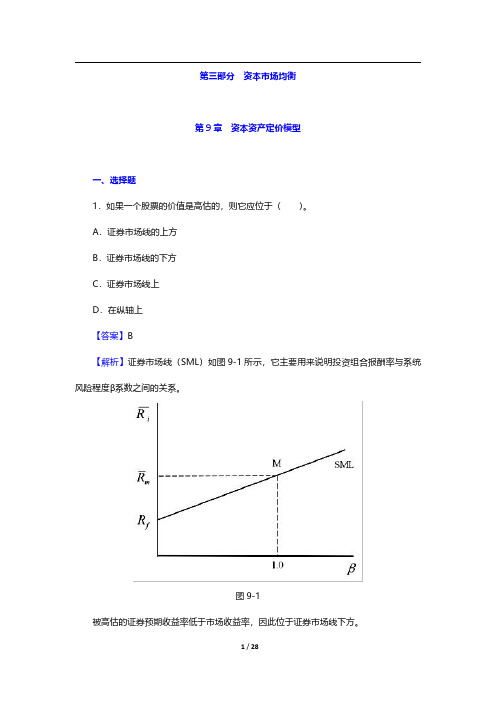
第三部分资本市场均衡第9章资本资产定价模型一、选择题1．如果一个股票的价值是高估的，则它应位于（）。

A．证券市场线的上方B．证券市场线的下方C．证券市场线上D．在纵轴上【答案】B【解析】证券市场线（SML）如图9-1所示，它主要用来说明投资组合报酬率与系统风险程度β系数之间的关系。

图9-1被高估的证券预期收益率低于市场收益率，因此位于证券市场线下方。

2．无风险利率和市场预期收益率分别是3.5%和10.5%。

根据资本资产定价模型，一只β值是1.63的证券的预期收益是（）。

A．10.12%B．14.91%C．16.56%D．18.79%【答案】B【解析】根据资本资产定价模型：E（r i）＝r f＋β[E（r M）－r f]＝3.5%＋1.63×（10.5%－3.5%）＝14.91%。

3．资本资产定价模型给出了精确预测（）的方法。

A．有效投资组合B．单一资产与风险资产组合期望收益率C．不同风险收益偏好下最优风险投资组合D．资产风险及其期望收益率之间的关系【答案】D【解析】根据资本资产定价模型，每一证券的期望收益率应等于无风险利率加上该证券由β系数测定的风险溢价。

4．假定一只股票定价合理，预期收益是15%，市场预期收益是10.5%，无风险利率是3.5%，这只股票的β值是（）。

A．1.36B．1.52C．1.64D．1.75【答案】C【解析】既然α值假定为零，证券的收益就等于CAPM设定的收益。

因此，将已知的数值代入CAPM，即15%＝[3.5%＋（10.5%－3.5%）β]，解得：β＝1.64。

5．根据CAPM模型，市场期望收益率和无风险收益率分别是0.12和0.06，β值为1.2的证券A的期望收益率是（）。

A．0.068B．0.12C．0.132D．0.142【答案】C【解析】根据资本资产定价模型，E（r i）＝r f＋[E（r M）－r f]βi＝0.06＋（0.12－0.06）×1.2＝0.132。

投资学第10版课后习题答案.docx

CHAPTER 4: MUTUAL FUNDS AND OTHER INVESTMENTCOMPANIESPROBLEM SETS1.The unit investment trust should have lower operating expenses.Because the investment trust portfolio is fixed once the trust isestablished, it does not have to pay portfolio managers toconstantly monitor and rebalance the portfolio as perceivedneeds or opportunities change. Because the portfolio is fixed, theunit investment trust also incurs virtually no trading costs.2. a. Unit investment trusts : Diversification from large-scale investing,lower transaction costs associated with large-scale trading, lowmanagement fees, predictable portfolio composition, guaranteed lowportfolio turnover rate.b.Open-end mutual funds : Diversification from large-scaleinvesting, lower transaction costs associated with large-scale trading, professional management that may be able totake advantage of buy or sell opportunities as they arise,record keeping.c.Individual stocks and bonds: No management fee; ability tocoordinate realization of capital gains or losses withinvestors ’ personal tax situation s; capability of designingportfolio to investor’s specific risk and return profile.3.Open-end funds are obligated to redeem investor's shares at netasset value and thus must keep cash or cash-equivalent securitieson hand in order to meet potential redemptions. Closed-end fundsdo not need the cash reserves because there are no redemptions forclosed-end funds. Investors in closed-end funds sell their shareswhen they wish to cash out.4.Balanced funds keep relatively stable proportions of funds investedin each asset class. They are meant as convenient instruments toprovide participation in a range of asset classes. Life-cycle fundsare balanced funds whose asset mix generally depends on the age of the investor. Aggressive life-cycle funds, with larger investments in equities, are marketed to younger investors, while conservative life-cycle funds, with larger investments in fixed-income securities, are designed for older investors. Asset allocation funds, in contrast, may vary the proportions invested in each asset class by large amounts as predictions of relative performance across classes vary. Asset allocation funds therefore engage in more aggressive market timing.5.Unlike an open-end fund, in which underlying shares are redeemedwhen the fund is redeemed, a closed-end fund trades as a security in the market. Thus, their prices may differ from the NAV.6.Advantages of an ETF over a mutual fund:ETFs are continuously traded and can be sold or purchasedon margin.There are no capital gains tax triggers when an ETF issold (shares are just sold from one investor to another).Investors buy from brokers, thus eliminating the cost ofdirect marketing to individual small investors. Thisimplies lower management fees.Disadvantages of an ETF over a mutual fund:Prices can depart from NAV (unlike an open-end fund).There is a broker fee when buying and selling (unlike ano-load fund).7.The offering price includes a 6% front-end load, or salescommission, meaning that every dollar paid results in only$ going toward purchase of shares. Therefore:Offering price =NAV$10.70 = $1Load 1 0.068.NAV = Offering price(1–Load) = $.95 = $9.Stock Value Held by FundA$ 7,000,000B12,000,000C8,000,000D15,000,000Total $42,000,000Net asset value =$42,000,000$30,000 = $4,000,00010.Value of stocks sold and replaced = $15,000,000Turnover rate =$15,000,000= , or % $42,000,00011. a.$200,000,000$3,000,000NAV$39.405,000,000b.Premium (or discount) =Pr ice NAV =$36$39.40 =–, or %NAV$39.40 The fund sells at an % discount from NAV.NAV 1 NAV 0 Distributions$12.10$12.50$1.50 12.$12.500.088, or 8.8%NAV 013. a. Start-of-year price:P0 = $×= $End-of-year price:P = $ × = $1Although NAV increased by $, the price of the fund decreased by$.Rate of return =P P Distributions$11.25$12.24$1.50100.042, or 4.2%P0$12.24b.An investor holding the same securities as the fund managerwould have earned a rate of return based on the increase inthe NAV of the portfolio:NAV 1 NAV 0 Distributions$12.10$12.00$1.50NAV 0$12.000.133, or 13.3%14. a. Empirical research indicates that past performance of mutualfunds is not highly predictive of future performance,especially for better-performing funds. While there maybe some tendency for the fund to be an above average performer nextyear, it is unlikely to once again be a top 10% performer.b.On the other hand, the evidence is more suggestive of atendency for poor performance to persist. This tendency isprobably related to fund costs and turnover rates. Thus ifthe fund is among the poorest performers, investors shouldbe concerned that the poor performance will persist.15.NAV0 = $200,000,000/10,000,000 = $20Dividends per share = $2,000,000/10,000,000 = $NAV is based on the 8% price gain, less the 1% 12b-1 fee: 1NAV1 = $20(1 – = $Rate of return =$21.384 $20$0.20 = , or %$2016.The excess of purchases over sales must be due to new inflowsinto the fund. Therefore, $400 million of stock previously held by thefund was replaced by new holdings. So turnover is: $400/$2,200 = ,or %.17. Fees paid to investment managers were: $ billion = $ million Since thetotal expense ratio was % and the management fee was %, weconclude that % must be for other expenses. Therefore, otheradministrative expenses were:$ billion = $ million.18.As an initial approximation, your return equals the return on the sharesminus the total of the expense ratio and purchase costs: 12%%4% = %.But the precise return is less than this because the 4% loadis paid up front, not at the end of the year.To purchase the shares, you would have had to invest:$20,000/(1 = $20,833.The shares increase in value from $20,000 to:= $20,000 $22,160.The rate of return is: ($22,160$20,833)/$20,833 = %.19.Assume $1,000 investment Loaded-Up Fund Economy Fund Yearly growth ( r is 6%)(1 r .01 .0075)(.98) (1 r .0025) t= 1 year$1,$1,t= 3 years$1,$1,t= 10 years$1,$1,20.a. $450,000,000 $10,000000 $1044,000,000b. The redemption of 1 million shares will most likely trigger capitalgains taxes which will lower the remaining portfolio by an amountgreater than $10,000,000 (implying a remaining total value lessthan $440,000,000). The outstanding shares fall to 43 million andthe NAV drops to below $10.21.Suppose you have $1,000 to invest. The initial investment inClass A shares is $940 net of the front-end load. After four years,your portfolio will be worth:$940 4 = $1,Class B shares allow you to invest the full $1,000, but yourinvestment performance net of 12b-1 fees will be only %, andyou will pay a 1% back-end load fee if you sell after four years.Your portfolio value after four years will be:$1,000 4 = $1,After paying the back-end load fee, your portfolio value will be:$1,.99 = $1,Class B shares are the better choice if your horizon is four years.With a 15-year horizon, the Class A shares will be worth:$94015 = $3,For the Class B shares, there is no back-end load in this casesince the horizon is greater than five years. Therefore, thevalue of the Class B shares will be:$1,00015 = $3,At this longer horizon, Class B shares are no longer the betterchoice. The effect of Class B's % 12b-1 fees accumulates over timeand finally overwhelms the 6% load charged to Class A investors.22. a.After two years, each dollar invested in a fund with a 4%load and a portfolio return equal to r will grow to: $ 2.(1 +r–Each dollar invested in the bank CD will grow to: $1.If the mutual fund is to be the better investment, thenthe portfolio return ( r ) must satisfy:(1 +r –2>(1 +r – 2 >(1 + r–2>1 + r – >1 + r >Therefore: r > = %b.If you invest for six years, then the portfolio returnmust satisfy:(1 + r –6 > =(1 +r–6>1 +r–>r > %The cutoff rate of return is lower for the six-year investment because the “fixed cost ” (the one -time front-end load) is spread over a greater number of years.c. With a 12b-1 fee instead of a front-end load, the portfoliomust earn a rate of return ( r ) that satisfies:1 + r – – >In this case, r must exceed % regardless of the investmenthorizon.23. The turnover rate is 50%. This means that, on average, 50% of theportfolio is sold and replaced with other securities each year.Trading costs on the sell orders are % and the buy orders toreplace those securities entail another % in trading costs. Totaltrading costs will reduce portfolio returns by: 2 % = %24. For the bond fund, the fraction of portfolio income given upto fees is:0.6% 4.0%= , or %For the equity fund, the fraction of investment earnings givenup to fees is:0. 6% = , or %12.0%Fees are a much higher fraction of expected earnings for thebond fund and therefore may be a more important factor inselecting the bond fund.This may help to explain why unmanaged unit investment trusts are concentrated in the fixed income market. The advantages of unitinvestment trusts are low turnover, low trading costs, and lowmanagement fees. This is a more important concern to bond-market investors.25. Suppose that finishing in the top half of all portfolio managersis purely luck, and that the probability of doing so in any year isexactly ? . Then the probability that any particular manager would5 = finish in the top half of the sample five years in a row is (?)1/32. We would then expect to find that [350 (1/32)] = 11managers finish in the top half for each of the five consecutiveyears. This is precisely what we found. Thus, we should not conclude that the consistent performance after five years is proof of skill. We would expect to find 11 managers exhibiting precisely this level of "consistency" even if performance is due solely to luck.。

投资学第10版课后习题答案

投资学第10版课后习题答案CHAPTER 7: OPTIMAL RISKY PORTFOLIOSPROBLEM SETS1. (a) and (e). Short-term rates and labor issues are factors thatare common to all firms and therefore must be considered as market risk factors. The remaining three factors are unique to this corporation and are not a part of market risk.2. (a) and (c). After real estate is added to the portfolio, there arefour asset classes in the portfolio: stocks, bonds, cash, and real estate. Portfolio variance now includes a variance term for real estate returns and a covariance term for real estate returns with returns for each of the other three asset classes. Therefore, portfolio risk is affected by the variance (or standard deviation) of real estate returns and the correlation between real estatereturns and returns for each of the other asset classes. (Note that the correlation between real estate returns and returns for cash is most likely zero.)3. (a) Answer (a) is valid because it provides the definition of theminimum variance portfolio.4. The parameters of the opportunity set are:E (r S ) = 20%, E (r B ) = 12%, σS = 30%, σB = 15%, ρ =From the standard deviations and the correlation coefficient we generate the covariance matrix [note that (,)S B S B Cov r r ρσσ=??]: Bonds Stocks Bonds 225 45 Stocks 45 900The minimum-variance portfolio is computed as follows:w Min (S ) =1739.0)452(22590045225)(Cov 2)(Cov 222=?-+-=-+-B S B S B S B ,r r ,r r σσσ w Min (B ) = 1 =The minimum variance portfolio mean and standard deviation are:E (r Min ) = × .20) + × .12) = .1339 = %σMin = 2/12222)],(Cov 2[B S B S B B S Sr r w w w w ++σσ = [ 900) + 225) + (2 45)]1/2= %5.Proportion in Stock Fund Proportionin Bond Fund ExpectedReturnStandard Deviation% % % %minimumtangencyGraph shown below.0.005.0010.0015.0020.0025.000.00 5.00 10.00 15.00 20.00 25.00 30.00Tangency PortfolioMinimum Variance PortfolioEfficient frontier of risky assetsCMLINVESTMENT OPPORTUNITY SETr f = 8.006. The above graph indicates that the optimal portfolio is thetangency portfolio with expected return approximately % andstandard deviation approximately %.7. The proportion of the optimal risky portfolio invested in the stockfund is given by:222[()][()](,)[()][()][()()](,)S f B B f S B S S f B B f SS f B f S B E r r E r r Cov r r w E r r E r r E r r E r r Cov r r σσσ-?--?=-?+-?--+-?[(.20.08)225][(.12.08)45]0.4516[(.20.08)225][(.12.08)900][(.20.08.12.08)45]-?--?==-?+-?--+-?10.45160.5484B w =-=The mean and standard deviation of the optimal risky portfolio are:E (r P ) = × .20) + × .12) = .1561 = % σp = [ 900) +225) + (2× 45)]1/2= %8. The reward-to-volatility ratio of the optimal CAL is:().1561.080.4601.1654p fpE r r σ--==9. a. If you require that your portfolio yield an expected return of14%, then you can find the corresponding standard deviation from the optimal CAL. The equation for this CAL is:()().080.4601p fC f C C PE r r E r r σσσ-=+=+If E (r C ) is equal to 14%, then the standard deviation of the portfolio is %.b. To find the proportion invested in the T-bill fund, rememberthat the mean of the complete portfolio ., 14%) is an average of the T-bill rate and the optimal combination of stocks and bonds (P ). Let y be the proportion invested in the portfolio P . The mean of any portfolio along the optimal CAL is:()(1)()[()].08(.1561.08)C f P f P f E r y r y E r r y E r r y =-?+?=+?-=+?-Setting E (r C ) = 14% we find: y = and (1 ? y ) = (the proportion invested in the T-bill fund).To find the proportions invested in each of the funds, multiply times the respective proportions of stocks and bonds in the optimal risky portfolio:Proportion of stocks in complete portfolio = =Proportion of bonds in complete portfolio = =10. Using only the stock and bond funds to achieve a portfolio expectedreturn of 14%, we must find the appropriate proportion in the stock fund (w S) and the appropriate proportion in the bond fund (w B = 1 ?w S) as follows:= × w S + × (1 ?w S) = + × w S w S =So the proportions are 25% invested in the stock fund and 75% inthe bond fund. The standard deviation of this portfolio will be:σP = [ 900) + 225) + (2 45)]1/2 = %This is considerably greater than the standard deviation of % achieved using T-bills and the optimal portfolio.11. a.Even though it seems that gold is dominated by stocks, gold mightstill be an attractive asset to hold as a part of a portfolio. If the correlation between gold and stocks is sufficiently low, goldwill be held as a component in a portfolio, specifically, the optimal tangency portfolio.b.If the correlation between gold and stocks equals +1, then no onewould hold gold. The optimal CAL would be composed of bills andstocks only. Since the set of risk/return combinations of stocksand gold would plot as a straight line with a negative slope (seethe following graph), these combinations would be dominated bythe stock portfolio. Of course, this situation could not persist.If no one desired gold, its price would fall and its expected rate of return would increase until it became sufficientlyattractive to include in a portfolio.12. Since Stock A and Stock B are perfectly negatively correlated, arisk-free portfolio can be created and the rate of return for thisportfolio, in equilibrium, will be the risk-free rate. To find the proportions of this portfolio [with the proportion w A invested inStock A and w B = (1 –w A) invested in Stock B], set the standarddeviation equal to zero. With perfect negative correlation, theportfolio standard deviation is:σP = Absolute value [w AσA w BσB]0 = 5 × w A? [10 (1 –w A)] w A =The expected rate of return for this risk-free portfolio is:E(r) = × 10) + × 15) = %Therefore, the risk-free rate is: %13. False. If the borrowing and lending rates are not identical, then,depending on the tastes of the individuals (that is, the shape oftheir indifference curves), borrowers and lenders could have different optimal risky portfolios.14. False. The portfolio standard deviation equals the weighted averageof the component-asset standard deviations only in the special case that all assets are perfectly positively correlated. Otherwise, as the formula for portfolio standard deviation shows, the portfoliostandard deviation is less than the weighted average of the component-asset standard deviations. The portfolio variance is aweighted sum of the elements in the covariance matrix, with theproducts of the portfolio proportions as weights.15. The probability distribution is:Probability Rate ofReturn100%50Mean = [ × 100%] + [ × (-50%)] = 55%Variance = [ × (100 ? 55)2] + [ × (-50 ? 55)2] = 4725Standard deviation = 47251/2 = %16. σP = 30 = y× σ = 40 × y y =E(r P) = 12 + (30 ? 12) = %17. The correct choice is (c). Intuitively, we note that since allstocks have the same expected rate of return and standard deviation, we choose the stock that will result in lowest risk. This is thestock that has the lowest correlation with Stock A.More formally, we note that when all stocks have the same expected rate of return, the optimal portfolio for any risk-averse investor is the global minimum variance portfolio (G). When the portfolio is restricted to Stock A and one additional stock, the objective is to find G for any pair that includes Stock A, and then select thecombination with the lowest variance. With two stocks, I and J, theformula for the weights in G is:)(1)(),(Cov 2),(Cov )(222I w J w r r r r I w Min Min J I J I J I J Min -=-+-=σσσSince all standard deviations are equal to 20%:(,)400and ()()0.5I J I J Min Min Cov r r w I w J ρσσρ====This intuitive result is an implication of a property of any efficient frontier, namely, that the covariances of the global minimum variance portfolio with all other assets on the frontier are identical and equal to its own variance. (Otherwise, additional diversification would further reduce the variance.) In this case, the standard deviation of G(I, J) reduces to:1/2()[200(1)]Min IJ G σρ=?+This leads to the intuitive result that the desired addition would be the stock with the lowest correlation with Stock A, which is Stock D. The optimal portfolio is equally invested in StockA and Stock D, and the standard deviation is %.18. No, the answer to Problem 17 would not change, at least as long asinvestors are not risk lovers. Risk neutral investors would not care which portfolio they held since all portfolios have an expected return of 8%.19. Yes, the answers to Problems 17 and 18 would change. The efficientfrontier of risky assets is horizontal at 8%, so the optimal CAL runs from the risk-free rate through G. This implies risk-averse investors will just hold Treasury bills.20. Rearrange the table (converting rows to columns) and compute serialcorrelation results in the following table:Nominal RatesFor example: to compute serial correlation in decade nominalreturns for large-company stocks, we set up the following twocolumns in an Excel spreadsheet. Then, use the Excel function“CORREL” to calculate the correlation for the data.Decade Previous1930s%%1940s%%1950s%%1960s%%1970s%%1980s%%1990s%%Note that each correlation is based on only seven observations, so we cannot arrive at any statistically significant conclusions.Looking at the results, however, it appears that, with theexception of large-company stocks, there is persistent serial correlation. (This conclusion changes when we turn to real rates in the next problem.)21. The table for real rates (using the approximation of subtracting adecade’s average inflation from the decade’s average nominalreturn) is:Real RatesSmall Company StocksLarge Company StocksLong-TermGovernmentBondsIntermed-TermGovernmentBondsTreasuryBills 1920s1930s1940s1950s1960s1970s1980s1990sSerialCorrelationWhile the serial correlation in decade nominal returns seems to be positive, it appears that real rates are serially uncorrelated. The decade time series (although again too short for any definitiveconclusions) suggest that real rates of return are independent from decade to decade.22. The 3-year risk premium for the S&P portfolio is, the 3-year risk premium for thehedge fund portfolio is S&P 3-year standard deviation is 0. The hedge fund 3-year standard deviation is 0. S&P Sharpe ratio is = , and the hedge fund Sharpe ratio is = .23. With a ρ = 0, the optimal asset allocation is,.With these weights,EThe resulting Sharpe ratio is = . Greta has a risk aversion of A=3, Therefore, she will investyof her wealth in this risky portfolio. The resulting investment composition will be S&P: = % and Hedge: = %. The remaining 26% will be invested in the risk-free asset.24. With ρ = , the annual covariance is .25. S&P 3-year standard deviation is . The hedge fund 3-year standard deviation is . Therefore, the 3-year covariance is 0.26. With a ρ=.3, the optimal asset allocation is, .With these weights,E. The resulting Sharpe ratio is = . Notice that the higher covariance results in a poorer Sharpe ratio.Greta will investyof her wealth in this risky portfolio. The resulting investment composition will be S&P: =% and hedge: = %. The remaining % will be invested in the risk-free asset.CFA PROBLEMS1. a. Restricting the portfolio to 20 stocks, rather than 40 to 50stocks, will increase the risk of the portfolio, but it ispossible that the increase in risk will be minimal. Suppose that, for instance, the 50 stocks in a universe have the samestandard deviation () and the correlations between each pair are identical, with correlation coefficient ρ. Then, the covariance between each pair of stocks would be ρσ2, and the variance of an equally weighted portfolio would be:222ρσ1σ1σnn n P -+=The effect of the reduction in n on the second term on the right-hand side would be relatively small (since 49/50 is close to 19/20 and ρσ2 is smaller than σ2), but thedenominator of the first term would be 20 instead of 50. For example, if σ = 45% and ρ = , then the standard deviation with 50 stocks would be %, and would rise to % when only 20 stocks are held. Such an increase might be acceptable if the expected return is increased sufficiently.b. Hennessy could contain the increase in risk by making sure thathe maintains reasonable diversification among the 20 stocks that remain in his portfolio. This entails maintaining a low correlation among the remaining stocks. For example, in part (a), with ρ = , the increase in portfolio risk was minimal. As a practical matter, this means that Hennessy would have to spread his portfolio among many industries; concentrating on just a few industries would result in higher correlations among the included stocks.2. Risk reduction benefits from diversification are not a linearfunction of the number of issues in the portfolio. Rather, the incremental benefits from additional diversification are most important when you are least diversified. Restricting Hennessy to 10 instead of 20 issues would increase the risk of hisportfolio by a greater amount than would a reduction in the size of theportfolio from 30 to 20 stocks. In our example, restricting the number of stocks to 10 will increase the standard deviation to %. The % increase in standard deviation resulting from giving up 10 of20 stocks is greater than the % increase that results from givingup 30 of 50 stocks.3. The point is well taken because the committee should be concernedwith the volatility of the entire portfolio. Since Hennessy’s portfolio is only one of six well-diversified portfolios and is smaller than the average, the concentration in fewer issues mighthave a minimal effect on the diversification of the total fund.Hence, unleashing Hennessy to do stock picking may be advantageous.4. d. Portfolio Y cannot be efficient because it is dominated byanother portfolio. For example, Portfolio X has both higher expected return and lower standard deviation.5. c.6. d.7. b.8. a.9. c.10. Since we do not have any information about expected returns, wefocus exclusively on reducing variability. Stocks A and C haveequal standard deviations, but the correlation of Stock B with Stock C is less than that of Stock A with Stock B . Therefore, a portfoliocomposed of Stocks B and C will have lower total risk than a portfolio composed of Stocks A and B.11. Fund D represents the single best addition to complementStephenson's current portfolio, given his selection criteria. Fund D’s expected return percent) has the potential to increase theportfolio’s return somewhat. Fund D’s relatively low correlation with his current portfolio (+ indicates that Fund D will providegreater diversification benefits than any of the other alternativesexcept Fund B. The result of adding Fund D should be a portfolio with approximately the same expected return and somewhat lower volatility compared to the original portfolio.The other three funds have shortcomings in terms of expected return enhancement or volatility reduction through diversification. Fund A offers the potential for increasing the portfolio’s return but is too highly correlated to provide substantial volatility reduction benefits through diversification. Fund B provides substantial volatility reduction through diversification benefits but is expected to generate a return well below the current portfolio’s return. Fund C has the greatest potential to increase th e portfolio’s return but is too highly correlated with the current portfolio to provide substantial volatility reduction benefits through diversification.12. a. Subscript OP refers to the original portfolio, ABC to thenew stock, and NP to the new portfolio.i. E(r NP) = w OP E(r OP) + w ABC E(r ABC) = + = %ii. Cov = ρOP ABC = =iii. NP = [w OP2OP2 + w ABC2ABC2 + 2 w OP w ABC(Cov OP , ABC)]1/2= [ 2 + + (2 ]1/2= % %b. Subscript OP refers to the original portfolio, GS to governmentsecurities, and NP to the new portfolio.i. E(r NP) = w OP E(r OP) + w GS E(r GS) = + = %ii. Cov = ρOP GS = 0 0 = 0iii. NP = [w OP2OP2 + w GS2GS2 + 2 w OP w GS (Cov OP , GS)]1/2= [ + 0) + (2 0)]1/2= % %c. Adding the risk-free government securities would result in alower beta for the new portfolio. The new portfolio beta will bea weighted average of the individual security betas in theportfolio; the presence of the risk-free securities would lower that weighted average.d. The comment is not correct. Although the respective standarddeviations and expected returns for the two securities under consideration are equal, the covariances between each security andthe original portfolio are unknown, making it impossible to drawthe conclusion stated. For instance, if the covariances aredifferent, selecting one security over the other may result in alower standard deviation for the portfolio as a whole. In such acase, that security would be the preferred investment, assumingall other factors are equal.e. i. Grace clearly expressed the sentiment that the risk of losswas more important to her than the opportunity for return. Usingvariance (or standard deviation) as a measure of risk in her casehas a serious limitation because standard deviation does not distinguish between positive and negative price movements.ii. Two alternative risk measures that could be used instead ofvariance are:Range of returns, which considers the highest and lowestexpected returns in the future period, with a larger rangebeing a sign of greater variability and therefore of greaterrisk.Semivariance can be used to measure expected deviations of returns below the mean, or some other benchmark, such as zero.Either of these measures would potentially be superior tovariance for Grace. Range of returns would help to highlight the full spectrum of risk she is assuming, especially thedownside portion of the range about which she is so concerned.Semivariance would also be effective, because it implicitlyassumes that the investor wants to minimize the likelihood ofreturns falling below some target rate; in Grace’s case, the target rate would be set at zero (to protect against negative returns).13. a. Systematic risk refers to fluctuations in asset prices causedby macroeconomic factors that are common to all risky assets;hence systematic risk is often referred to as market risk.Examples of systematic risk factors include the business cycle, inflation, monetary policy, fiscal policy, and technologicalchanges.Firm-specific risk refers to fluctuations in asset pricescaused by factors that are independent of the market, such asindustry characteristics or firm characteristics. Examples offirm-specific risk factors include litigation, patents,management, operating cash flow changes, and financial leverage.b. Trudy should explain to the client that picking only the topfive best ideas would most likely result in the client holdinga much more risky portfolio. The total risk of a portfolio, orportfolio variance, is the combination of systematic risk and firm-specific risk.The systematic component depends on the sensitivity of the individual assets to market movements as measured by beta.Assuming the portfolio is well diversified, the number ofassets will not affect the systematic risk component ofportfolio variance. The portfolio beta depends on theindividual security betas and the portfolio weights of those securities.On the other hand, the components of firm-specific risk (sometimes called nonsystematic risk) are not perfectly positively correlated with each other and, as more assets are added to the portfolio, those additional assets tend to reduce portfolio risk. Hence, increasing the number of securities in a portfolio reduces firm-specific risk. For example, a patent expiration for one company would not affect the othersecurities in the portfolio. An increase in oil prices islikely to cause a drop in the price of an airline stock butwill likely result in an increase in the price of an energy stock. As the number of randomly selected securities increases, the total risk (variance) of the portfolio approaches its systematic variance.。

投资学第10版课后习题答案

CHAPTER 4: MUTUAL FUNDS AND OTHER INVESTMENTCOMPANIESPROBLEM SETS1. The unit investment trust should have lower operating expenses.Because the investment trust portfolio is fixed once the trust isestablished, it does not have to pay portfolio managers toconstantly monitor and rebalance the portfolio as perceived needsor opportunities change. Because the portfolio is fixed, the unitinvestment trust also incurs virtually no trading costs.2. a. Unit investment trusts: Diversification from large-scaleinvesting, lower transaction costs associated with large-scaletrading, low management fees, predictable portfolio composition,guaranteed low portfolio turnover rate.b. Open-end mutual funds: Diversification from large-scaleinvesting, lower transaction costs associated with large-scaletrading, professional management that may be able to takeadvantage of buy or sell opportunities as they arise, recordkeeping.c. Individual stocks and bonds: No management fee; ability tocoordinate realization of capital gains or losses withinvestors’ personal tax situation s; capability of designingportfolio to investor’s specific risk and return profile.3. Open-end funds are obligated to redeem investor's shares at netasset value and thus must keep cash or cash-equivalent securitieson hand in order to meet potential redemptions. Closed-end funds do not need the cash reserves because there are no redemptions forclosed-end funds. Investors in closed-end funds sell their shareswhen they wish to cash out.4. Balanced funds keep relatively stable proportions of funds investedin each asset class. They are meant as convenient instruments toprovide participation in a range of asset classes. Life-cycle fundsare balanced funds whose asset mix generally depends on the age of the investor. Aggressive life-cycle funds, with larger investments in equities, are marketed to younger investors, while conservative life-cycle funds, with larger investments in fixed-income securities, are designed for older investors. Asset allocation funds, in contrast, may vary the proportions invested in each asset class by large amounts as predictions of relative performance across classes vary. Asset allocation funds therefore engage in more aggressive market timing.5. Unlike an open-end fund, in which underlying shares are redeemedwhen the fund is redeemed, a closed-end fund trades as a security in the market. Thus, their prices may differ from the NAV.6. Advantages of an ETF over a mutual fund:ETFs are continuously traded and can be sold or purchased on margin.There are no capital gains tax triggers when an ETF is sold(shares are just sold from one investor to another).Investors buy from brokers, thus eliminating the cost ofdirect marketing to individual small investors. This implieslower management fees.Disadvantages of an ETF over a mutual fund:Prices can depart from NAV (unlike an open-end fund).There is a broker fee when buying and selling (unlike a no-load fund).7. The offering price includes a 6% front-end load, or salescommission, meaning that every dollar paid results in only $ going toward purchase of shares. Therefore: Offering price =06.0170.10$Load 1NAV -=-= $8. NAV = Offering price (1 –Load) = $ .95 = $9. Stock Value Held by FundA $ 7,000,000B 12,000,000C 8,000,000D 15,000,000Total $42,000,000Net asset value =000,000,4000,30$000,000,42$-= $10. Value of stocks sold and replaced = $15,000,000 Turnover rate =000,000,42$000,000,15$= , or %11. a. 40.39$000,000,5000,000,3$000,000,200$NAV =-=b. Premium (or discount) = NAVNAV ice Pr - = 40.39$40.39$36$-= –, or % The fund sells at an % discount from NAV.12. 100NAV NAV Distributions $12.10$12.50$1.500.088, or 8.8%NAV $12.50-+-+==13. a. Start-of-year price: P 0 = $ × = $End-of-year price: P 1 = $ × = $Although NAV increased by $, the price of the fund decreased by $. Rate of return =100Distributions $11.25$12.24$1.500.042, or 4.2%$12.24P P P -+-+==b. An investor holding the same securities as the fund managerwould have earned a rate of return based on the increase in the NAV of the portfolio:100NAV NAV Distributions $12.10$12.00$1.500.133, or 13.3%NAV $12.00-+-+==14. a. Empirical research indicates that past performance of mutualfunds is not highly predictive of future performance,especially for better-performing funds. While there may be some tendency for the fund to be an above average performer nextyear, it is unlikely to once again be a top 10% performer.b. On the other hand, the evidence is more suggestive of atendency for poor performance to persist. This tendency isprobably related to fund costs and turnover rates. Thus if the fund is among the poorest performers, investors should beconcerned that the poor performance will persist.15. NAV 0 = $200,000,000/10,000,000 = $20Dividends per share = $2,000,000/10,000,000 = $NAV1 is based on the 8% price gain, less the 1% 12b-1 fee: NAV1 = $20 (1 – = $Rate of return =20$20 .0$20$384.21$+-= , or %16. The excess of purchases over sales must be due to new inflows intothe fund. Therefore, $400 million of stock previously held by the fund was replaced by new holdings. So turnover is: $400/$2,200 = , or %.17. Fees paid to investment managers were: $ billion = $ millionSince the total expense ratio was % and the management fee was %, we conclude that % must be for other expenses. Therefore, other administrative expenses were: $ billion = $ million.18. As an initial approximation, your return equals the return on the shares minus the total of the expense ratio and purchase costs: 12% % 4% = %.But the precise return is less than this because the 4% load is paid up front, not at the end of the year. To purchase the shares, you would have had to invest: $20,000/(1 = $20,833. The shares increase in value from $20,000 to: $20,000 = $22,160. The rate of return is: ($22,160 $20,833)/$20,833 = %.19. Assume $1,000 investmentLoaded-Up Fund Economy Fund Yearly growth (r is 6%) (1.01.0075)r +-- (.98)(1.0025)r ⨯+- t = 1 year$1, $1, t = 3 years$1, $1, t = 10 years$1, $1,20. a. $450,000,000$10,000000$1044,000,000-= b. The redemption of 1 million shares will most likely triggercapital gains taxes which will lower the remaining portfolio by an amount greater than $10,000,000 (implying a remaining total value less than $440,000,000). The outstanding shares fall to 43 million and the NAV drops to below $10.21. Suppose you have $1,000 to invest. The initial investment in ClassA shares is $940 net of the front-end load. After four years, yourportfolio will be worth:$940 4 = $1,Class B shares allow you to invest the full $1,000, but yourinvestment performance net of 12b-1 fees will be only %, and you will pay a 1% back-end load fee if you sell after four years. Your portfolio value after four years will be:$1,000 4 = $1,After paying the back-end load fee, your portfolio value will be:$1, .99 = $1,Class B shares are the better choice if your horizon is four years.With a 15-year horizon, the Class A shares will be worth:$940 15 = $3,For the Class B shares, there is no back-end load in this casesince the horizon is greater than five years. Therefore, the value of the Class B shares will be:$1,000 15 = $3,At this longer horizon, Class B shares are no longer the betterchoice. The effect of Class B's % 12b-1 fees accumulates over time and finally overwhelms the 6% load charged to Class A investors.22. a. After two years, each dollar invested in a fund with a 4% loadand a portfolio return equal to r will grow to: $ (1 + r–2.Each dollar invested in the bank CD will grow to: $1 .If the mutual fund is to be the better investment, then theportfolio return (r) must satisfy:(1 + r–2 >(1 + r–2 >(1 + r–2 >1 + r– >1 + r >Therefore: r > = %b. If you invest for six years, then the portfolio return mustsatisfy:(1 + r–6 > =(1 + r–6 >1 + r– >r > %The cutoff rate of return is lower for the six-year investment because the “fixed cost” (the one-time front-end load) is spread over a greater number of years.c. With a 12b-1 fee instead of a front-end load, the portfoliomust earn a rate of return (r ) that satisfies:1 + r – – >In this case, r must exceed % regardless of the investmenthorizon.23. The turnover rate is 50%. This means that, on average, 50% of theportfolio is sold and replaced with other securities each year. Trading costs on the sell orders are % and the buy orders toreplace those securities entail another % in trading costs. Total trading costs will reduce portfolio returns by: 2 % = %24. For the bond fund, the fraction of portfolio income given up tofees is: %0.4%6.0= , or % For the equity fund, the fraction of investment earnings given up to fees is:%0.12%6.0= , or % Fees are a much higher fraction of expected earnings for the bond fund and therefore may be a more important factor in selecting the bond fund.This may help to explain why unmanaged unit investment trusts are concentrated in the fixed income market. The advantages of unit investment trusts are low turnover, low trading costs, and low management fees. This is a more important concern to bond-market investors.25. Suppose that finishing in the top half of all portfolio managers ispurely luck, and that the probability of doing so in any year is exactly ½. Then the probability that any particular manager would finish in the top half of the sample five years in a row is (½)5 = 1/32. We would then expect to find that [350 (1/32)] = 11managers finish in the top half for each of the five consecutiveyears. This is precisely what we found. Thus, we should not conclude that the consistent performance after five years is proof of skill. We would expect to find 11 managers exhibiting precisely this level of "consistency" even if performance is due solely to luck.。

1、下载文档前请自行甄别文档内容的完整性，平台不提供额外的编辑、内容补充、找答案等附加服务。
2、"仅部分预览"的文档,不可在线预览部分如存在完整性等问题,可反馈申请退款(可完整预览的文档不适用该条件!)。
3、如文档侵犯您的权益，请联系客服反馈,我们会尽快为您处理(人工客服工作时间：9:00-18:30)。

CHAPTER 18: EQUITY VALUATION MODELS PROBLEM SETS1. Theoretically, dividend discount models can be used to value thestock of rapidly growing companies that do not currently paydividends; in this scenario, we would be valuing expecteddividends in the relatively more distant future. However, as apractical matter, such estimates of payments to be made in themore distant future are notoriously inaccurate, renderingdividend discount models problematic for valuation of suchcompanies; free cash flow models are more likely to beappropriate. At the other extreme, one would be more likely tochoose a dividend discount model to value a mature firm paying a relatively stable dividend.2. It is most important to use multistage dividend discount modelswhen valuing companies with temporarily high growth rates. These companies tend to be companies in the early phases of their life cycles, when they have numerous opportunities for reinvestment, resulting in relatively rapid growth and relatively low dividends (or, in many cases, no dividends at all). As these firms mature, attractive investment opportunities are less numerous so thatgrowth rates slow.3. The intrinsic value of a share of stock is the individualinvestor’s assessment of the true worth of the stock. The market capitalization rate is the market consensus for the required rate of return for the stock. If the intrinsic value of the stock is equal to its price, then the market capitalization rate is equal to the expected rate of return. On the other hand, if the individual investor believes the stock is underpriced ., intrinsic value > price), then that investor’s expected rate of return is greater than the market capitalization rate.4. First estimate the amount of each of the next two dividends andthe terminal value. The current value is the sum of the present value of these cash flows, discounted at %.5. The required return is 9%. $1.22(1.05)0.05.09,or 9%$32.03k ⨯=+=6. The Gordon DDM uses the dividend for period (t +1) which would be .$1.05$35(0.05)$1.050.050.088%$35k k =-=+==7. The PVGO is $: $3.64$41$0.560.09PVGO =-=1$20.160.12,or 12%$50D k g P g g =+=+⇒=8. a.b. 10$2$18.180.160.05D P k g ===-- The price falls in response to the more pessimistic dividend forecast. The forecast for current year earnings, however, is unchanged. Therefore, the P/E ratio falls. The lower P/E ratio is evidence of the diminished optimism concerning the firm's growth prospects.9. a. g = ROEb = 16%= 8%D 1 = $2 (1 – b ) = $2 (1 – = $110$1$25.000.120.08D P k g ===--b. P 3 = P 0(1 + g )3 = $253 = $10. a.b. Leading P 0/E 1 = $$ =1010[()]6% 1.25(14%6%)16%29%6%31(1)(1)$3(1.06)$1.063$1.06$10.600.160.06f m f k r E r rg D E g b D P k g β=+⨯-=+⨯-==⨯==⨯+⨯-=⨯⨯====--Trailing P 0/E 0 = $$ =c. 10$3.18$10.60$9.2750.16E PVGO P k =-=-=- The low P/E ratios and negative PVGO are due to a poor ROE (9%) that is less than the market capitalization rate (16%).d. Now, you revise b to 1/3, g to 1/39% = 3%, and D 1 to:E 0 (1 + g ) (2/3)$3(2/3) = $Thus:V 0 = $ – = $V 0 increases because the firm pays out more earnings instead of reinvesting a poor ROE. This information is not yet known to the rest of the market.11. a. 10$8$1600.100.05D P k g ===--b. The dividend payout ratio is 8/12 = 2/3, so the plowbackratio is b = 1/3. The implied value of ROE on future investments is found by solving:g = bROE with g = 5% and b = 1/3 ROE = 15%c. Assuming ROE = k , price is equal to:10$12$1200.10E P k ===Therefore, the market is paying $40 per share ($160 – $120) for growth opportunities.12. a. k = D 1/P 0 + gD 1 = $2 = $1 g = b ROE = =Therefore: k = ($1/$10) + = , or 20%b. Since k = ROE, the NPV of future investment opportunities iszero:10$10$100E PVGO P k=-=-= c. Since k = ROE, the stock price would be unaffected bycutting the dividend and investing the additional earnings.13. a. k = r f + β [E (r M ) – r f ] = 8% + (15% – 8%) = %g = b ROE =20% = 12%00(1)$4 1.12$101.820.1640.12D g V k g +⨯===--b. P 1 = V 1 = V 0(1 + g ) = $= $1100$4.48$114.04$100()0.1852,or 18.52%$100D P PE r P -++-===14.Time:0 1 5 6 E t$$$$D t $$$$ b g%%%%The year-6 earnings estimate is based on growth rate of × = .a. 65$10.85$180.820.150.09D V k g ===⇒-- 5055$180.82$89.90(1) 1.15V V k ===+b. The price should rise by 15% per year until year 6: becausethere is no dividend, the entire return must be in capital gains.c. The payout ratio would have no effect on intrinsic valuebecause ROE = k .15. a. The solution is shown in the Excel spreadsheet below:values are $ and $, respectively.16. The solutions derived from Spreadsheet are as follows:Intrinsic Value:FCFF IntrinsicValue:FCFEIntrinsicValue perShare: FCFFIntrinsicValue perShare: FCFEa.100,00075,128b.109,42281,795c.89,69366,01417.Time:0123D t $ $ $ $ g % % % %a. The dividend to be paid at the end of year 3 is the firstinstallment of a dividend stream that will increaseindefinitely at the constant growth rate of 5%. Therefore, we can use the constant growth model as of the end of year 2 in order to calculate intrinsic value by adding the present value of the first two dividends plus the present value of the price of the stock at the end of year 2. The expected price 2 years from now is:P 2 = D 3/(k – g ) = $ – = $ The PV of this expected price is $ = $The PV of expected dividends in years 1 and 2 is13.2$20.15625.1$20.125.1$2=+ Thus the current price should be: $ + $ = $b. Expected dividend yield = D 1/P 0 = $$ = , or %c. The expected price one year from now is the PV at that timeof P 2 and D 2:P 1 = (D 2 + P 2)/ = ($ + $/ = $ The implied capital gain is(P 1 – P 0)/P 0 = ($ – $/$ = = %The sum of the implied capital gains yield and the expected dividend yield is equal to the market capitalization rate. This is consistent with the DDM.18.Time:0 1 4 5 E t $ $ $ $ D t$$$$Dividends = 0 for the next four years, so b = (100% plowback ratio). a. 54$10.368$69.120.15D P k === (Since k =ROE, knowing the plowback rate is unnecessary)4044$69.12$39.52(1) 1.15P V k ===+b. Price should increase at a rate of 15% over the next year,so that the HPR will equal k .19. Before-tax cash flow from operations$2,100,000 Depreciation 210,000 Taxable Income 1,890,000 Taxes (@ 35%)661,500 After-tax unleveraged income 1,228,500After-tax cash flow from operations(After-tax unleveraged income + depreciation) 1,438,500New investment (20% of cash flow from operations) 420,000Free cash flow(After-tax cash flow from operations – new investment)$1,018,500The value of the firm ., debt plus equity) is:000,550,14$05.012.0500,018,1$10=-=-=g k C V Since the value of the debt is $4 million, the value of the equity is $10,550,000.20. a. g = ROEb = 20% = 10%010(1)$0.50 1.10$110.150.10D g D P k g k g +⨯====---b.Time EPS Dividen dComment0 $ $1 g = 10%, plowback =2EPS has grown by 10% based on last year’s earnings plowback and ROE; this year’s earnings plowback ratio now falls to and payout ratio =3 $ $ EPS grows by (15%) = 6% and payout ratio =At time 2: 32$0.7696$8.5510.150.06D P k g ===-- At time 0: 02$0.55$0.726$8.551$7.4931.15(1.15)V +=+=c. P 0 = $11 and P 1 = P 0(1 + g ) = $(Because the market is unaware of the changed competitivesituation, it believes the stock price should grow at 10% per year.)P 2 = $ after the market becomes aware of the changed competitive situation.P 3 = $ = $ (The new growth rate is 6%.)YearReturn 1($12.10$11)$0.550.150,or 15.0%$11-+= 2($8.551$12.10)$0.7260.233,or 23.3%$12.10-+=-- 3 ($9.064$8.551)$0.76960.150,or 15.0%$8.551-+= Moral: In normal periods when there is no special information, the stock return = k = 15%. When special information arrives, all the abnormal return accrues in that period , as one would expect in an efficient market.CFA PROBLEMS1. a. This director is confused. In the context of the constant growth model[., P 0 = D 1/ k – g )], it is true that price is higher whendividends are higher holding everything else includingdividend growth constant . But everything else will not beconstant. If the firm increases the dividend payout rate, the growth rate g will fall, and stock price will not necessarily rise. In fact, if ROE > k , price will fall.b. (i) An increase in dividend payout will reduce thesustainable growth rate as less funds are reinvested in thefirm. The sustainable growth rate . ROE plowback) will fall as plowback ratio falls.(ii) The increased dividend payout rate will reduce thegrowth rate of book value for the same reason -- less fundsare reinvested in the firm.2. Using a two-stage dividend discount model, the current value of ashare of Sundanci is calculated as follows.3120122()(1)(1)(1)D D D k g V k k k -=+++++ 98.43$14.1)13.014.0(5623.0$14.14976.0$14.13770.0$221=-++= where:E0 = $D0 = $E1 = E01 = $ = $D1 = E1 = $ = $E2 = E02 = $ 2 = $D2 = E2 = $ = $E3 = E02 = $ 2 = $ D3 = E3 = $ = $3. a. Free cash flow to equity (FCFE) is defined as the cash flowremaining after meeting all financial obligations (includingdebt payment) and after covering capital expenditure andworking capital needs. The FCFE is a measure of how much thefirm can afford to pay out as dividends but, in a given year,may be more or less than the amount actually paid out.Sundanci's FCFE for the year 2008 is computed as follows: FCFE = Earnings + Depreciation Capital expendituresIncrease in NWC= $80 million + $23 million $38 million $41 million = $24 millionFCFE per share =$24 million$0.286 # of shares outstanding84 million sharesFCFE==At this payout ratio, Sundanci's FCFE per share equalsdividends per share.b. The FCFE model requires forecasts of FCFE for the highgrowth years (2012 and 2013) plus a forecast for the first year of stable growth (2014) in order to allow for anestimate of the terminal value in 2013 based on perpetualgrowth. Because all of the components of FCFE are expected to grow at the same rate, the values can be obtained byprojecting the FCFE at the common rate. (Alternatively, the components of FCFE can be projected and aggregated for each year.)This table shows the process for estimating the current pershare value:FCFE Base AssumptionsShares outstanding: 84 million, k =14%Actual 2011Projected2012Projected2013Projected2014Growth rate (g)27%27%13%Total Per ShareEarnings after tax$80$$$$ Plus: Depreciation expense23$ Less: Capital expenditures38$ Less: Increase in net workingcapital41$ Equals: FCFE24$ Terminal value$*Total cash flows to equity$$†Discounted value$‡ $‡Current value per share$§*Projected 2013 terminal value = (Projected 2014 FCFE)/(r g)†Projected 2013 Total cash flows to equity =Projected 2013 FCFE + Projected 2013 terminal value‡Discounted values obtained using k= 14%§Current value per share=Sum of discounted projected 2012 and 2013 total FCFEc. i. The DDM uses a strict definition of cash flows to equity, .the expected dividends on the common stock. In fact, taken toits extreme, the DDM cannot be used to estimate the value of astock that pays no dividends. The FCFE model expands thedefinition of cash flows to include the balance of residual cash flows after all financial obligations and investment needs have been met. Thus the FCFE model explicitly recognizes the firm’s investment and financing policies as well as its dividend policy.In instances of a change of corporate control, and therefore the possibility of changing dividend policy, the FCFE model providesa better estimate of value. The DDM is biased toward finding lowP/E ratio stocks with high dividend yields to be undervalued and conversely, high P/E ratio stocks with low dividend yields to be overvalued. It is considered a conservative model in that ittends to identify fewer undervalued firms as market prices rise relative to fundamentals. The DDM does not allow for thepotential tax disadvantage of high dividends relative to thecapital gains achievable from retention of earnings.ii. Both two-stage valuation models allow for two distinctphases of growth, an initial finite period where the growth rate is abnormal, followed by a stable growth period that is expected to last indefinitely. These two-stage models share the samelimitations with respect to the growth assumptions. First, there is the difficulty of defining the duration of the extraordinarygrowth period. For example, a longer period of high growth willlead to a higher valuation, and there is the temptation toassume an unrealistically long period of extraordinary growth.Second, the assumption of a sudden shift from high growth tolower, stable growth is unrealistic. The transformation is morelikely to occur gradually, over a period of time. Given that theassumed total horizon does not shift ., is infinite), the timingof the shift from high to stable growth is a criticaldeterminant of the valuation estimate. Third, because the valueis quite sensitive to the steady-state growth assumption, over-or underestimating this rate can lead to large errors in value.The two models share other limitations as well, notablydifficulties in accurately forecasting required rates of return,in dealing with the distortions that result from substantialand/or volatile debt ratios, and in accurately valuing assetsthat do not generate any cash flows.4. a. The formula for calculating a price earnings ratio (P/E) fora stable growth firm is the dividend payout ratio divided bythe difference between the required rate of return and thegrowth rate of dividends. If the P/E is calculated based ontrailing earnings (year 0), the payout ratio is increased bythe growth rate. If the P/E is calculated based on nextyear’s earnings (year 1), the numerator is the payout ratio.P/E on trailing earnings:P/E = [payout ratio (1 + g)]/(k g) = [ ]/ = P/E on next year's earnings:P/E = payout ratio/(k g) = =b. The P/E ratio is a decreasing function of riskiness; as risk increases, the P/E ratio decreases. Increases in the riskiness of Sundanci stock would be expected to lower the P/E ratio. The P/E ratio is an increasing function of the growth rate of the firm; the higher the expected growth, the higher the P/E ratio. Sundanci would command a higher P/E if analysts increase the expected growth rate. The P/E ratio is a decreasing function of the market risk premium. An increased market risk premium increases the required rate of return, lowering the price of a stock relative to its earnings. A higher market risk premium would be expected to lower Sundanci's P/E ratio.5. a. The sustainable growth rate is equal to:P lowback ratio × Return on equity = b × ROENet income - (Dividends per share Shares outstanding)where Net income b ⨯=ROE = Net income/Beginning of year equityIn 2010:b = [208 – × 100)]/208 =ROE = 208/1380 =Sustainable growth rate = × = %In 2013:b = [275 – × 100)]/275 =ROE = 275/1836 =Sustainable growth rate = × = %b. i. The increased retention ratio increased the sustainablegrowth rate.Retention ratio = [Net income - (Dividend per share Shares outstanding)]Net incomeRetention ratio increased from in 2010 to in 2013.This increase in the retention ratio directly increased the sustainable growth rate because the retention ratio is one ofthe two factors determining the sustainable growth rate.ii. The decrease in leverage reduced the sustainable growth rate.Financial leverage = (Total assets/Beginning of year equity) Financial leverage decreased from (3230/1380) at the beginning of 2010 to at the beginning of 2013 (3856/1836)This decrease in leverage directly decreased ROE (and thus the sustainable growth rate) because financial leverage is one of the factors determining ROE (and ROE is one of the two factors determining the sustainable growth rate).6. a. The formula for the Gordon model is 00(1)D g V k g⨯+=- where:D 0 = Dividend paid at time of valuationg = Annual growth rate of dividendsk = Required rate of return for equityIn the above formula, P 0, the market price of the commonstock, substitutes for V 0 and g becomes the dividend growthrate implied by the market:P 0 = [D 0 × (1 + g )]/(k – g )Substituting, we have:= [ × (1 + g )]/ – g ) g = %b. Use of the Gordon growth model would be inappropriate tovalue Dynamic’s common stock, for the following reasons:i. The Gordon growth model assumes a set of relationshipsabout the growth rate for dividends, earnings, and stockvalues. Specifically, the model assumes that dividends,earnings, and stock values will grow at the same constant rate.In valuing Dynamic’s common stock, the Gordon growth model isinappropriate because management’s dividend policy has helddividends constant in dollar amount although earnings havegrown, thus reducing the payout ratio. This policy isinconsistent with the Gordon model assumption that the payout ratio is constant. ii. It could also be argued that use of the Gordon model, given Dynamic’s current dividend policy, violates one of the general conditions for suitability of the model, namely that the company’s dividend policy bears an understandable and consistent relationship with the company’s profitability.7. a.The industry’s estimated P/E can be computed using the following model: 01Payout ratio P E k g =- However, since k and g are not explicitly given, they must be computed using the following formulas: g ind = ROE Retention rate = = k ind = Government bond yield + ( Industry beta Equity risk premium) = + = Therefore: 010.6030.00.120.10P E ==-b. i. Forecast growth in real GDP would cause P/E ratios to begenerally higher for Country A. Higher expected growth inGDP implies higher earnings growth and a higher P/E.ii. Government bond yield would cause P/E ratios to be generally higher for Country B. A lower government bond yield implies a lower risk-free rate and therefore a higher P/E. iii. Equity risk premium would cause P/E ratios to be generally higher for Country B. A lower equity risk premium implies a lower required return and a higher P/E.8. a.k = r f + β (k M – r f ) = % + % %) = 16%b.Year Dividend2009 $2010 $ = $2011 $ = $2012 $ = $2013 $ = $ Present value of dividends paid in 2010 – 2012:Year PV of Dividend2010 $ = $2011 $ = $2012 $ = $ Total = $ Price at year-end 201257.37$09.016.063.2$2013=-=-=g k D PV in 2009 of this stock price 07.24$16.157.37$3==Intrinsic value of stock = $ + $ = $c. The data in the problem indicate that Quick Brush is sellingat a price substantially below its intrinsic value, whilethe calculations above demonstrate that SmileWhite isselling at a price somewhat above the estimate of itsintrinsic value. Based on this analysis, Quick Brush offers the potential for considerable abnormal returns, whileSmileWhite offers slightly below-market risk-adjustedreturns.d. Strengths of two-stage versus constant growth DDM:Two-stage model allows for separate valuation of two distinct periods in a company’s future . This can accommodate life-cycle effects. It also can avoid the difficulties posed by initial growth that is higher than the discount rate. Two-stage model allows for initial period of above-sustainable growth. It allows the analyst to make use of her expectations regarding when growth might shift from off-trend to a more sustainable level. A weakness of all DDMs is that they are very sensitive to input values. Small changes in k or g can imply large changes in estimated intrinsic value. These inputs are difficult to measure.9. a.The value of a share of Rio National equity using the Gordon growth model and the capital asset pricing model is $, as shown below. Calculate the required rate of return using the capital asset pricing model: k = r f + β × (k M – r f ) = 4% + × (9% – 4%) = 13% Calculate the share value using the Gordon growth model: o 0(1)$0.20(10.12)$22.400.130.12D g P k g ⨯+⨯+===--b. The sustainable growth rate of Rio National is %, calculated asfollows:g = b × R OE = Earnings retention r ate × ROE = (1 – Payout r atio) × ROE =Dividends Net income $3.20$30.16110.09979.97%Net income Beginning equity $30.16$270.35⎛⎫⎛⎫-⨯=-⨯== ⎪ ⎪⎝⎭⎝⎭10. a. To obtain free cash flow to equity (FCFE), the twoadjustments that Shaar should make to cash flow fromoperations (CFO) are:1. Subtract investment in fixed capital: CFO does not takeinto account the investing activities in long-term assets,particularly plant and equipment. The cash flowscorresponding to those necessary expenditures are notavailable to equity holders and therefore should besubtracted from CFO to obtain FCFE.2. Add net borrowing: CFO does not take into account theamount of capital supplied to the firm by lenders .,bondholders). The new borrowings, net of debt repayment,are cash flows available to equity holders and should beadded to CFO to obtain FCFE.b. Note 1: Rio National had $75 million in capital expendituresduring the year.Adjustment: negative $75 millionThe cash flows required for those capital expenditures (–$75 million) are no longer available to the equity holdersand should be subtracted from net income to obtain FCFE.Note 2: A piece of equipment that was originally purchased for $10 million was sold for $7 million at year-end, when it had a net book value of $3 million. Equipment sales are unusual for Rio National.Adjustment: positive $3 millionIn calculating FCFE, only cash flow investments in fixedcapital should be considered. The $7 million sale price ofequipment is a cash inflow now available to equity holders and should be added to net income. However, the gain over bookvalue that was realized when selling the equipment ($4 million) is already included in net income. Because the total sale iscash, not just the gain, the $3 million net book value must be added to net income. Therefore, the adjustment calculation is: $7 million in cash received – $4 million of gain recordedin net income =$3 million additional cash received added to net income toobtain FCFE.Note 3: The decrease in long-term debt represents an unscheduled principal repayment; there was no new borrowing during the year.Adjustment: negative $5 millionThe unscheduled debt repayment cash flow (–$5 million) is an amount no longer available to equity holders and should be subtracted from net income to determine FCFE.Note 4: On January 1, 2013, the company received cash from issuing 400,000 shares of common equity at a price of $25per share.No adjustmentTransactions between the firm and its shareholders do not affect FCFE. To calculate FCFE, therefore, no adjustment to net income is required with respect to the issuance of new shares.Note 5: A new appraisal during the year increased the estimated market value of land held for investment by $2 million, which was not recognized in 2013 income.No adjustmentThe increased market value of the land did not generate any cash flow and was not reflected in net income. To calculate FCFE, therefore, no adjustment to net income is required.c. Free cash flow to equity (FCFE) is calculated as follows:FCFE = NI + NCC – FCINV – WCINV + Net borrowingwhere:NCC = Noncash chargesFCINV = Investment in fixed capitalWCINV = Investment in working capital*Supplemental Note 2 in Table 18H affects both NCC and FCINV.11. Rio National’s equity is relatively undervalued compared to theindustry on a P/E-to-growth (PEG) basis. Rio National’s PEG ratio of is below the industry PEG ratio of . The lower PEG ratio isattractive because it implies that the growth rate at Rio National is available at a relatively lower price than is the case for the industry. The PEG ratios for Rio National and the industry arecalculated below:Rio NationalCurrent price = $Normalized earnings per share = $Price-to-earnings ratio = $25/$ =Growth rate (as a percentage) = 11PEG ratio = 11 =IndustryPrice-to-earnings ratio =Growth rate (as a percentage) = 12PEG ratio = 12 =。