数字图象处理第二次作业
数字图像处理 灰度级递减 插值 第二次作业

一、实验内容:题目一:把lena.bmp 512*512图像灰度级逐级递减8-1显示。
1. 算法分析:本题中对图像进行的操作是直接灰度变换。
直接灰度变化可以借助图像的位面表示进行。
对一幅用多个比特表示其灰度值的图像来说,其中的每个比特可看做表示了一个二值的平面,也称位面(如下图所示)。
一幅其灰度级用8bit表示的图像有8个位面,一般用位面0 表示最低位面,位面7 表示最高位面。
借助图像的位面表示形式可通过对图像特定位面的操作来达到对图像的增强效果。
2. 具体 MATLAB 实现程序见附录3. 运行结果:256灰度级128灰度级64灰度级32灰度级16灰度级8灰度级4灰度级2灰度级4. 结果分析:对一幅512*512,256个灰度级的具有较多细节的图像,保持空间分辨率不变,仅将灰度级数依次递减为128、64、32、16、8、4、2,比较如下得到的结果就可以发现灰度级数对图像的影响。
当灰度级递减为128或64,一般并不能发现有什么区别。
如果将其灰度级数进一步减为32,则在灰度缓变区常会出现一些几乎看不出来的非常细的山脊状结构。
这种效应成为虚假轮廓,是由于在数字图像的灰度平滑去使用的灰度级数不够而造成的,它一般在用16级或不到16级均匀灰度数的图中比较明显。
因此,运行结果中的前四幅图还基本比较相似,而从第五幅(16灰度级)开始就可以很明显的看到一些虚假轮廓,之后的图中这种现象就也来越明显了,最后一幅2灰度级的图像就已经具有木刻画的效果了。
对比实验中处理过的图像,可以发现,虽然都是灰度图,但是灰度范围越大则图像显示出的色彩越丰富。
题目二:把elain 图像和lena 图像进行加减乘除运算,并按0-255灰度级显示。
1. 算法分析:(1)使用imadd 函数实现两幅图像相加,或常数与图像相加。
该函数将两幅图像对应像素的值相加,将和返回给输出图像的对应像素,若是给每个像素添加一个常数值,可以提高图像的亮度。
数字图像处理第二次作业

电英1102 江嘉栋 2011815302. Chapter4-4(b)%% Shuang Li Chapter4-4(b)clear;clc;M=[7 6 5 4 -4 -5 -6 -7];S=[2 2 -5 -5 6 6 -7 -7];N=length(M)+length(S)-1;M2=[M zeros(1,N-length(M))];S2=[S zeros(1,N-length(S))];left = conv(M,S)right = ifft(fft(M2).*fft(S2))结果:left 与 right 相等,证明卷积定理成立3. Chapter4-9(a) ideal filters (low pass)%% Shuang Li Chapter4-9(a)clear;clc;cm=rgb2gray(imread('twins.tif'));cf=fftshift(fft2(cm));figure,fftshow(cf,'log');height=size(cm,1) ;width=size(cm,2);[x,y]=meshgrid(-floor(width/2): floor((width-1)/2), -floor(height/2):floor((height-1)/2)) ;z=sqrt(x.^2+y.^2);c=(z<15);cfl=cf.*c;figure,fftshow(cfl,'log');cfli=ifft2(cfl);figure,fftshow(cfli,'abs')(a)ideal filters (high pass)与上面的理想低通滤波器代码一样,这是将 c=(z<15); 改成 c=(z>15);实验结果如下:(b)Butterworth filters (low pass)%% Shuang Li Chapter4-9(b)clear;clc;cm=rgb2gray(imread('twins.tif'));cf=fftshift(fft2(cm));figure,fftshow(cf,'log');height=size(cm,1) ;width=size(cm,2);[x,y]=meshgrid(-floor(width/2): floor((width-1)/2), -floor(height/2):floor((height-1)/2)) ;z=sqrt(x.^2+y.^2);c=(z<15);bl=lbutter(c,15,1);cfbl=cf.*bl;figure,fftshow(cfbl,'log')cfbli=ifft2(cfbl);figure,fftshow(cfbli,'abs')(b) Butterworth filters (high pass)%% Shuang Li Chapter4-9(b)clear;clc;cm=rgb2gray(imread('twins.tif'));cf=fftshift(fft2(cm));figure,fftshow(cf,'log');bh=hbutter(cm,15,1);cfbh=cf.*bh;figure,fftshow(cfbh,'log')cfbhi=ifft2(cfbh);figure,fftshow(cfbhi,'abs')(c)Gaussian filters%% Shuang Li Chapter4-9(b)clear;clc;cm=rgb2gray(imread('twins.tif'));cf=fftshift(fft2(cm));figure,fftshow(cf,'log');g1=mat2gray(fspecial('gaussian',256,10)); cg1=cf.*g1;figure;fftshow(cg1,'log')g2=mat2gray(fspecial('gaussian',256,30));cg2=cf.*g2;figure,fftshow(cg2,'log')cgi1=ifft2(cg1);cgi2=ifft2(cg2);figure;fftshow(cgi1,'abs');figure;fftshow(cgi2,'abs');What is the smallest radius of a low pass ideal filter for which the face is still recognizable?当半径<7的时候,不能看清脸,图为半径为7的情况4. Chapter5-6(a)average filtering%% Shuang Li Chapter5-6(a)clear;clc;f=imread('flowers.tif');fg=rgb2gray(f);f=im2uint8(f(30:285,60:315));t_sp=imnoise(f,'salt & pepper',0.05); figure;imshow(t_sp);a3=fspecial('average');t_sp_a3=filter2(a3,t_sp);figure;imshow(t_sp_a3,[]);(b)median filtering%% Shuang Li Chapter5-6(b)clear;clc;f=imread('flowers.tif');fg=rgb2gray(f);f=im2uint8(f(30:285,60:315));figure;imshow(f);t_sp=imnoise(f,'salt & pepper',0.05); figure;imshow(t_sp);t_sp_m3=medfilt2(t_sp);figure;imshow(t_sp_m3,[]);(c)the outlier method%% Shuang Li Chapter5-6(c)clear;clc;f=imread('flowers.tif');fg=rgb2gray(f);f=im2uint8(f(30:285,60:315));t_sp=imnoise(f,'salt & pepper',0.05);figure;imshow(t_sp);res=outlier(t_sp,0.6);figure;imshow(res,[]);(d)pseudo-median filteringWhich method gives the best results?5. Chapter6-2%% Shuang Li Chapter6-2clear;clc;t=imread('cameraman.tif');[x,y]=meshgrid(1:256,1:256);s1=1+sin(x/3+y/5);s2=1+sin(x/5+y/1.5);s3=1+sin(x/6+y/6);tp1=(double(t)/128+s1)/4;tp2=(double(t)/128+s2)/4;tp3=(double(t)/128+s3)/4;figure;subplot(221),imshow(t),title('oir im'); subplot(222),imshow(tp1),title('s1');subplot(223),imshow(tp2),title('s2');subplot(224),imshow(tp3),title('s3');z=sqrt((x-129).^2+(y-129).^2);br=(z < 47 | z > 51);tf1=fftshift(fft2(tp1));tf2=fftshift(fft2(tp2));tf3=fftshift(fft2(tp3));tbr1=tf1.*br;tbr2=tf2.*br;tbr3=tf3.*br;figure;subplot(131),fftshow(tbr1,'log'),title('s1');subplot(132),fftshow(tbr2,'log'),title('s2');subplot(133),fftshow(tbr3,'log'),title('s3');tbr1i=ifft2(tbr1);tbr2i=ifft2(tbr2);tbr3i=ifft2(tbr3);figure;subplot(221),imshow(t),title('oir im');subplot(222),fftshow(tbr1i,'abs'),title('s1');subplot(223),fftshow(tbr2i,'abs'),title('s2');subplot(224),fftshow(tbr3i,'abs'),title('s3');Which of the three is easiest to "clean up"?*******************************************************************7. Chapter7-7%% Shuang Li Chapter7-7 结果:clear;clc;t=imread('circles.tif');[x,y]=meshgrid(1:256,1:256);t2=double(t).*((x+y)/2+64)+x+y;t3=uint8(255*mat2gray(t2));fun=inline('im2bw(t3,graythresh(t3))');t4=blkproc(t,[256,64],fun);figure;imshow(t4);What sized blocks produce the best result?因为图像是256*256的,所以 256*64 的 block 产生的效果最好。
完整版数字图像处理作业题及部分答案
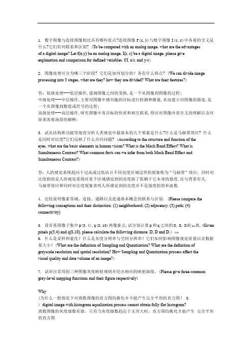
1.数字图像与连续图像相比具有哪些优点?连续图像f(x,y)与数字图像I(c,r)中各量的含义是什么?它们有何联系和区别? (To be compared with an analog image, what are the advantagesof a digital image? Let f(x,y) be an analog image, I(r, c) be a digital image, please giveexplanation and comparison for defined variables: f/I, x/r, and y/c)2.图像处理可分为哪三个阶段? 它们是如何划分的?各有什么特点? (We can divide image processing into 3 stages, what are they? how they are divided? What are their features?)答:低级处理---低层操作,强调图像之间的变换,是一个从图像到图像的过程;中级处理---中层操作,主要对图像中感兴趣的目标进行检测和测量,从而建立对图像的描述,是一个从图像到数值或符号的过程;高级处理---高层操作,研究图像中各目标的性质和相互联系,得出对图像内容含义的理解以及对原来客观场景的解释;3.试从结构和功能等角度分析人类视觉中最基本的几个要素是什么?什么是马赫带效应? 什么是同时对比度?它们反映了什么共同问题? (According to the structure and function of theeyes, what are the basic elements in human vision? What is the Mach Band Effect? What is Simultaneous Contrast? What common facts can we infer from both Mach Band Effect and Simultaneous Contrast?)答:人的视觉系统趋向于过高或过低估计不同亮度区域边界的现象称为“马赫带”效应;同时对比度指的是人的视觉系统对某个区域感觉到的亮度除了依赖于它本身的强度,还与背景有关. 马赫带效应和同时对比度现象表明人所感觉到的亮度并不是强度的简单函数.4.比较说明像素邻域、连接、通路以及连通基本概念的联系与区别。
电大一网一《数字与图像处理》2023春季学期数字与图像处理第2次平时作业-100分
新疆开放大学直属《数字与图像处理》2023春季学期数字与图像处理第2
次平时作业-100分
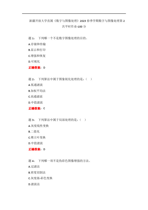
题1:下列哪一个不是数字图像处理的目的。
A.存储和传输
B.显示和打印
C.增强和恢复
D.可视化
正确答案:D
题2:下列算法中属于图象锐化处理的是:()
A.低通滤波
B.加权平均法
C.高通滤波
D.中值滤波
正确答案:C
题3:下列算法中属于局部处理的是:()
A.灰度线性变换
B.二值化
C.傅立叶变换
D.中值滤波
正确答案:D
题4:下列哪一项不是伪彩色图像增强的方法。
A.过滤法
B.密度切割法
C.灰度级-彩色变换
D.滤波法。
《数字图像处理》作业题目

数字图像处理作业班级:Y100501姓名:**学号:*********一、编写程序完成不同滤波器的图像频域降噪和边缘增强的算法并进行比较,得出结论。
频域降噪。
对图像而言,噪声一般分布在高频区域,而图像真是信息主要集中在低频区,所以,图像降噪一般是利用低通滤波的方法来降噪。
边缘增强。
图像的边缘信息属于细节信息,主要由图像的高频部分决定,所以,边缘增强一般采取高通滤波,分离出高频部分后,再和原频谱进行融合操作,达到边缘增强,改善视觉效果,或者为进一步处理奠定基础的目的。
1频域降噪,主程序如下:I=imread('lena.bmp'); %读入原图像文件J=imnoise(I,'gaussian',0,0.02);%加入高斯白噪声A=ilpf(J,0.4);%理想低通滤波figure,subplot(222);imshow(J);title('加噪声后的图像');subplot(222);imshow(A);title('理想低通滤波');B=blpf(J,0.4,4);%巴特沃斯低通滤波subplot(223);imshow(B);title('巴特沃斯低通滤波');C=glpf(J,0.4);%高斯低通滤波subplot(224);imshow(C);title('高斯低通滤波');用到的滤波器函数的程序代码如下:function O=ilpf(J,p) %理想低通滤波,p是截止频率[f1,f2]=freqspace(size(J),'meshgrid');hd=ones(size(J));r=sqrt(f1.^2+f2.^2);hd(r>p)=0;y=fft2(double(J));y=fftshift(y);ya=y.*hd;ya=ifftshift(ya);ia=ifft2(ya);O=uint8(real(ia));function O=blpf(J,d,n) %巴特沃斯低通滤波器,d是截止频率,n是阶数[f1,f2]=freqspace(size(J),'meshgrid');hd=ones(size(J));r=f1.^2+f2.^2;for i=1:size(J,1)for j=1:size(J,2)t=r(i,j)/(d*d);hd(i,j)=1/(t^n+1);endendy=fft2(double(J));y=fftshift(y);ya=y.*hd;ya=ifftshift(ya);ia=ifft2(ya);O=uint8(real(ia));function O=glpf(J,D) %高斯滤波器,D是截止频率[f1,f2]=freqspace(size(J),'meshgrid');r=f1.^2+f2.^2;Hd=ones(size(J));for i=1:size(J,1)for j=1:size(J,2)t=r(i,j)/(D*D);Hd(i,j)=exp(-t);endendY=fft2(double(J));Y=fftshift(Y);Ya=Y.*Hd;Ya=ifftshift(Ya);ia=ifft2(Ya);O=uint8(real(ia));运行结果如图1所示。
数字图像处理第二次作业
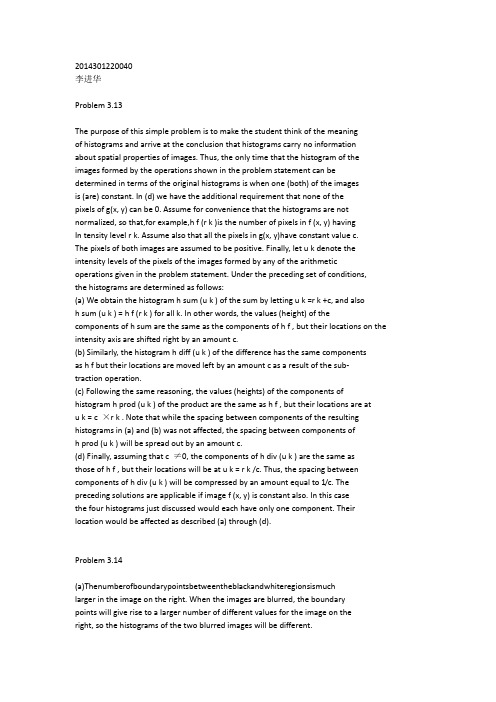
2014301220040李进华Problem 3.13The purpose of this simple problem is to make the student think of the meaningof histograms and arrive at the conclusion that histograms carry no informationabout spatial properties of images. Thus, the only time that the histogram of the images formed by the operations shown in the problem statement can be determined in terms of the original histograms is when one (both) of the imagesis (are) constant. In (d) we have the additional requirement that none of thepixels of g(x, y) can be 0. Assume for convenience that the histograms are not normalized, so that,for example,h f (r k )is the number of pixels in f (x, y) havingIn tensity level r k. Assume also that all the pixels in g(x, y)have constant value c.The pixels of both images are assumed to be positive. Finally, let u k denote the intensity levels of the pixels of the images formed by any of the arithmetic operations given in the problem statement. Under the preceding set of conditions,the histograms are determined as follows:(a) We obtain the histogram h sum (u k ) of the sum by letting u k =r k +c, and alsoh sum (u k ) = h f (r k ) for all k. In other words, the values (height) of the components of h sum are the same as the components of h f , but their locations on the intensity axis are shifted right by an amount c.(b) Similarly, the histogram h diff (u k ) of the difference has the same componentsas h f but their locations are moved left by an amount c as a result of the sub-traction operation.(c) Following the same reasoning, the values (heights) of the components of histogram h prod (u k ) of the product are the same as h f , but their locations are atu k = c ×r k . Note that while the spacing between components of the resulting histograms in (a) and (b) was not affected, the spacing between components ofh prod (u k ) will be spread out by an amount c.(d) Finally, assuming that c ≠0, the components of h div (u k ) are the same asthose of h f , but their locations will be at u k = r k /c. Thus, the spacing between components of h div (u k ) will be compressed by an amount equal to 1/c. The preceding solutions are applicable if image f (x, y) is constant also. In this casethe four histograms just discussed would each have only one component. Their location would be affected as described (a) through (d).Problem 3.14(a)Thenumberofboundarypointsbetweentheblackandwhiteregionsismuchlarger in the image on the right. When the images are blurred, the boundarypoints will give rise to a larger number of different values for the image on theright, so the histograms of the two blurred images will be different.(b) To handle the border effects, we surround the image with a border of 0s. We assume that image is of size N ×N (the fact that the image is square is evident from the right image in the problem statement). Blurring is implemented bya 3×3 mask whose coefficients are 1/9. Figure P3.14 shows the different typesof values that the blurred left image will have (see image in the problem statement). The values are summarized in Table P3.14-1. It is easily verified that thesum of the numbers on the left column of the table is N 2 . A histogram is easily constructed from the entries in this table. A similar (tedious) procedure yieldsthe results in Table P3.14-2.Problem 3.16(a)The key to solving this problem is to recognize (1) that the convolution resultat any location (x,y) consists of centering the mask at that point and then formingthesumoftheproductsofthemaskcoefficientswiththecorrespondingpixels in the image; and (2) that convolution of the mask with the entire image results in every pixel in the image being visited only once by every element ofthe mask (i.e., every pixel is multiplied once by every coefficient of the mask). Because the coefficients of the mask sum to zero, this means that the sum of the products of the coefficients with the same pixel also sum to zero. Carrying outthis argument for every pixel in the image leads to the conclusion that the sumof the elements of the convolution array also sum to zero.(b) The only difference between convolution and correlation is that the maskis rotated by 180 ◦. This does not affect the conclusions reached in (a), so cor- relating an image with a mask whose coefficients sum to zero will produce acorrelation image whose elements also sum to zero.Problem 3.17One of the easiest ways to look at repeated applications of a spatial filter is to use superposition. Let f (x, y) and h(x, y) denote the image and the filter function, respectively. Assuming square images of size N ×N for convenience, we can express f (x, y) as the sum of at most N 2 images, each of which has only one nonzero pixel (initially, we assume that N can be infinite). Then, the process of running h(x, y) over f (x, y) can be expressed as the following convolution:h(x,y) ★f (x,y) =h(x,y) ★[f1 (x,y)+ f 2 (x,y)+···+ f N 2 (x,y)]Suppose for illustrative purposes that f i (x,y) has value 1 at its center, while the other pixels are valued 0, as discussed above (see Fig. P3.17a). If h(x,y) is a3×3 mask of 1/9’s (Fig. P3.17b), then convolving h(x,y) with f i (x,y) will produce an image with a 3×3 array of 1/9’s at its center and 0s elsewhere, as Fig.P3.17(c) shows. If h(x,y) is now applied to this image, the resulting image willbe as shown in Fig. P3.17(d). Note that the sum of the nonzero pixels in both Figs. P3.17(c) and (d) is the same, and equal to the value of the original pixel. Thus, it is intuitively evident that successive applications of h(x,y) will ”diffuse”the nonzero value of f i (x,y) (not an unexpected result, because h(x,y)is a blurring filter). Since the sum remains constant, the values of the nonzero elements will become smaller and smaller, as the number of applications of the filter increases. The overall result is given by adding all the convolved f k (x,y),for k =1,2,...,N 2 .It is noted that every iteration of blurring further diffuses the values out- wardly from the starting point. In the limit, the values would get infinitely small, but, because the average value remains constant, this would require an image of infinite spatial proportions. It is at this junction that border conditions become important. Although it is not required in the problem statement, it is instructive to discuss in class the effect of successive applications of h(x,y) to an image of finite proportions. The net effect is that, because the values cannot diffuse out- ward past the boundary of the image, the denominator in the successive appli- cationsofaveragingeventuallyoverpowersthepixelvalues, driving the image to zero in the limit. A simple example of this is given in Fig. P3.17(e), which shows an array of size 1×7 that is blurred by successive applications of the 1×3 mask h(y) =13 [1,1,1]. We see that, as long as the values of the blurred 1 can diffuseout, the sum,S, of the resulting pixels is 1. However, when the boundary is met, an assumption must be made regarding how mask operations on the border are treated. Here, we used the commonly made assumption that pixel value imme- diately past the boundary are 0. The mask operation does not go beyond the boundary, however. In this example, we see that the sum of the pixel values be- gins to decrease with successive applications of the mask. In the limit, the term 1/(3) n would overpower the sum of the pixel values, yielding an array of 0s.Problem 3.21From Fig. 3.33 we know that the vertical bars are 5 pixels wide, 100 pixels high, and their separation is 20 pixels. The phenomenon in question is related to the horizontal separation between bars, so we can simplify the problem by consid- ering a single scan line through the bars in the image. The key to answering this question lies in the fact that the distance (in pixels) between the onset of one bar and the onset of the next one (say, to its right) is 25 pixels.Consider the scan line shown in Fig. P3.21. Also shown is a cross sectionof a 25×25 mask. The response of the mask is the average of the pixels that it encompasses. We note that when the mask moves one pixel to the right, it loses one value of the vertical bar on the left, but it picks up an identical one on the right, so the response doesn’t change. In fact, the number of pixels belonging to the vertical bars and contained within the mask does not change, regardless of where the mask is located (as long as it is contained within the bars, and not near the edges of the set of bars).The fact that the number of bar pixels under the mask does not change is dueto the peculiar separation between bars and the width of the lines in relationto the 25-pixel width of the mask This constant response is the reason why no white gaps are seen in the image shown in the problem statement. Note that this constantresponsedoesnothappenwiththe23×23orthe45×45masksbecause they are not ”synchronized”with the width of the bars and their separation.Problem 3.23The student should realize that both the Laplacian and the averaging process are linear operations, so it makes no difference which one is applied first.。
《数字图像处理》习题参考附标准答案
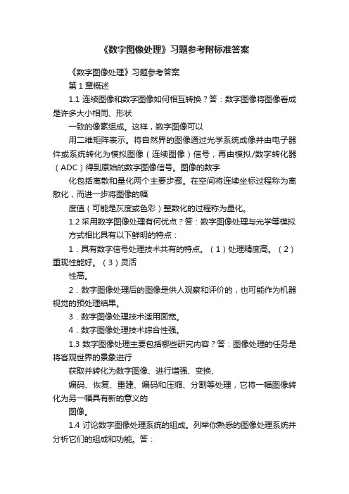
《数字图像处理》习题参考附标准答案《数字图像处理》习题参考答案第1章概述1.1连续图像和数字图像如何相互转换?答:数字图像将图像看成是许多大小相同、形状一致的像素组成。
这样,数字图像可以用二维矩阵表示。
将自然界的图像通过光学系统成像并由电子器件或系统转化为模拟图像(连续图像)信号,再由模拟/数字转化器(ADC)得到原始的数字图像信号。
图像的数字化包括离散和量化两个主要步骤。
在空间将连续坐标过程称为离散化,而进一步将图像的幅度值(可能是灰度或色彩)整数化的过程称为量化。
1.2采用数字图像处理有何优点?答:数字图像处理与光学等模拟方式相比具有以下鲜明的特点:1.具有数字信号处理技术共有的特点。
(1)处理精度高。
(2)重现性能好。
(3)灵活性高。
2.数字图像处理后的图像是供人观察和评价的,也可能作为机器视觉的预处理结果。
3.数字图像处理技术适用面宽。
4.数字图像处理技术综合性强。
1.3数字图像处理主要包括哪些研究内容?答:图像处理的任务是将客观世界的景象进行获取并转化为数字图像、进行增强、变换、编码、恢复、重建、编码和压缩、分割等处理,它将一幅图像转化为另一幅具有新的意义的图像。
1.4讨论数字图像处理系统的组成。
列举你熟悉的图像处理系统并分析它们的组成和功能。
答:如图1.8,数字图像处理系统是应用计算机或专用数字设备对图像信息进行处理的信息系统。
图像处理系统包括图像处理硬件和图像处理软件。
图像处理硬件主要由图像输入设备、图像运算处理设备(微计算机)、图像存储器、图像输出设备等组成。
软件系统包括操作系统、控制软件及应用软件等。
图1.8 数字图像处理系统结构图11.5常见的数字图像处理开发工具有哪些?各有什么特点?答.目前图像处理系统开发的主流工具为Visual C++(面向对象可视化集成工具)和MATLAB 的图像处理工具箱(ImageProcessingToolbox)。
两种开发工具各有所长且有相互间的软件接口。
《数字图像处理》课后作业2015
《数字图像处理》课后作业(2015)第2章2.5一个14mm⨯14mm的CCD摄像机成像芯片有2048⨯2048个像素,将它聚焦到相距0.5m远的一个方形平坦区域。
该摄像机每毫米能分辨多少线对?摄像机配备了一个35mm镜头。
(提示:成像处理模型见教材图2.3,但使用摄像机镜头的焦距替代眼睛的焦距。
)2.10高清电视(HDTV, High Definition TV )使用1080条水平电视线(TV Line)隔行扫描来产生图像(每隔一行在显像管表面画出一条水平线,每两场形成一帧,每场用时1/60秒,此种扫描方式称为1080i,即1080 interlace scan;对应的有1080p,即1080 progressive scan,逐行扫描)。
图像的宽高比是16:9。
水平电视线数(水平行数)决定了图像的垂直分辨率,即一幅图像从上到下由多少条水平线组成;相应的水平分辨率则定义为一幅图像从左到右由多少条垂直线组成,水平分辨率通常正比于图像的宽高比。
一家公司已经设计了一种图像获取系统,该系统由HDTV图像生成数字图像,彩色图像的每个像素都有24比特的灰度分辨率(红、绿、蓝分量各8比特)。
请计算不压缩时存储90分钟的一部HDTV电影所需要的存储容量。
2.22图像相减常用于在产品装配线上检测缺失的元件。
方法是事先存储一幅对应于正确装配的产品图像,称为“金”图像(“golden” image),即模板图像。
然后,在同类型产品的装配过程中,采集每一装配后的产品图像,从中减去上述模板图像。
理想情况下,如果产品装配正确,则两幅图像的差值应为零。
而对于缺失元件的产品,其图像与模板图像在缺失元件区域不同,两幅图像的差值在这些区域就不为零。
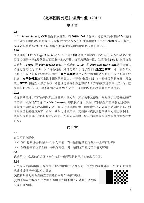
在实际应用中,您认为需要满足哪些条件这种方法才可行?第3章3.5在位平面分层中,(a)如果将低阶位平面的一半设为零值,对一幅图像的直方图大体上有何影响?(b)如果将高阶位平面的一半设为零值,对一幅图像的直方图又有何影响?3.6试解释为什么离散直方图均衡化技术一般不能得到平坦的输出直方图。
- 1、下载文档前请自行甄别文档内容的完整性,平台不提供额外的编辑、内容补充、找答案等附加服务。
- 2、"仅部分预览"的文档,不可在线预览部分如存在完整性等问题,可反馈申请退款(可完整预览的文档不适用该条件!)。
- 3、如文档侵犯您的权益,请联系客服反馈,我们会尽快为您处理(人工客服工作时间:9:00-18:30)。
实验报告
实验名称实验二空间域数字图像增强
实验课程数字图像处理
姓名成绩
班级学号
日期 2011年11月20日地点综合试验楼
1.实验目的
(1)了解空间域图像增强的各种方法(点处理、掩模处理); (2)通过编写程序掌握采用直方图均衡化进行图像增强的方法;
(3)使用邻域平均法编写程序实现图像增强,进一步掌握掩模法及其改进(加门限法) 消除噪声的原理;
(4)总结实验过程(实验报告,左侧装订):方案、编程、调试、结果、分析、结论。
2.实验环境(软件、硬件及条件)
Windws2000/XP 、MA TLAB 6.x or above 、V isual C++、Visual Basic 或其它
3.实验方法
对如图所示的两幅128×128、256级灰度的数字图像fing_128.img 和cell_128.img 进行如下处理:
(1)对原图像进行直方图均衡化处理,同屏显示处理前后图像及其直方图,比较异同,
并回答为什么数字图像均衡化后其直方图并非完全均匀分布。
(2)对原图像加入点噪声,用4-邻域平均法平滑加噪声图像(图像四周边界不处理,下同),同屏显示原图像、加噪声图像和处理后的图像。
①不加门限; ②加门限),(2
1n m f T
=,
(其中∑∑=i
j
j i f N
n m f )
,(1),(2
)
4.实验分析
(1)直方图均衡化处理
本题的关键步骤在于对灰度出现频率的概率统计,利用如下函数实现:
for x=1:128
指纹图fing_128.img
显微医学图像cell_128.img
for y=1:128
q(f(x,y)+1)=q(f(x,y)+1)+1;
end
end
在概率统计完成之后,做出其累计直方图:
t(1)=s(1);
for i=2:256
t(i)=t(i-1)+s(i);
end
subplot(2,1,1);
bar(X,t');
然后用 t0=floor(255*t+0.5)函数将概率累计直方图变为对灰度级频数的累计,这样就得到了不同灰度级对应的不同的频数。
最后通过以下函数将概率分布均衡到各个不同的灰度级上去:原理为对于频数累计直方图变化的快慢分配给以不同的频率,在频数累计图变化慢的地方会分配给相对较多的频率,而对于频数累计直方图变化较快的地方则分配给较少的频率,这样便实现了直方图的均衡化。
t1=zeros(1,256);
for i=1:256
t1(t0(i)+1)=s(i)+t1(t0(i)+1);
end
(2)图像加入噪声及去噪
利用如下函数将噪声加入到原图像中:
a=randn(128,128);
f=a*30+fg;
利用四邻域平滑法对图像进行平滑处理,并且不加门限:
f0=f;
for x=2:127
for y=2:127
f0(x,y)=(f((x-1),y)+f((x+1),y)+f(x,(y-1))+f(x,(y+1)))./4;
end
end
第二次平滑处理时加入门限,设定方法为:
t=0;
for x=1:128
for y=1:128
t=t+f0(x,y);
end
end
T=t/(128^2*2);
利用如下的循环函数实现对图像的加门限平滑,注意的是x、y的起止范围,四周的点不作处理。
f1=f;
for x=2:127
for y=2:127
h=(f((x-1),y)+f((x+1),y)+f(x,(y-1))+f(x,(y+1)))./4;
if abs(f(x,y)-h)>T
f1(x,y)=h;
else
f1(x,y)=f(x,y);
end
end
end
5.实验结果及结论
(1)直方图均衡化处理
原始图像及灰度级概率分布图
频率及频数统计分布直方图
图像均衡化之后的结果
实验结论:
由于原图像中目标物的灰度主要集中于低亮度部分,而且象素总数比较多,经过直方
图均衡后,目标物的所占的灰度等级得到扩展,对比度加强,使整个图像得到增强。
原始图像及灰度级概率分布图
频率及频数统计分布直方图
图像均衡化之后的结果
实验结论:
由于原图像中目标物的灰度主要集中于低亮度部分,而且象素总数比较少,而所占的灰度等级比较多,因此图像的对比度比较好,亮度比较大,整体图像清晰。
经过直方图均衡后,目标物的所占的灰度等级被压缩,对比度减弱,反而使目标物变的难以辨认。
数字图像均衡化后,其直方图并非完全均匀分布,这是因为图像的象素个数和灰度等级均为离散值;而且均衡化使灰度级并归,因此,均衡化后,其直方图并非完全均匀分布。
(2)图像加入噪声及去噪
原始图像、加噪图像、不加门限的平滑以及加入门限的平滑图像
原始图像、加噪图像、不加门限的平滑以及加入门限的平滑图像实验结论:
可以看到,对加噪图像进行4-邻域平滑后,去处了大部分的噪声,但也使目标物边缘变的模糊。
加门限后,目标物的边缘得到加强。
附件:
(1)直方图均衡化处理源程序
clc;
fid=fopen('D:\images\fing_128.img','r');
f=fread(fid,[128,128],'uchar');
subplot(2,1,1);
imshow(f,[0,255]);
q=zeros(1,256);
for x=1:128
for y=1:128
q(f(x,y)+1)=q(f(x,y)+1)+1;
end
end
s=q./(128*128);
X=0:255;
subplot(2,1,2);
bar(X,s','g');
figure;
t=zeros(1,256);
t(1)=s(1);
for i=2:256
t(i)=t(i-1)+s(i);
end
subplot(2,1,1);
bar(X,t');
t0=floor(255*t+0.5);
subplot(2,1,2);
bar(X,t0');
figure;
t1=zeros(1,256);
for i=1:256
t1(t0(i)+1)=s(i)+t1(t0(i)+1);
end
subplot(2,1,2);
bar(X,t1','g');
f1=zeros(128,128)
for x=1:128
for y=1:128
f1(x,y)=t0(f(x,y)+1);
end
end
subplot(2,1,1);
imshow(f1,[0,255]);
(2)图像加入噪声及去噪的源程序
clc;
fid=fopen('D:\images\cell_128.img','r');
fg=fread(fid,[128,128],'uchar');
subplot(2,2,1);
imshow(fg,[0,255]);
a=randn(128,128);
f=a*30+fg;
subplot(2,2,2);
imshow(f,[0,255]);
f0=f;
for x=2:127
for y=2:127
f0(x,y)=(f((x-1),y)+f((x+1),y)+f(x,(y-1))+f(x,(y+1)))./4;
end
end
subplot(2,2,3);
imshow(f0,[0,255]);
t=0;
for x=1:128
for y=1:128
t=t+f0(x,y);
end
end
T=t/(128^2*2);
f1=f;
for x=2:127
for y=2:127
h=(f((x-1),y)+f((x+1),y)+f(x,(y-1))+f(x,(y+1)))./4;
if abs(f(x,y)-h)>T
f1(x,y)=h;
else
f1(x,y)=f(x,y);
end
end
end
subplot(2,2,4);
imshow(f1,[0,255]);。