Majorana Spin-Flip Transition of Atom in Varying Magnetic Field(1932)
Nature of the spin dynamics and 13 magnetization plateau in azurite
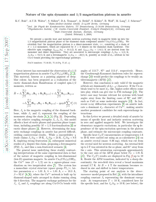
angles of 113.7◦ , 97◦ and 113.4◦, respectively. Hence, the Goodenough-Kanamori-Anderson rules for superexchange [10] would predict the couplings to be weakly antiferromagnetic (AFM) [11]. However, this conclusion is only valid if the magnetic orbitals are dominantly of dx2 −y2 character. If the Cu orbitals tend to be more dz2 like, higher-order effects come into play, which can give rise to FM exchange [12]. The latter case may become relevant for systems with bond angles away from the limiting cases of 90◦ and 180◦ , such as CuO or some molecular magnets [13]. In fact, recent x-ray diffraction experiments [9] on azurite indicate a dominant dz2 character of Cu2+ , making azurite another prominent candidate for such superexchange interactions. In this Letter we present a detailed study of azurite by means of specific heat and inelastic neutron scattering in zero and applied magnetic field. We investigate the elementary magnetic excitations, in particular the q dependence of the spin-excitation spectrum in the plateau phase, and estimate the microscopic coupling constants. Specific heat Cp (T ) measurements at temperatures 1.6 to 30 K were carried out using an ac-calorimeter [14] on an azurite crystal (mass: 0.36 mg), which was cut from the crystal used for neutron scattering. An external field up to 4 T was oriented in the ac-plane, and 65◦ away from the c axis. This orientation corresponds approximately to the easy axis of the AFM phase below TN = 1.85 K [15]. The Cp (T ) results are displayed in Fig. 1 up to 10 K. Beside the AFM transition, indicated by a sharp discontinuity, the zero-field data reveal a broad maximum around 3.7 K. At B = 4 T the maximum becomes reduced in size and shifted to lower temperatures. The starting point of our analysis is the dimermonomer model proposed in Ref. [4], with the intradimer coupling constant J2 representing the dominant energy scale. At temperatures T < 10 K, considered here for the specific heat, and for J2 /kB ≫ 10 K (see below), the
清华考博辅导:清华大学计算机科学与技术考博难度解析及经验分享

清华考博辅导:清华大学计算机科学与技术考博难度解析及经验分享根据教育部学位与研究生教育发展中心最新公布的第四轮学科评估结果可知,全国共有168所开设计算机科学与技术专业的大学参与了2017-2018计算机科学与技术专业大学排名,其中排名第一的是北京大学,排名第二的是清华大学,排名第三的是浙江大学。
作为清华大学实施国家“211工程”和“985工程”的重点学科,计算机科学与技术一级学科在历次全国学科评估中均名列第二。
下面是启道考博整理的关于清华大学计算机科学与技术考博相关内容。
一、专业介绍计算机科学与技术是研究计算机的设计与制造,并利用计算机进行有关的信息表示、收发、存储、处理、控制等的理论方法和技术的学科。
计算机专业涵盖计算机科学与技术、计算机软件工程、计算机信息工程等专业,主要培养具有良好的科学素养,系统地、较好地掌握计算机科学与技术,包括计算机硬件和软件组成原理、计算机操作系统、计算机网络基础、算法与数据结构等,计算机的基本知识和基本技能与方法,能在科研部门、教育、企业、事业、行政管理部门等单位从事计算机教学、科学研究和计算机科学与技术学科的应用。
清华大学计算机科学与技术专业在博士招生方面,划分为3个研究方向:081200计算机科学与技术研究方向:01信息安全;02机器智能;03金融科技;04网络科学;05计算生物学;06能源信息科学;07机器人;08理论计算机科学;09量子信息此专业实行申请考核制。
二、考试内容清华大学计算机科学与技术专业博士研究生招生为资格审查加综合考核形式,由笔试+面试构成。
其中,综合考核内容为:综合考核形式为面试:每位考生约30 分钟,满分100 分。
面试重点考查申请人在本学科攻读博士学位的基本素养、学术能力、学术志趣等。
三、时间安排1.博士生申请在每年的8-9月和11月。
2.直博生(包括夏令营拟录取的直博生)、硕博连读生及部分9月份招收普博生的院系8-9月申请,9月中下旬考试录取,见当年招生简章及目录、招生说明、直博直硕招生要求。
CALPHAD软件介绍
Abstract
The phase-field method has become an important and extremely versatile technique for simulating microstructure evolution at the mesoscale. Thanks to the diffuse-interface approach, it allows us to study the evolution of arbitrary complex grain morphologies without any presumption on their shape or mutual distribution. It is also straightforward to account for different thermodynamic driving forces for microstructure evolution, such as bulk and interfacial energy, elastic energy and electric or magnetic energy, and the effect of different transport processes, such as mass diffusion, heat conduction and convection. The purpose of the paper is to give an introduction to the phase-field modeling technique. The concept of diffuse interfaces, the phase-field variables, the thermodynamic driving force for microstructure evolution and the kinetic phase-field equations are introduced. Furthermore, common techniques for parameter determination and numerical solution of the equations are discussed. To show the variety in phase-field models, different model formulations are exploited, depending on which is most common or most illustrative. c 2007 Elsevier Ltd. All rights reserved.
20111219_固态转变-非扩散型相变

马氏体相变晶体学
晶体学唯像理论
唯像理论:phenomenological theory, 一类具有 很大的普适性但不涉及细节的理论。 马氏体相变的晶体学唯像理论,只规定了转变前 后的晶体学关系,不能说明转变的机制或原子过 程。 不能用于求两相的点阵类型和点阵常数。 原则上可用于求得惯习面、点阵取向关系、总应 变量、简单切变量及相晶面的空间取向。
马氏体转变基本概念
不变平面特征
一般不变平面
s
s
(a) 简单拉伸
(b) 简单切变
(c) 一般性不变平面应变
uniaxial dilatation
simple shear
general invariantplane strain
马氏体转变基本概念
不变平面特征 /形状改变 /表面浮凸
马氏体相变的平面不变应变,由均匀的Bain畸变(得到马氏体晶体结构)、均匀 的旋转和不均匀的简单切变(后二者为了保证不转动不畸变的不变平面)构成。
马氏体相变的其它派生特征
马氏体与母相之间存在严格的晶体学关系,相界面为共格 或半共格。 惯习面(habit plane)现象:马氏体沿母相某特定晶面 析出。 新旧相成分相同。 多种马氏体相变:变温马氏体相变,等温马氏体相变,热 弹性马氏体相变,应力诱发马氏体相变,爆发马氏体相 变,… …
马氏体转变基本概念
马氏体相变的定义
替换原子经无扩散位移(均匀和不均匀形变) 由此产生形 状改变和表面浮突, 呈不变平面特征的一级、形核- 长大 型的相变。 ---徐祖耀 Shear-dominant, lattice-distortive, diffusionless transformation occurring by nucleation and growth* --- J.W. Christian, G.B. Olson and M. Cohen Martensite is best defined not by what it is, but by how it forms. ---- Morris Cohen (MIT)
一维磁性原子链系统中的Majorana费米子态

一维磁性原子链系统中的Majorana费米子态杨双波【摘要】对处于螺旋形磁场及横向均匀磁场的一维磁性原子链模型,在平均场近似下通过自洽地求解Bogoliubov-de-Genes方程我们计算了系统的能谱.我们发现在一定参数值的范围内能谱随螺旋形磁场振幅值演化呈现能量为零的Majorana 费米子态.我们计算了局域态密度发现对Majorana费米子其态密度的峰值出现在链的两端(或中点)位置.我们计算了波函数其空间分布,发现它与局域态密度的结果一致.%For a model of one dimensional magnetic atomic chain in both a helical magnetic field and a transverse uniform magnetic field,we calculate its energy spectrum by solving Bogoliubov-de-Genes equation selfconsistently in the mean field approximation. We find that for a certain parameter setting,energy spectrum evolving with amplitude of helical magnetic field,appears Majorana fermion eigenstates. We calculate local density of states,and find that the local density of states for Majorana fermion shows peaks at the both ends(or at middle)of the magnetic atomic chain. We calculate wave function,and its spatial distribution agrees with local density of states.【期刊名称】《南京师大学报(自然科学版)》【年(卷),期】2017(040)003【总页数】8页(P110-117)【关键词】Majorana费米子;磁性原子链;BdG方程;局域态密度【作者】杨双波【作者单位】南京师范大学物理科学与技术学院,江苏省大规模复杂系统数值模拟重点实验室,江苏南京210023【正文语种】中文【中图分类】O413.1Majorana fermion[1] which is a particle of the same as its own antiparticle,has been attracting great attention. Firstly,because of Majorana fermion being connected with topological phase concept,secondly because of its topological character,it provides a platform of potential application in topological quantum computing and quantum storing[2-4]. So experimentally and theoretically search for physical system of Majorana fermion has been a very hot research topic. The purpose of all these researches is to generate a topological superconductor,so that the Majorana fermion appears as a single excitation at the boundary. Recently,Majorana fermion has been studied for a model of an atomic chain in a helical magnetic field in close proximity to a s-wave superconductor[5-7],and the result shows that at a certain parameter setting,the Majorana fermion is localized at the both end of the magnetic atomic chain. This is a spatially uniform system,after a gauge transformation,the Hamiltonian of the system will become an invariant form for space displacement. In this paper we modified this system by adding a new Zeeman term in the original Hamiltonian,which correspondsto a uniform magnetic field h perpendicular to the atomic chain being applied to the original system. Because of the new Zeeman term,the system is nonuniform spatially,we will study the structure of the Majorana fermion for the system of h≠0.In this paper,we get the system eigenenergies and eigenvectors by numerically solving BdG equation,and then we study the birth and the localization in space of the Majorana fermion by calculating the spatially resolved local density of states and wave function. The structure of the paper is as the following,the Model and theory is in section 1,the result of numerical calculation and discussion is in section 2,the summary of the paper is in section 3.Consider a N-atom atomic chain in a helical magnetic filed or magnetic structure. The magnetic filed at site n is =B0(cosnθ+sinnθ),where θ is the angle made by the magnetic fields at the adjacent sites of the atomic chain,the whole atomic chain is in proximity to the surface of a s-wave superconductor,and in the transverse direction of the atomic chain a uniform magnetic field h is applied. The Hamiltonian of this magnetic atomic chain in mean field approximation is given byH=tx(cn+1α+h.c.)-μcnα+(cnβ+Δ(n)(+h.c.)+h(σz)ααcnα,where tx is the jumping amplitude for electron between two adjacent sites,μ is chemical potential,Δ(n)is the superconductor pairing potential or order parameter at sit n,h is the weak uniform magnetic field for tuning system energy spectrum. or cnα is the operator to creat or annihilate an electron of spin α respectively at site n, is pauli matrix vec tor,and h.c. standfor complex conjugate. By introducing Nambu spinor representationψi=(ci↑,ci↓,,-)T,then Hamiltonian(1)can be written as BdG form,i.e.H=Hijψj,where Hij is the BdG Hamiltonian at site i,which can be written as where Kij=tx(δi+1,j+δi-1,j)-μδij,γij=(h-B0cosiθ)δij. This is a 4N×4N matrix,whose energy eigenvalue εn and eigenfunctionψn(i)=(un(↑,i),un(↓,i),vn(↓,i),vn(↑,i))T, for i=1,2,…,N,is determined by eigenvalue equationand boundary condition. In mean field approximation the order parameter at site i takes the form[8]and the mean number of electron at site i iswhere fn=1/(1+eεn/kBT) is the Fermi distribution,T is temperature in Kelvin. The total number of electron isincluding spin up and spin down electrons. To determine eigenenergy,eigenfunction,order parameter,we need to selfconsistently solve eigenvalue equation(3)with(4)-(6). In this paper,we deal with the case of temperature T=0,then the order parameter and the mean number of electron in site i are given bySpecial case:h=0 and Δ(i)=Δ0,a constant. The Hamiltonian in(1)can be transformed into spatially unform form by a gauge transformation. The topologically nontrivial region of the parameter set is given bywhere Majorana fermion corresponds to εn=0. As |h|≠0,Hamiltonian in(1)is nonuniform in space,and the nontrivial region of parameter set can not be obtained analytically.In this paper we deal with open boundary condition with and without themiddle magnetic domain wall,and at the magnetic domain wall we replace θ by -θ. We have also studied under the periodic boundary condition,and found the result has no significant changes.We first study the character of the Majorana fermion as the order parameter Δ and chemical potential μ are constants,then we study the influence of nonuniform Δ(i)on the result of Majorana fermion by doing selfconsistent calculation. In calculation,we choose the number of site N for the atomic chain according to the angle θ,so that the magnetic field at the both ends of the atomic chain points to the same direction.2.1 Energy Spectrum and Wave FunctionsFor a one-dimensional magnetic atomic chain with magnetic domain wall in the middle,the parameter set is chosen asΔ0=1.0,tx=1.0,μ=2.5,h=0.1,θ=π/2,and length of the chain is chosen asN=81 sites. For every value of B0 in the interval[1.0,4.0],we diagonalize the 4N×4N BdG Hamiltonian matrix(2),we get 4N energy eigenvalues and 4N eigenvectors. In open boundary condition,the energy spectrum is shown in Fig.1. For B0 in the interval[1.486 6,3.996 8],we can see that thereexists eigenstates whose eigenenergy εn=0,and these eigenstates are Majorana fermions. The interval for the existense of Majorana fermion in the case of h=0.1 is very close to the interval[1.476,4.039]calculatedfrom(9)for the h=0 case. For Majorana fer mion at B0=2.1,εn=0,shown in red dot in Fig.1,we calculate its wave functionun(↑,i),un(↓,i),vn(↑,i),vn(↓,i),the result is shown in Fig.2(a-d). We can see that the amplitude of the wave function concentrates on the both ends and themiddle of the atomic chain. In Fig.3,we show wave function for the same magnetic atomic chain without magnetic domain wall in the middle,the amplitude of the wave function concentrates on both ends of the magnetic atomic chain. This is similar to the previous result for the 1-dimensional magnetic atomic chain without uniform magnetic field,h=0.2.2 Local Density of States and Total Density of StatesIn this subsection,we study the space distribution of density ofstates(DOS),which is called local density of states(LDOS)and is defined as ρ(ε,i)is a function of energy and space position,and the total density of states(TDOS)can be written as,i.e.,the arithmetic mean of local density of states,a function of energy only. In numerical calculation,we replace δ by a Lorentz function. Fo r parameter setting h=0.1,tx=1.0,Δ=1.0,μ=2.5,θ=π/2,N=81,and B0=2.1,the local density of states for a Majorana fermion and the mean number of electrons on each site are shown in Fig.4(a-d)for the magnetic atomic chain with magnetic domain wall in the middle. Fig.4(a)shows the local density of states ρ(ε,i)in a 3D-plot;Fig.4(b)shows the local density of states ρ(ε,i)in a 2D contour plot;Fig.4(c)shows the local density of states for Majorana fermion ρ(ε=0,i);Fig.4(d)shows the mean number of electron on each si te of atomic chain<n(i)>. We can see from the Fig.4 that the Majorana fermion is localized at two ends and middle for the magnetic atomic chain with magnetic domain wall in the middle. The mean number of electrons on each site of the atomic chain is around 1.5. In Fig.5(a-d)we show theresult for the same magnetic atomic chain without magnetic domain wall in the middle,then we see density of states for Majorana fermion is peaked only at both ends of the magnetic atomic chain.2.3 The Self-consistent ResultAs the order parameter Δ(i)is space position i dependent,we calculate the energy spectrum and local density of states by selfconsistently solving the eigenvalue equation(3)with equations(7)and(8). For parameter seth=0.1,tx=1.0,μ=2.5,U0=4.0,θ=π/2,N=81,the selfconsistently calculated energy spectrum is shown in Fig.6,the Majorana fermion region can be seen,is still there,but the interval is shorten. The local density of states and mean numbers of electron on each site for Majorana fermion at B0=1.57 are shown in Fig.7(a-d)and Fig.9(a-d). By comparison with Fig.4(a-d),we find the main characters are same,but peak position for selfconsistent result moved inside a little bit. We calculate the selfconsistent wave function for Majorana fermion,and the results are shown in Fig.8(a-d)and Fig.10(a-d). The amplitude is significiently large at both ends for magnetic atomic chain without magnetic domain wall,and significiently large at both ends and middle for a magnetic chain with magnetic domain wall in the middle. This agrees with the result of local density of states.In mean field approximation,and by numerically solving Bogoliubov-de-Genes(BdG)equation,this paper studies the birth,and the localization in space of the Majorana fermion in a one dimensional atomic chain in helical magnetic field,and a uniform magnetic field h which is perpendicular to the atomic chain. Studies find that at a certain parameter setting,theevolution of the energy spectrum with helical magnetic field amplitude B0 appears the zero energy eigenstates,which corresponding to the Majorana fermion. We calculate the local density of states,and find that the local density of states for the Majorana fermion has two peaks on the both end of the magnetic atomic chain. When a magnetic domain wall is applied at the middle of the maqgnetic atomic chain,the Majorana fermion shows peaks at both ends and the middle of the magnetic chain. As the order parameter is a function of space coordinate,we do selfconsistent calculation,and find that by comparing with the result of nonselfconsistent calculation,the energy spectrum and the shape of the local density of states are changed a little bit,but the main character does not change. [1] MAJORANA E. Symmetric theory of electron and positrons[J]. Nuovo Cimento,1937,14(1):171-181.[2] WILCZEK F. Majorana returns[J]. Nat Phys,2009,5(9):614-618.[3] NAYAK C,SIMON S H,STERN A,et al. Non-Abelian anyons and topological quantum computation[J]. Rev Mod Phys,2008,80(3):1 083-1 159.[4] ALICEA J. New directions in the persuit of Majorana fermions in solid state system[J]. Rep Prog Phys,2012,75(7):076501-1-36.[5] NADJ-PERGE S,DROZDOV I K,BERNEVIG B A,et al. Proposal for realizing Majorana fermions in chain of magnetic atoms on a superconductor [J]. Phys Rev B,2013,88(2):020407-1-5(R).[6] PÖYHÖNEN K,WESTSTRÖM A,RÖNTYNEN J,et al. Majorana state in helical shiba chain and ladders[J]. Phys Rev B,2014,89(11):115109-1-7.[7] VAZIFEH M M,FRANZ M. Self-organized topological state with Majorana fermions[J]. Phys Rev Lett,2013,111(20):206802-1-5.[8] SACRAMENTO P D,DUGAEV V K,VIEIRA V R. Magnetic impurities in a superconductors:effect of domainwall and interference[J]. Phys RevB,2007,76(1):014512-1-21.[9] EBISU H,YADA K,KASAI H,et al. Odd frequency pairing in topological superconductivity in a one dimensional magnetic chain[J]. Phys RevB,2015,91(5):054518-1-15.【相关文献】Received data:2016-11-17.Corresponding author:Yang Shuangbo,professor,majored in nonlinear physics and low dimensionalsystem.E-mail:*********************.cndoi:10.3969/j.issn.1001-4616.2017.03.016CLC number:O413.1 Document codeA Article ID1001-4616(2017)03-0110-08。
RAFT聚合合成功能化嵌段共聚物和聚合物接枝碳纳米管地研究

的多壁碳绒米管也有瞬撵验赛瑟自缎装幸亍鸯。这种横助于两亲的接棱聚会物实现
豹组装行为在其谴缡米粒子表露魏金粒子表霭也蠢残察到嘲。
H薛摊40l AFM妇姆瞒of tl站inl。£融ial laycf of EPMMA2皆SWa啊皆黔lAA船矗妇缸捌麟蠡鬣瞪d矗翱匝ch幻∞。|bn珏,钿撇f魏由I|融。
F置酣托4.12TEM imag髓of EPMMA2分MWa叮每·邶M九
合成的聚合物接枝多壁碳纳米管在氯仿、二甲亚砜和二甲基甲酰胺等有机溶剂中溶解性能良好,可以形成稳定的分散液。
以上充分说明,先通过RAl盯方法制备环氧基官能化的聚合物,而后与羧基官能化的多壁碳纳米管反应可以制备聚合物接枝的多壁碳纳米管。
H驴饨5.4是纯Psl和MwcMk.Psl样品的1mqMR图谱,表明聚苯乙烯成功地接枝到碳管表面,但MwCNT詈.PSl样品的信号变得较宽,可能是由于样品存在顺磁性的杂质,也有可能是由于聚合物链锚定在碳管表面链段受限引起的.
Ⅱ.M图能提供聚合物接枝的直接证据。n鲫m5.5给出了Ps接枝碳管的电镜图,在高倍1EM下可看到Mwo盯表面接枝的聚合物Ps层,聚合物将碳管包覆在内部,其厚度大约为3.15枷。
R锄趾光谱是表征单壁碳纳米管的重要手段。n鲫砖4.19中可见单壁碳纳米管在位于低频区160锄。1的呼吸振动模RMB,这一谱带是单壁碳管的特征振动模。经过接枝后该处峰仍存在。位于高频区15∞锄4的正切拉伸模G模,它
第四章RA擎t方法台藏隧亲性聚台钫接蓑碳缡米管及箕再垂鑫缀装壅璺择壁主!垒塞
来源于石爨平面的振动。位于1350c吖1左右的D模主要来源予碳管自身的缺陷。
量子相变
冷原子系统中的量子相变摘要:随着实验技术的飞速发展,超冷原子物理已成为当前科学研究的一个热点,冷原子系统的实现技术和冷原子系统中各种的量子相变受到了广泛的关注。
本文详细介绍了冷原子系统的发展,冷原子系统常见的三种冷却方式(激光冷却,磁囚禁和蒸发冷却),并分别以Ising模型和Bose-Hubbard模型为例说明了自旋系统和玻色系统中常见的量子相变。
关键词:超冷原子量子相变Ising模型Bose-Hubbard模型引言:超冷系统由于有许多优良的特性和丰富的物理现象而受到物理学家的特别关注。
自此以后,超冷原子的相关研究迅速发展,观察到一系列新的现象,如Ising模型和Bose-Hubbard模型中的各种量子相变。
量子相变是物质的量子相在绝对零度的一种相变,是一种与热相变截然不同的,热相变是由于热扰动所造成的,而量子相变是由量子扰动造成的。
相比于经典相变,量子相变可以仅通过在绝对零度条件下改变一些物理参数来实现。
量子相变的发生代表着基态的性质随外部参数改变发生骤变。
而相变的行为具有普遍性,与相互作用的细节无关。
虽然绝对零度是不可能达到的,但是在实验上可以得到低温或极低温的相变,这样的实验给绝对零度的实验现象提供了可靠地参考。
1、超冷原子的冷却常温下的原子气体,运动速度非常快,随着温度的降低,原子速度随即降低。
在原子冷却技术发展以前,所有关于原子的研究都是基于高速原子的体系。
对于高速原子,所有的测量都很困难,同时也限制观测时间。
为了提高测量精度,降低原子的速度带来的不利影响,冷却原子成为了迫切的需要。
1.1 原子的激光冷却激光技术的发展为冷却和控制原子提供了新的途径,为实验的进行打下了坚实的基础。
图1 原子与激光相互作用的原理示意图一束激光和一束原子分别沿反方向运动时,如激光的频率可以与原子的跃迁频率相同而发生共振时,该原子将吸收光子,根据动量守恒原理,一个原子吸收一个光子后,其速度将减小/k m (k 是光子的动量, m 是原子的质量);吸收光子后的原子会发生自发辐射而放出新的光子,将辐射出的光子的动量记为si k ,假如原子不断的吸收和放出光子。
拓扑绝缘体-薛其坤学术报告
薛其坤清华大学物理系拓扑绝缘体:一种新的量子材料MBE Growth and STM/ARPES StudyOUTLINE 1.拓扑绝缘体简介Info highway for chips in the futureConductor Insulator材料的分类: 能带理论(固体物理的能带论)g=1g=2g=3g=0Valence BandConduction BandValence BandConduction BandSpin upSpin downK2“band twisting”Strong spin ‐orbitcouplingConductorInsulatorTopological InsulatorInsulating (bulk)conducting (surface)Spin-Orbital Coupling材料的分类(新): 拓扑能带理论g=1g=2g=3g=0E∝KpcE =Massless Dirac FermionsEffective speed of light v F ~ c /300.k xk yE gParadoxwithout mass ,,•psudo ‐spin•Klein Paradox •Linear n~E ,Linear σ~E ,Linear m~E •Localization ?•Universal σ?Spin=1/2+−狭义相对论预期了“自旋轨道耦合”Helical Spin StructureFermionsFour seasons in a dayOne night in a yearkEMomentum SpaceInfoin the future Spintronics?前沿科学研究量子反常霍尔效应/自旋霍尔效应磁单极Majorana 费米子分数量子统计(Anyon)拓扑磁性绝缘体Axion 研究……Dark matter on your desktop?Wilczek, Nature 458, 129 (2009)物质≠反物质(CP 不对称)暗物质(轴子)标准模型磁单极(磁荷)±e iθ(anyon)电荷+磁荷=任意子(anyon)Majorana费米子量子计算:满足非阿贝尔统计的拓扑准粒子进行位置交换操作拓扑绝缘体Zhang et al., Nat. Phys. 5, 438 (2009)Strong 3D Topological InsulatorsXia et al., Nat. Phys. 5, 398 (2009)Sb 2Te 3Bi 2Te 3Bi 2Se 3Bi 2Se 3Δ=0.36eVBi2Te3Fisher (Stanford)DiracConeNat. Phys. 2009Bulk Insulating Material difficult Thin Films by MBE and MOCVD?Si, GaAs, Sapphire…OUTLINE2.拓扑绝缘体薄膜的分子束外延生长(MBE)及电子结构(BiTe3/Bi2Se3/Sb2Te3)2扫描隧道显微镜:由瑞士科学家Binnig和Rohrer博士于1981年发明人类首次:9“看到”单个原子、分子9“操纵”单个原子、分子1986年诺贝尔物理学奖FetipsampleAGaAs4Se4MBESTMcryostat20ML Pb Thin Films•STM/STS: 4K •ARPES: 1meV •RHEED •5x10‐11TorrMBE ‐STM ‐角分辨光电子能谱SystemSTMMBEARPESPhoton energy: 21.2eV(HeI) Energy resolution: 10 meV Angular resolution: 0.2°T=77 KExperimental parametersSi waferReal ‐Time Electron Diffraction强度振荡T Bi >>T Si >T Se(Te)Se (Te )‐rich(Se 2/Bi>20)反射式高能电子衍射EE F0.00.10.2Bi Te “intrinsic”Conduction BandValence BandE F23 200 nm x 200 nmBi2Se3on graphene on SiC‐120mV 50 QLOUTLINE3.扫描隧道显微镜(STM) 研究拓扑绝缘体的基本性质TI Vaccum Normal insulatorBoundaryBand CuttingTopological insulatorp c H mc p c H GG G G •=+•=σβα2(m=0)•Massless 2D Dirac Equation•Boundary /Surface •Time Reversal SymmetryMoore, Nature 2010ConductorInsulatorTopological InsulatorInsulating (bulk)conducting (surface)Spin-Orbital Coupling材料的分类(新): 拓扑能带理论n-doped Geometry of Ag defectsV=400mV V=150mV V=100mV V=50mVV=200mVV=300mV Surface nature of topological states!电子受到Ag 杂质散射导致的表面驻波FFTV=400mVV=150mVV=100mVV=50mVV=200mVV=300mVdI/dV mappingsMKSBZГ400 mV100 mV 50 mV150 mV 300 mV 200 mVMKK ‐spaceOnly Γ‐ΜdirectionΓ入射电子反射电子Zhang et al., PRL 103, 266803 (2009)Info highway for chips in the future。
Rb85能级图
1 Introduction
3
1 Introductiቤተ መጻሕፍቲ ባይዱn
In this reference we present many of the physical and optical properties of 85 Rb that are relevant to various quantum optics experiments. In particular, we give parameters that are useful in treating the mechanical effects of light on 85 Rb atoms. The measured numbers are given with their original references, and the calculated numbers are presented with an overview of their calculation along with references to more comprehensive discussions of their underlying theory. At present, this document is not a critical review of experimental data, nor is it even guaranteed to be correct; for any numbers critical to your research, you should consult the original references. We also present a detailed discussion of the calculation of fluorescence scattering rates, because this topic is often not treated clearly in the literature. More details and derivations regarding the theoretical formalism here may be found in Ref. [1]. The current version of this document is available at /alkalidata, along with “Cesium D Line Data,” “Sodium D Line Data,” and “Rubidium 87 D Line Data.” This is the only permanent URL for this document at present; please do not link to any others. Please send comments, corrections, and suggestions to dsteck@.
Parity-even and Parity-odd Mesons in Covariant Light-front Approach
–
–
fsu¯ (160)
22 (210) −186
11
–
–
fcu¯ (200)
86 (220) −127
45
130
−36
fcs¯ (230)
71 (230) −121
38
122
−38
fbu¯ (180) 112 (180) −123
68
140
−15
From Table 1 we see that the decay constants of light scalar resonances are sup-
for form factors in B → D, D∗, D∗∗ (D∗∗ denoting generic p-wave charmed mesons) transitions agree with those in the ISGW2 model.4 Relativistic effects are mild in
B → D transition, but they could be more prominent in heavy-to-light transitions,
especially at maximum recoil (q2 = 0). For example, we obtain V0Ba1 ay constants and form factors
Consider the decay constants for mesons with the quark content q1q¯2 in the 2S+1LJ = 1S0, 3P0, 3S1, 3P1, 1P1 configurations. In the SU(N)-flavor limit (m1 = m2) the decay constants fS(3P0) and f1P1 should vanish.6 In the heavy quark limit (m1 → ∞), it is more convenient to use the LjJ = P23/2, P13/2, P11/2 and P01/2 basis as the heavy quark spin sQ and the total angular momentum of the light
- 1、下载文档前请自行甄别文档内容的完整性,平台不提供额外的编辑、内容补充、找答案等附加服务。
- 2、"仅部分预览"的文档,不可在线预览部分如存在完整性等问题,可反馈申请退款(可完整预览的文档不适用该条件!)。
- 3、如文档侵犯您的权益,请联系客服反馈,我们会尽快为您处理(人工客服工作时间:9:00-18:30)。
Ettore Majorana
Summary. — The author calculates the probability of non-adiabatic processes when an oriented atomic beam passes close to a point where the magnetic field vanishes.
ψ = C1/2ψ1/2 + C−1/2ψ−1/2 .
The
state
is
therefore
essentially
defined
by
theቤተ መጻሕፍቲ ባይዱ
ratio
. C−1/2
C1/2
If the phases of ψ1/2 and ψ−1/2(∗) are chosen so as to obtain the normal representation
127
direction. The probability of agreement for two states represented by the points P and P is given by
W (P, P ) = cos2 1 α , 2
where α is the angle P OP . The probability vanishes, i.e. the two states are orthogonal, when P and P are diametrically opposite. For j > 1/2 there is in general no direction along which the atom is oriented, i.e. with a value determined by angular momentum. In spite of this, an intrinsic geometric representation similar to the previous one is still possible. The only difference is that every state, rather than being represented by a single point, is represented by 2j points on the unit sphere. Indeed let us consider a generic state:
tang ϑ eiϕ = C−1/2 .
2
C1/2
If O is the center of the sphere, the vector radius OP defines the direction along
which the momentum in the state ψ has value 1/2. In the case j = 1/2 the most generic
rotational
state
then
corresponds
to
oriented
atoms
with
momentum
1h 2 2π
in
an
arbitrary
(2) P. Gu¨ttinger, “Z. Physik”, 73, 169 (1932).
(∗) In “Il Nuovo Cimento” it is erroneusly printed ψ1/2. (Note of the Editor, see also E. Amaldi,
On the other hand, we cannot obtain a zero field in a point on the trajectory of the molecular beam except by several trials, for example by using two orthogonal auxiliary fields that can be regulated independently; this makes it difficult to perform the experiment until fast means to detect the beam are available. Nevertheless we anticipate the discussion to better clarify the nature of the dynamical problem arising from the rotation of a magnetic atom in an arbitrarily varying magnetic field. Our calculations will show that both the classical and the quantum-mechanical treatment require the integration of the same differential equations. It follows that when the classic solution is known, as in the case of a uniformly rotating field with constant angular velocity —which is the problem treated by Gu¨ttinger—, the quantum solution can be immediately derived. For the problem that we will study later, namely the passing close to a point of vanishing field with a slowly varying gradient, the quantum treatment is mathematically more convenient. Also in this case to obtain the general solution it is enough to solve the simplest case j = 1/2.
Societ`a Italiana di Fisica
125
126
Scientific Paper no. 6
The problem has been discussed theoretically by Gu¨ttinger(2) in the case of a uniformly rotating field with constant intensity. In this paper we will suppose instead that the molecular beam passes close to a point where the magnetic field vanishes. This case is of special importance because, if the beam were to pass exactly by a point of zero field, all the atoms would invert their orientation.
(∗) Translated from “Il Nuovo Cimento”, vol. 9, 1932, pp. 43-50, by P. Radicati di Brozolo. (1) T. E. Phipps and O. Stern “Z. Physik”, 73, 185 (1932).
of angular momenta, the state ψ can be represented, as is known, in an invariant way by
a point P on a unit sphere whose spherical coordinates ϑ and ϕ are defined by(∗∗)
As is well known, an oriented atom in a slowly varying magnetic field follows adiabatically the direction, assumed to be variable, of the field. This is the cause of a phenomenon that has recently been observed: if a molecular beam emerging from a Stern-Gerlach experiment is passed through another Stern-Gerlach experiment, one does not observe any further splitting of the beam. The reason is the following: all the atoms have the same orientation since all of them have followed exactly the stray field inevitably existing in the region between the pole-pieces which are meant to produce the orientation of the beam and those which should test this orientation after a certain distance. However, Phipps has undertaken some experiments to observe a non-adiabatic variation of the field in this region; this requires that the field be sufficiently weak and the variation of its direction sufficiently fast so that its rotational frequency be comparable with the Larmor frequency. Since it is difficult to reduce the intensity of the field below a few gauss(1), it is necessary, with a velocity of the beam of the order of 105 cm/sec, that the direction of the field changes appreciably over a distance of a fraction of a millimeter. These are, therefore, very delicate experiments that have not yet produced any decisive result.